model regresi untuk data deret waktu - stat.ipb.ac.id series/kuliah 8 - regresi... · – penduga...
TRANSCRIPT

Review
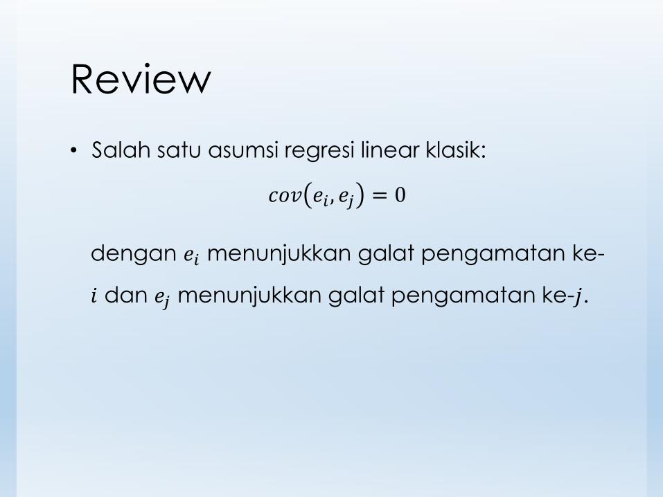
• Salah satu asumsi regresi linear klasik:
𝑐𝑜𝑣 𝑒𝑖 , 𝑒𝑗 = 0
dengan 𝑒𝑖 menunjukkan galat pengamatan ke-
𝑖 dan 𝑒𝑗 menunjukkan galat pengamatan ke-𝑗.
Sebab Umum TerjadinyaAutokorelasi pada Galat
• Terdapat peubah yang tidak disertakan dalammodel
• Mispesifikasi model
• Measurement error
Konsekuensi Pelanggaran AsumsiKebebasan Sisaan
• Jika asumsi tidak terpenuhi:
– Penduga masih bersifat tak bias dan konsisten
– Jika ukuran contoh besar, masih bisa diasumsikannormal
– Namun, penduga menjadi tidak efisien (bukanpenduga tak bias terbaik (BLUE)).
– Penduga galat baku menjadi tidak reliable, sehinggahasil uji-T dan F dapat menjadi tidak valid.

Deteksi Autokorelasi
• Pendekatan grafik
• Uji Durbin-Watson
• Uji Breusch-Godfrey (BG)
• …
Deteksi Autokorelasi dengan Grafik
• Plot sisaan yang diurutkan berdasarkan waktu
• Plot membentuk pola tertentu indikasiadanya autokorelasi pada sisaan
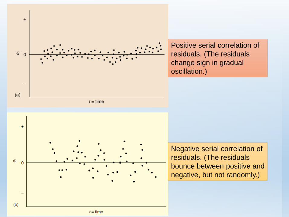
Positive serial correlation of
residuals. (The residuals
change sign in gradual
oscillation.)
Negative serial correlation of
residuals. (The residuals
bounce between positive and
negative, but not randomly.)
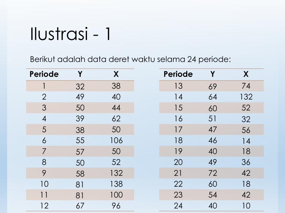
Ilustrasi - 1
Berikut adalah data deret waktu selama 24 periode:
Periode Y X Periode Y X
1 32 38 13 69 74
2 49 40 14 64 132
3 50 44 15 60 52
4 39 62 16 51 32
5 38 50 17 47 56
6 55 106 18 46 14
7 57 50 19 40 18
8 50 52 20 49 36
9 58 132 21 72 42
10 81 138 22 60 18
11 81 100 23 54 42
12 67 96 24 40 10
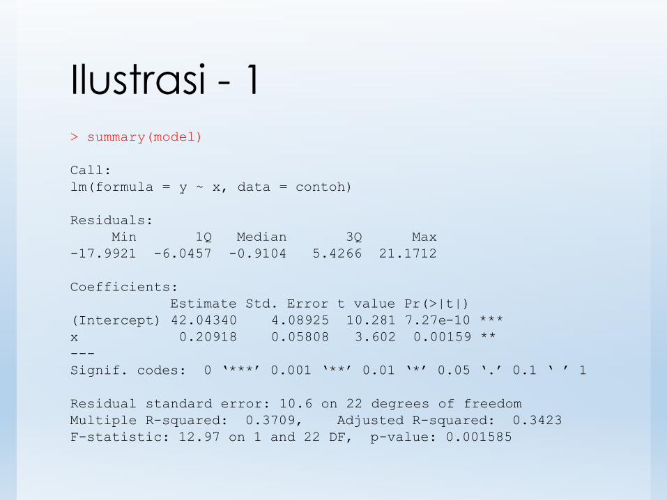
Ilustrasi - 1> summary(model)
Call:
lm(formula = y ~ x, data = contoh)
Residuals:
Min 1Q Median 3Q Max
-17.9921 -6.0457 -0.9104 5.4266 21.1712
Coefficients:
Estimate Std. Error t value Pr(>|t|)
(Intercept) 42.04340 4.08925 10.281 7.27e-10 ***
x 0.20918 0.05808 3.602 0.00159 **
---
Signif. codes: 0 ‘***’ 0.001 ‘**’ 0.01 ‘*’ 0.05 ‘.’ 0.1 ‘ ’ 1
Residual standard error: 10.6 on 22 degrees of freedom
Multiple R-squared: 0.3709, Adjusted R-squared: 0.3423
F-statistic: 12.97 on 1 and 22 DF, p-value: 0.001585
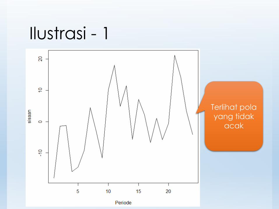
Ilustrasi - 1
Terlihat pola
yang tidak
acak

Uji Durbin-Watson
Uji Durbin Watson
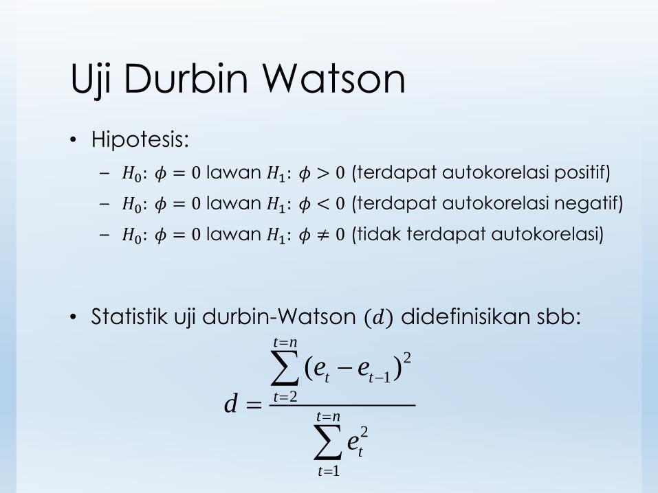
• Hipotesis:
– 𝐻0: 𝜙 = 0 lawan 𝐻1: 𝜙 > 0 (terdapat autokorelasi positif)
– 𝐻0: 𝜙 = 0 lawan 𝐻1: 𝜙 < 0 (terdapat autokorelasi negatif)
– 𝐻0: 𝜙 = 0 lawan 𝐻1: 𝜙 ≠ 0 (tidak terdapat autokorelasi)
• Statistik uji durbin-Watson (𝑑) didefinisikan sbb:
2
1
2
2
1
( )t n
t t
t
t n
t
t
e e
d
e
Asumsi pada Uji Durbin-Watson
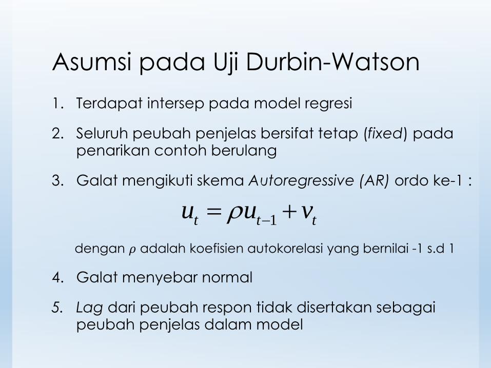
1. Terdapat intersep pada model regresi
2. Seluruh peubah penjelas bersifat tetap (fixed) padapenarikan contoh berulang
3. Galat mengikuti skema Autoregressive (AR) ordo ke-1 :
dengan 𝜌 adalah koefisien autokorelasi yang bernilai -1 s.d 1
4. Galat menyebar normal
5. Lag dari peubah respon tidak disertakan sebagaipeubah penjelas dalam model
1t t tu u v
Uji Durbin-Watson
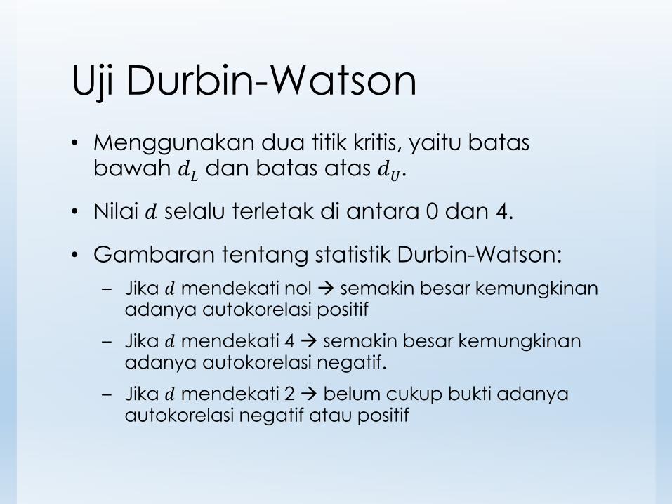
• Menggunakan dua titik kritis, yaitu batasbawah 𝑑𝐿 dan batas atas 𝑑𝑈.
• Nilai 𝑑 selalu terletak di antara 0 dan 4.
• Gambaran tentang statistik Durbin-Watson:
– Jika 𝑑 mendekati nol semakin besar kemungkinanadanya autokorelasi positif
– Jika 𝑑 mendekati 4 semakin besar kemungkinanadanya autokorelasi negatif.
– Jika 𝑑 mendekati 2 belum cukup bukti adanyaautokorelasi negatif atau positif
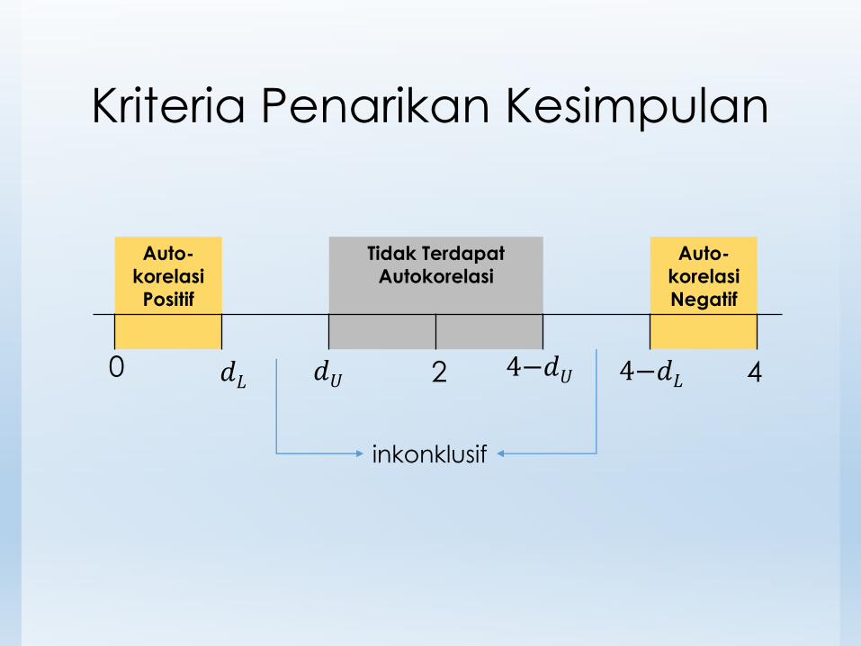
Kriteria Penarikan Kesimpulan
Auto-
korelasi
Positif
Tidak Terdapat
Autokorelasi
Auto-
korelasi
Negatif
0 𝑑𝐿 𝑑𝑈 2 4−𝑑𝑈 4−𝑑𝐿 4
inkonklusif
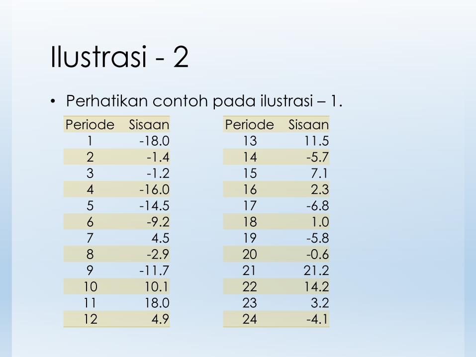
Ilustrasi - 2
• Perhatikan contoh pada ilustrasi – 1.
Periode Sisaan Periode Sisaan
1 -18.0 13 11.5
2 -1.4 14 -5.7
3 -1.2 15 7.1
4 -16.0 16 2.3
5 -14.5 17 -6.8
6 -9.2 18 1.0
7 4.5 19 -5.8
8 -2.9 20 -0.6
9 -11.7 21 21.2
10 10.1 22 14.2
11 18.0 23 3.2
12 4.9 24 -4.1

Ilustrasi - 2
𝑑 = 𝑡=2𝑡=𝑛 𝑒𝑡 − 𝑒𝑡−1
2
𝑡=1𝑡=𝑛 𝑒𝑡
2
=𝑒2 − 𝑒1
2 + 𝑒3 − 𝑒22 +⋯+ 𝑒24 − 𝑒23
2
𝑒12 + 𝑒2
2 +⋯+ 𝑒242
=−1.4 − (−18) 2 + −1.2 − (−1.4) 2 +⋯+ −4.1 − 3.2 2
(−18)2+(−1.4)2+⋯+ (−4.1)2
= 1.208767

𝑑𝐿=1.273 dan 𝑑𝑈=1.446
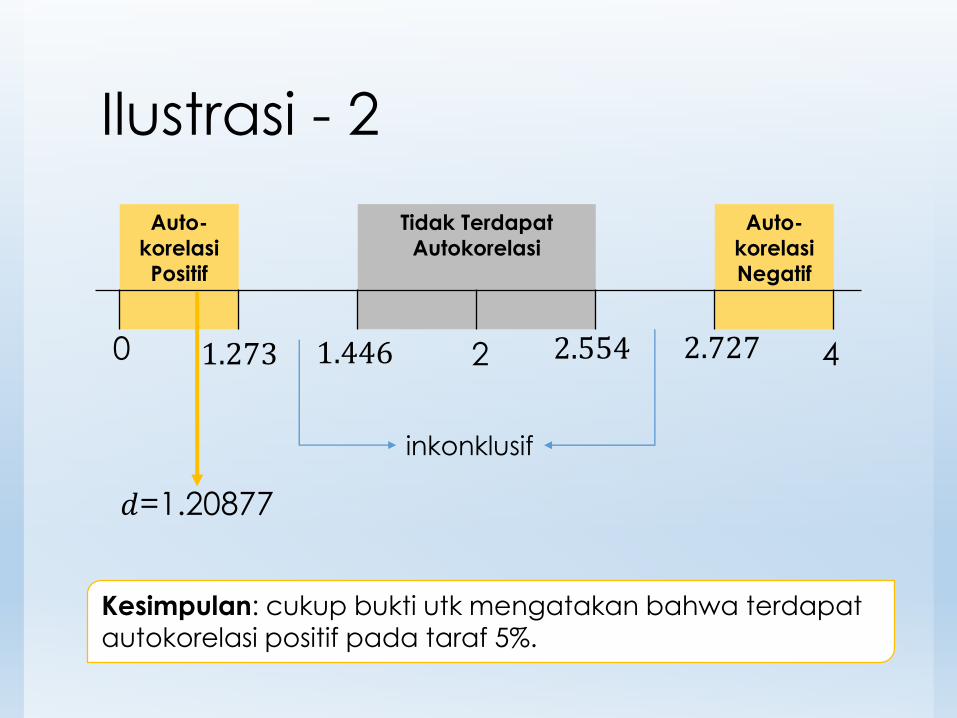
Ilustrasi - 2
Auto-
korelasi
Positif
Tidak Terdapat
Autokorelasi
Auto-
korelasi
Negatif
0 1.273 1.446 2 2.554 2.727 4
inkonklusif
𝑑=1.20877
Kesimpulan: cukup bukti utk mengatakan bahwa terdapat
autokorelasi positif pada taraf 5%.
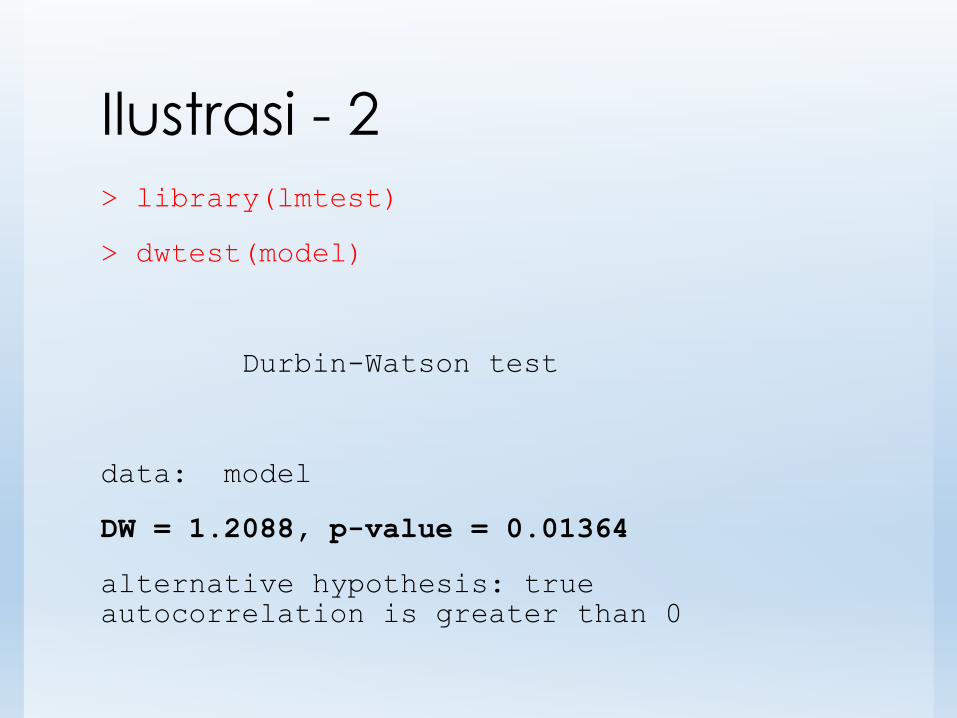
Ilustrasi - 2
> library(lmtest)
> dwtest(model)
Durbin-Watson test
data: model
DW = 1.2088, p-value = 0.01364
alternative hypothesis: true
autocorrelation is greater than 0

Uji Breuch-Godfrey
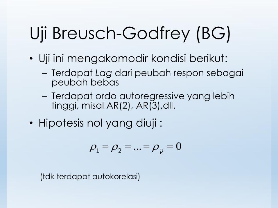
Uji Breusch-Godfrey (BG)
• Uji ini mengakomodir kondisi berikut:
– Terdapat Lag dari peubah respon sebagaipeubah bebas
– Terdapat ordo autoregressive yang lebihtinggi, misal AR(2), AR(3),dll.
• Hipotesis nol yang diuji :
(tdk terdapat autokorelasi)
1 2 ... 0p
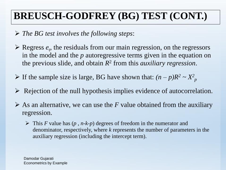
BREUSCH-GODFREY (BG) TEST (CONT.)
The BG test involves the following steps:
Regress et, the residuals from our main regression, on the regressors
in the model and the p autoregressive terms given in the equation on
the previous slide, and obtain R2 from this auxiliary regression.
If the sample size is large, BG have shown that: (n – p)R2 ~ X2p
Rejection of the null hypothesis implies evidence of autocorrelation.
As an alternative, we can use the F value obtained from the auxiliary
regression.
This F value has (p , n-k-p) degrees of freedom in the numerator and
denominator, respectively, where k represents the number of parameters in the
auxiliary regression (including the intercept term).
Damodar Gujarati
Econometrics by Example
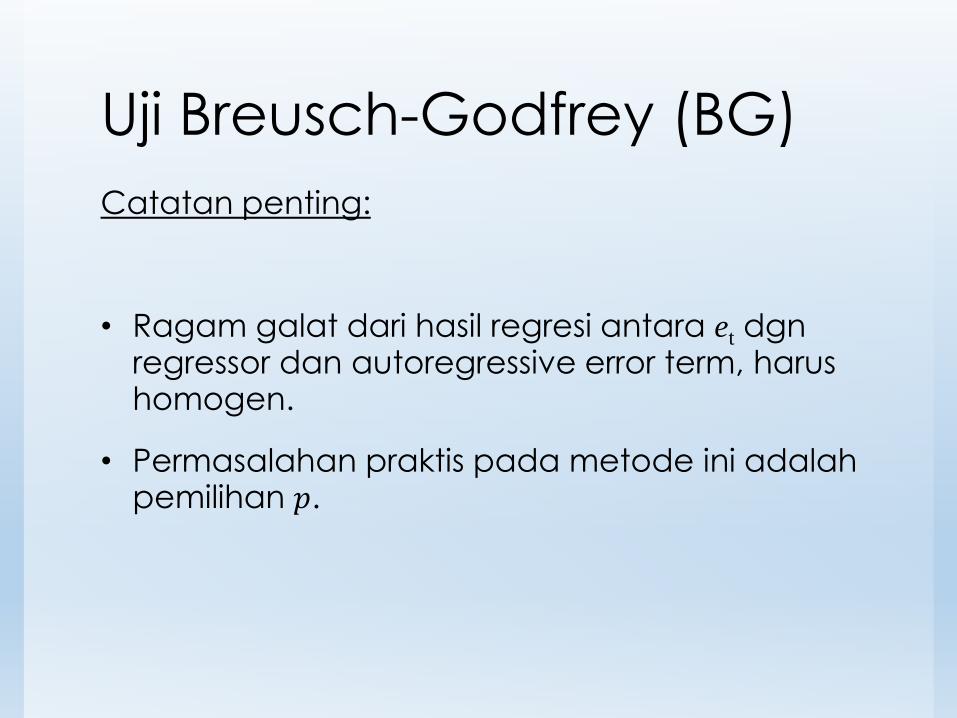
Uji Breusch-Godfrey (BG)
Catatan penting:
• Ragam galat dari hasil regresi antara et dgnregressor dan autoregressive error term, harushomogen.
• Permasalahan praktis pada metode ini adalahpemilihan 𝑝.
Pendekatan lainnya
• Runs test
• Langrange Multiplier (LM) test
• …
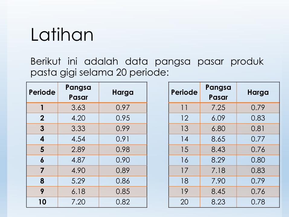
Latihan
Berikut ini adalah data pangsa pasar produkpasta gigi selama 20 periode:
PeriodePangsa
PasarHarga Periode
Pangsa
PasarHarga
1 3.63 0.97 11 7.25 0.79
2 4.20 0.95 12 6.09 0.83
3 3.33 0.99 13 6.80 0.81
4 4.54 0.91 14 8.65 0.77
5 2.89 0.98 15 8.43 0.76
6 4.87 0.90 16 8.29 0.80
7 4.90 0.89 17 7.18 0.83
8 5.29 0.86 18 7.90 0.79
9 6.18 0.85 19 8.45 0.76
10 7.20 0.82 20 8.23 0.78
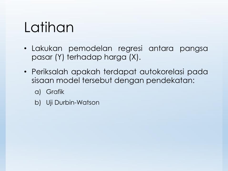
Latihan
• Lakukan pemodelan regresi antara pangsapasar (Y) terhadap harga (X).
• Periksalah apakah terdapat autokorelasi padasisaan model tersebut dengan pendekatan:
a) Grafik
b) Uji Durbin-Watson
Referensi
• Gujarati, D., McMillan, P. 2011. Econometrics by Example.
• Paulson, D.S. 2007. Handbook of Regression and Modeling: Applications for the Clinical and Pharmaceutical Industries. Boca Raton: Chapman & Hall.
• Pustaka lain yang relevan