Beberapa FungsiPeluang Kontinu (2)Pengantar Hitung Peluang - Pertemuan 10r.rahma.anisa@gmail.com

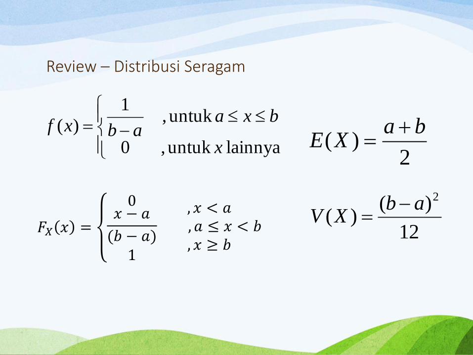
Review – Distribusi Seragam

lainnya untuk ,0

untuk ,1

)(

x

bxaabxf

𝐹𝑋 𝑥 =

0𝑥 − 𝑎

(𝑏 − 𝑎)1

, 𝑥 < 𝑎, 𝑎 ≤ 𝑥 < 𝑏, 𝑥 ≥ 𝑏

2)(

baXE

12

)()(

2abXV

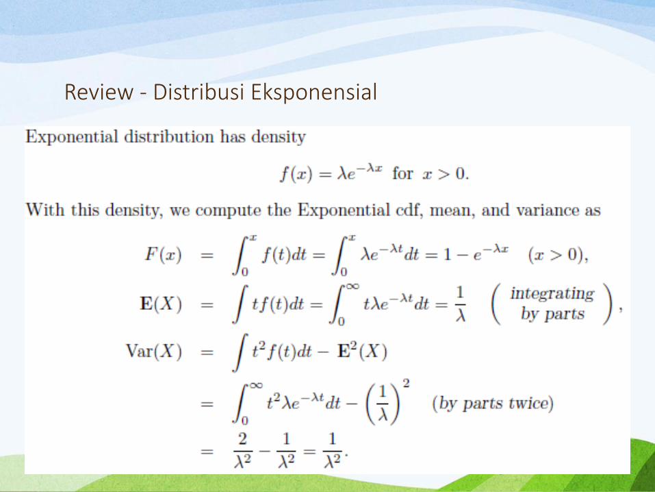
Review - Distribusi Eksponensial

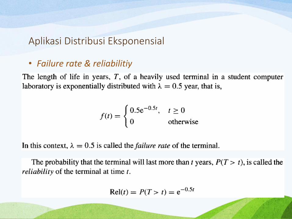
Aplikasi Distribusi Eksponensial

• Failure rate & reliabilitiy

Aplikasi Distribusi Eksponensial

• Failure rate & reliabilitiy

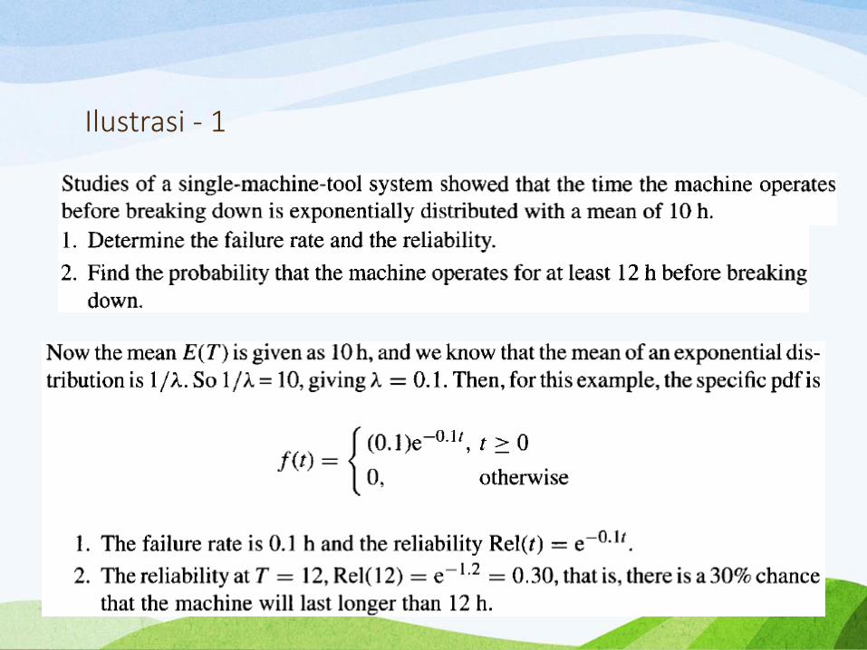
Ilustrasi - 1

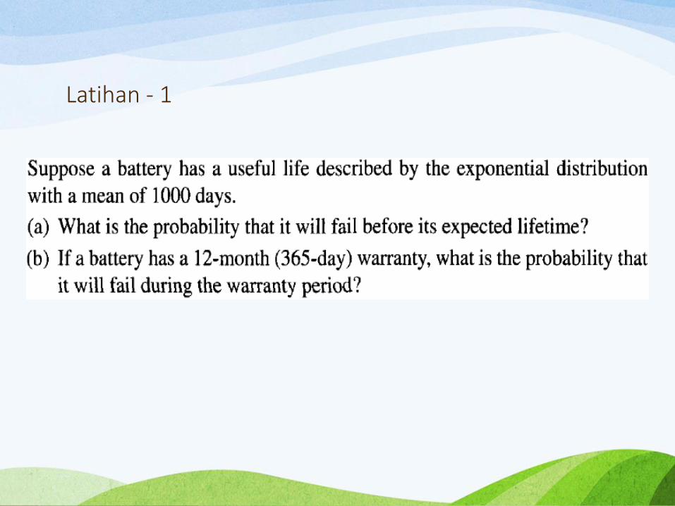
Latihan - 1

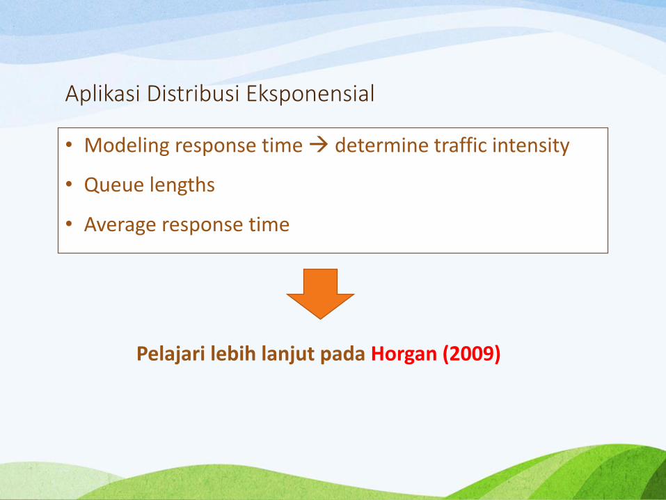
Aplikasi Distribusi Eksponensial

• Modeling response time determine traffic intensity

• Queue lengths

• Average response time

Pelajari lebih lanjut pada Horgan (2009)

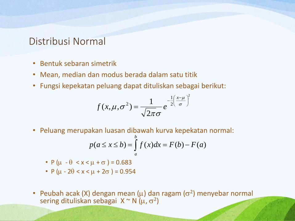
Distribusi Normal

• Bentuk sebaran simetrik

• Mean, median dan modus berada dalam satu titik

• Fungsi kepekatan peluang dapat dituliskan sebagai berikut:

• Peluang merupakan luasan dibawah kurva kepekatan normal:

• P ( - < x < + ) = 0.683

• P ( - 2 < x < + 2 ) = 0.954

• Peubah acak (X) dengan mean () dan ragam (2) menyebar normal sering dituliskan sebagai X ~ N (, 2)

2

2

1

2

2

1),,(

x

exf

b

a

aFbFdxxfbxap )()()()(

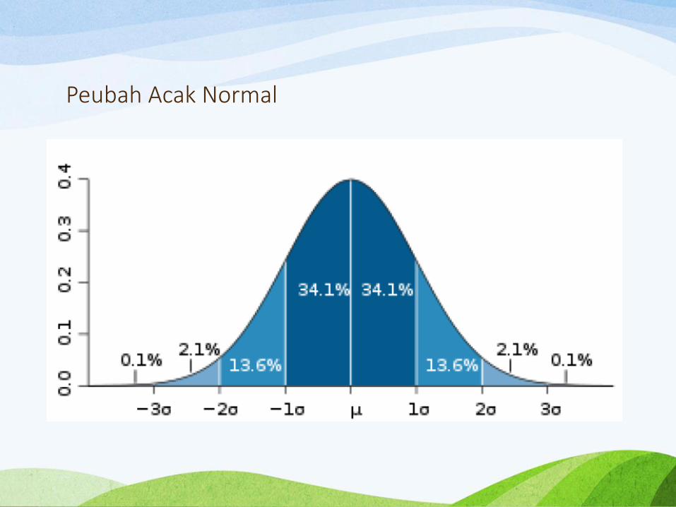
Peubah Acak Normal

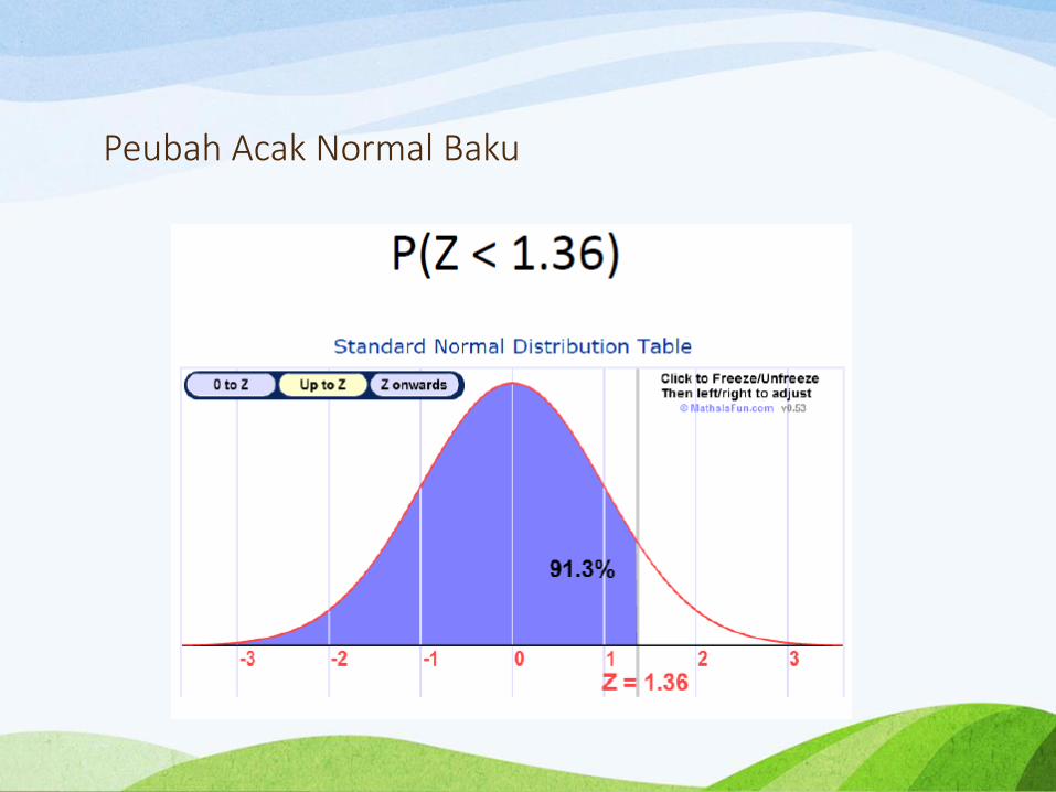
Peubah Acak Normal Baku

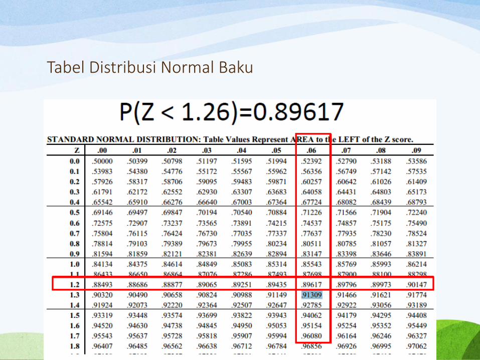
Tabel Distribusi Normal Baku

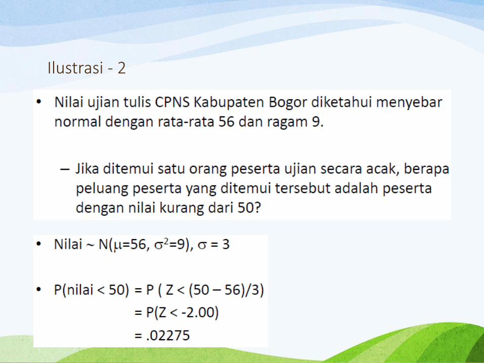
Ilustrasi - 2

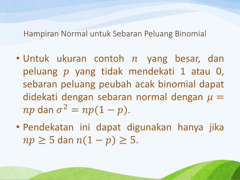
Hampiran Normal untuk Sebaran Peluang Binomial

• Untuk ukuran contoh 𝑛 yang besar, danpeluang 𝑝 yang tidak mendekati 1 atau 0,sebaran peluang peubah acak binomial dapatdidekati dengan sebaran normal dengan 𝜇 =𝑛𝑝 dan 𝜎2 = 𝑛𝑝(1 − 𝑝).

• Pendekatan ini dapat digunakan hanya jika𝑛𝑝 ≥ 5 dan 𝑛(1 − 𝑝) ≥ 5.

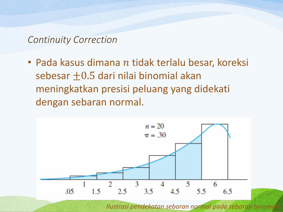
Continuity Correction

• Pada kasus dimana 𝑛 tidak terlalu besar, koreksisebesar ±0.5 dari nilai binomial akanmeningkatkan presisi peluang yang didekatidengan sebaran normal.

Ilustrasi pendekatan sebaran normal pada sebaran binomial

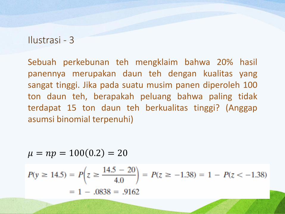
Ilustrasi - 3

Sebuah perkebunan teh mengklaim bahwa 20% hasilpanennya merupakan daun teh dengan kualitas yangsangat tinggi. Jika pada suatu musim panen diperoleh 100ton daun teh, berapakah peluang bahwa paling tidakterdapat 15 ton daun teh berkualitas tinggi? (Anggapasumsi binomial terpenuhi)

𝜇 = 𝑛𝑝 = 100 0.2 = 20

𝜎2 = 𝑛𝑝 1 − 𝑝 = 100 0.2 0.8 = 16 𝜎 = 16 = 4

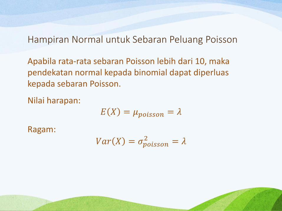
Hampiran Normal untuk Sebaran Peluang Poisson

Apabila rata-rata sebaran Poisson lebih dari 10, makapendekatan normal kepada binomial dapat diperluaskepada sebaran Poisson.

Nilai harapan:𝐸 𝑋 = 𝜇𝑝𝑜𝑖𝑠𝑠𝑜𝑛 = 𝜆

Ragam:

𝑉𝑎𝑟 𝑋 = 𝜎𝑝𝑜𝑖𝑠𝑠𝑜𝑛2 = 𝜆

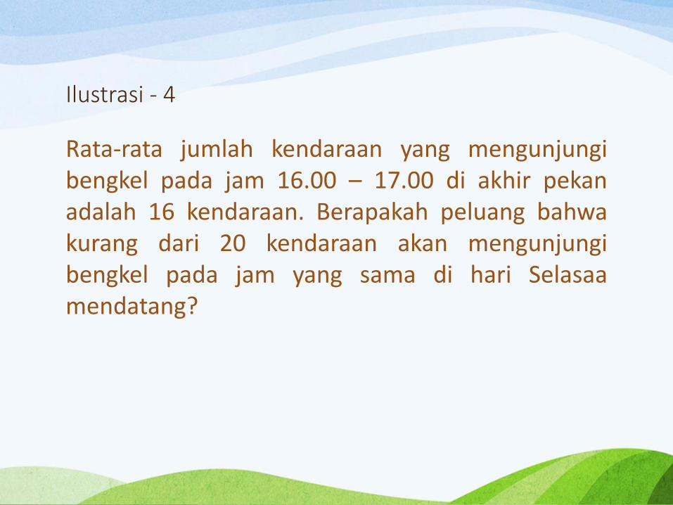
Ilustrasi - 4

Rata-rata jumlah kendaraan yang mengunjungibengkel pada jam 16.00 – 17.00 di akhir pekanadalah 16 kendaraan. Berapakah peluang bahwakurang dari 20 kendaraan akan mengunjungibengkel pada jam yang sama di hari Selasaamendatang?

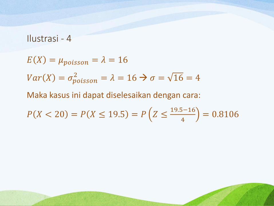
Ilustrasi - 4

𝐸 𝑋 = 𝜇𝑝𝑜𝑖𝑠𝑠𝑜𝑛 = 𝜆 = 16

𝑉𝑎𝑟 𝑋 = 𝜎𝑝𝑜𝑖𝑠𝑠𝑜𝑛2 = 𝜆 = 16 𝜎 = 16 = 4

Maka kasus ini dapat diselesaikan dengan cara:

𝑃 𝑋 < 20 = 𝑃 𝑋 ≤ 19.5 = 𝑃 𝑍 ≤19.5−16

4= 0.8106

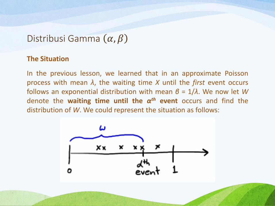
Distribusi Gamma 𝛼, 𝛽

The Situation

In the previous lesson, we learned that in an approximate Poissonprocess with mean λ, the waiting time X until the first event occursfollows an exponential distribution with mean β = 1/λ. We now let Wdenote the waiting time until the αth event occurs and find thedistribution of W. We could represent the situation as follows:

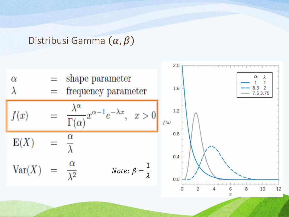
Distribusi Gamma 𝛼, 𝛽

𝛼

𝑁𝑜𝑡𝑒: 𝛽 =1

𝜆

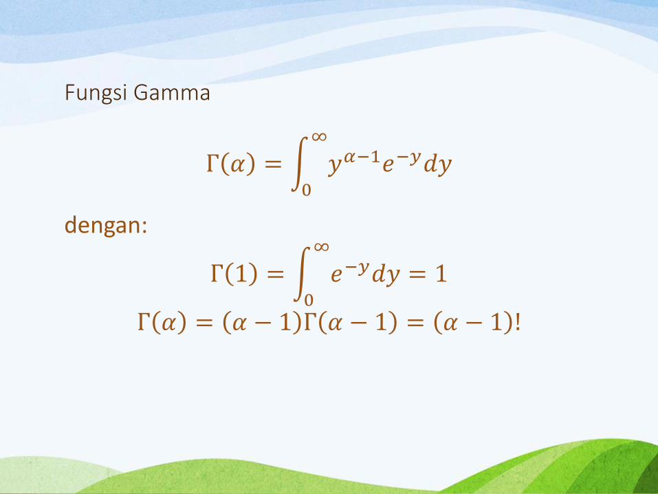
Fungsi Gamma

Γ 𝛼 = 0

∞

𝑦𝛼−1𝑒−𝑦𝑑𝑦

dengan:

Γ 1 = 0

∞

𝑒−𝑦𝑑𝑦 = 1

Γ 𝛼 = 𝛼 − 1 Γ 𝛼 − 1 = 𝛼 − 1 !

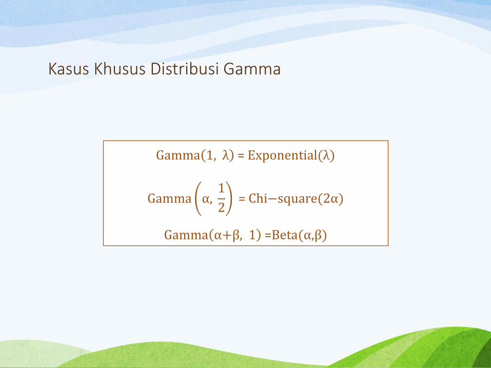
Kasus Khusus Distribusi Gamma

Gamma 1, λ = Exponential(λ)

Gamma α,1

2= Chi−square(2α)

Gamma α+β, 1 =Beta(α,β)

Ilustrasi - 4

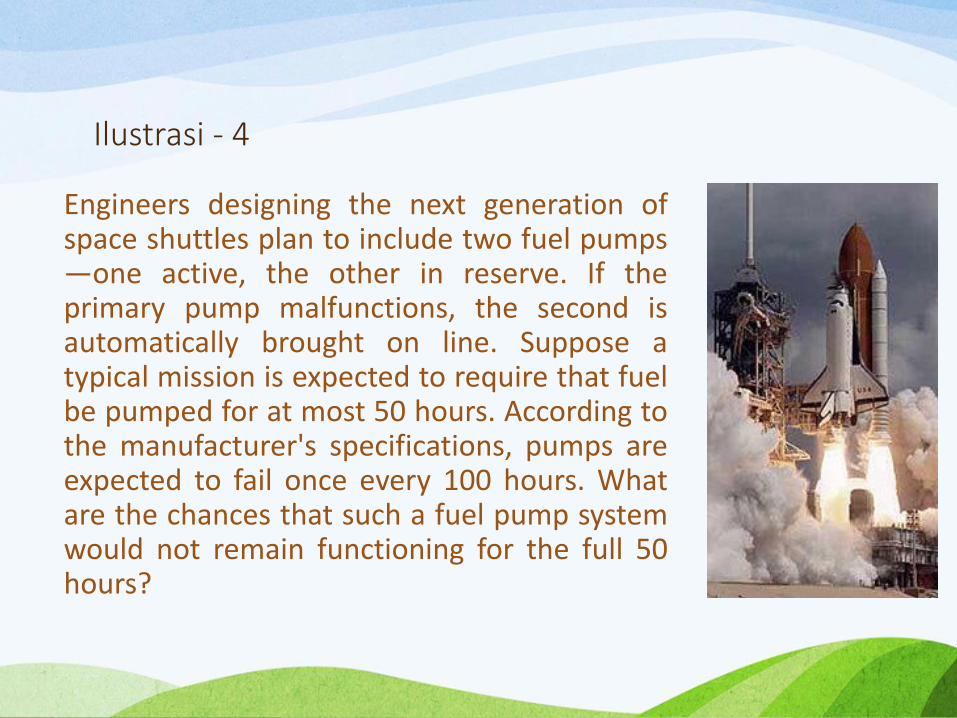
Engineers designing the next generation ofspace shuttles plan to include two fuel pumps—one active, the other in reserve. If theprimary pump malfunctions, the second isautomatically brought on line. Suppose atypical mission is expected to require that fuelbe pumped for at most 50 hours. According tothe manufacturer's specifications, pumps areexpected to fail once every 100 hours. Whatare the chances that such a fuel pump systemwould not remain functioning for the full 50hours?

Ilustrasi - 4

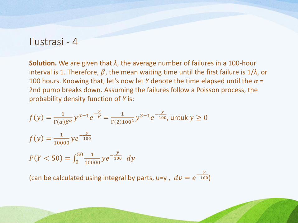
Solution. We are given that λ, the average number of failures in a 100-hour interval is 1. Therefore, 𝛽, the mean waiting time until the first failure is 1/λ, or 100 hours. Knowing that, let's now let Y denote the time elapsed until the α = 2nd pump breaks down. Assuming the failures follow a Poisson process, the probability density function of Y is:

𝑓 𝑦 =1

Γ 𝛼 𝛽𝛼𝑦𝛼−1𝑒

−𝑦

𝛽 =1

Γ 2 1002𝑦2−1𝑒−

𝑦

100, untuk 𝑦 ≥ 0

𝑓 𝑦 =1

10000𝑦𝑒−

𝑦

100

𝑃 𝑌 < 50 = 050 1

10000𝑦𝑒−

𝑦

100 𝑑𝑦

(can be calculated using integral by parts, u=y , 𝑑𝑣 = 𝑒−𝑦

100)

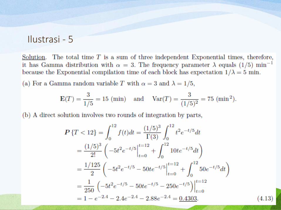
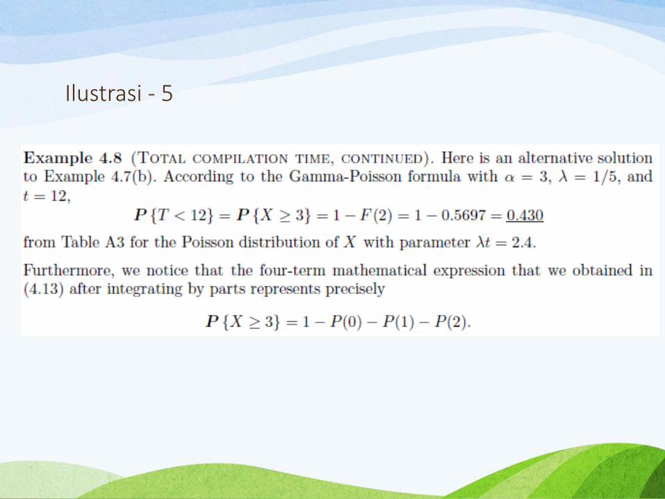
Ilustrasi – 5

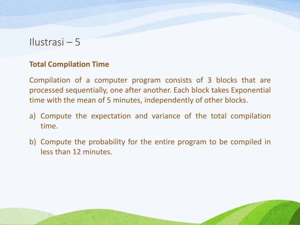
Total Compilation Time

Compilation of a computer program consists of 3 blocks that areprocessed sequentially, one after another. Each block takes Exponentialtime with the mean of 5 minutes, independently of other blocks.

a) Compute the expectation and variance of the total compilationtime.

b) Compute the probability for the entire program to be compiled inless than 12 minutes.

Ilustrasi - 5

Ilustrasi - 5

Latihan - 2

Lifetimes of computer memory chips have Gammadistribution with expectation μ = 12 years andstandard deviation σ = 4 years. What is theprobability that such a chip has a lifetime between8 and 10 years?

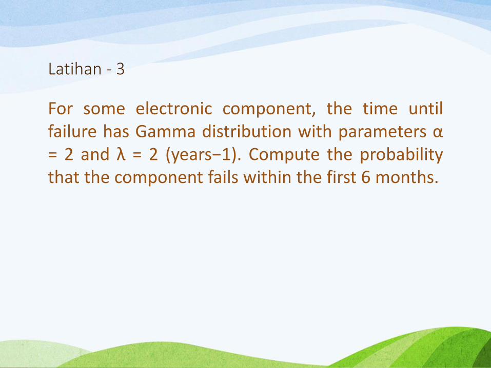
Latihan - 3

For some electronic component, the time untilfailure has Gamma distribution with parameters α= 2 and λ = 2 (years−1). Compute the probabilitythat the component fails within the first 6 months.

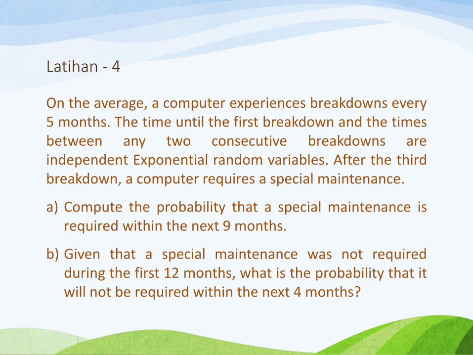
Latihan - 4

On the average, a computer experiences breakdowns every5 months. The time until the first breakdown and the timesbetween any two consecutive breakdowns areindependent Exponential random variables. After the thirdbreakdown, a computer requires a special maintenance.

a) Compute the probability that a special maintenance isrequired within the next 9 months.

b) Given that a special maintenance was not requiredduring the first 12 months, what is the probability that itwill not be required within the next 4 months?

Referensi

1. Baron, M. 2014. Probability and Statistics for Computer Scientist, Second Edition.Boca Raton: CRC Press Taylor & Francis Group.

2. [Department of Statistics Online Programs]. 2016. A Gamma Example. ThePennsylvania State University.https://onlinecourses.science.psu.edu/stat414/node/144 [27 November 2016]

3. Horgan, J.M. 2009. Probability with R: An Introduction with Computer ScienceApplications. New Jersey: John Wiley & Sons.

4. Montgomery, D.C, Runger, G.C. 2003. Applied Statistics and Probability forEngineers, Third Edition. New Jersey: John Wiley & Sons.

5. Referensi lain yang relevan.