nama kursus : rekabentuk dan analisis eksperimen...
TRANSCRIPT

1
i
NAMA KURSUS : REKABENTUK DAN ANALISIS EKSPERIMEN (Experimental Design and Analysis) KOD KURSUS : PRT 3202 KREDIT : 3 (2+1) JUMLAH JAM PEMBELAJARAN PELAJAR : 120 jam per semester PRASYARAT : Tiada HASIL PEMBELAJARAN : Pelajar dapat:
1. merumuskan kesimpulan daripada eksperimen (C5, LL) 2. mengorganisasikan eksperimen berasaskan objektif dan
keadaan persekitaran (P4, CTPS) 3. memilih kaedah sesuai untuk analisis data (A3)
SINOPSIS : Kursus ini meliputi kaedah melaksanakan eksperimen yang merangkumi rekabentuk eksperimen, persampelan, analisis dan intepretasi data, dan membuat rumusan. (This course covers the methods of conducting experiments including experimental design, sampling, data analysis and interpretation, and formulating conclusions.)
KANDUNGAN
Jam Pembelajaran
Bersemuka
KULIAH : 1. 2.
Prinsip asas - jenis-jenis eksperimen - pemilihan tapak eksperimen - keseragaman kawasan - langkah-langkah dalam melaksana
eksperimen - jenis data untuk dikumpulkan - ujian hipotesis Petak ekperimen lapangan - kawalan ralat eksperimen - saiz petak - keseragaman petak - kesan sempadan petak
3
3

2
ii
3. Reka bentuk eksperimen asas 4 - kepentingan merawak
- reka bentuk rawak lengkap (CRD) - konsep replikasi dan blok - reka bentuk rawak blok lengkap
(RCBD)
4.
Analisis varians (ANOVA) - andaian untuk memenuhi syarat
ANOVA - penjelmaan data - ANOVA untuk CRD dan RCBD
4
5. Perbandingan min rawatan - perbandingan min antara rawatan - regresi dalam ANOVA
3
6. Analisis untuk variabel tak normal - analisis untuk bilangan - kaedah Non-Parametrik
3
7. Eksperimen faktoran - kesan utama dan interaksi - kontras berortogon
4
8. Eksperimen dengan saiz petak berbeza - reka bentuk petak belahan (Split
Plot) - reka bentuk petak jaluran (Strip Pot) - pengukuran berulang
4
Jumlah 28
Jam Pembelajaran
Bersemuka
AMALI : 1. Menggunakan perisian lembaran untuk menangani data
6
2. Menggunakan perisian statistik untuk
meganalisis data 6
iii
3. Melaksanakan ANOVA sehala (CRD) 3 4. Melaksanakan ANOVA dua hala
(RCBD) 3
5. Melaksanakan perbandingan antara
rawatan 3
6. Melaksanakan penjelmaan data 3 7. Melaksanakan kaedah non-parametrik 6 8. Menganalisis eksperimen faktoran 6 9. Melaksanakan kontras berortogon 3 10. Melaksanakan ANOVA untuk reka
bentuk petak belahan 3
Jumlah 42
PENILAIAN : Kerja Kursus 60 % Peperiksaan Akhir 40 % RUJUKAN : 1.
2.
Casella, G. (2008). Statistical Design. New York: Springer Clewer, A.G. & Scarisbrick, D. H.. (2001). Practical Statistics and Experimental Design for Plant and Crop Science. New York: John Wiley & Sons.
3. Gomez, K.A. & Gomez, A.G. (2005). Statistical Procedures for Agricultural Research (4th Edition). New York: John Wiley & Sons.
4. Hinkelmann, K. & Kempthorne, O. (2007). Design and Analysis of Experiments, Introduction to Experimental Design (2nd Edition). New York: Wiley-Interscience.
5. Petersen, R. G. (1994). Agricultural Field Experiments: Design and Analysis. New York: Marcel Dekker.

3
ii
3. Reka bentuk eksperimen asas 4 - kepentingan merawak
- reka bentuk rawak lengkap (CRD) - konsep replikasi dan blok - reka bentuk rawak blok lengkap
(RCBD)
4.
Analisis varians (ANOVA) - andaian untuk memenuhi syarat
ANOVA - penjelmaan data - ANOVA untuk CRD dan RCBD
4
5. Perbandingan min rawatan - perbandingan min antara rawatan - regresi dalam ANOVA
3
6. Analisis untuk variabel tak normal - analisis untuk bilangan - kaedah Non-Parametrik
3
7. Eksperimen faktoran - kesan utama dan interaksi - kontras berortogon
4
8. Eksperimen dengan saiz petak berbeza - reka bentuk petak belahan (Split
Plot) - reka bentuk petak jaluran (Strip Pot) - pengukuran berulang
4
Jumlah 28
Jam Pembelajaran
Bersemuka
AMALI : 1. Menggunakan perisian lembaran untuk menangani data
6
2. Menggunakan perisian statistik untuk
meganalisis data 6
iii
3. Melaksanakan ANOVA sehala (CRD) 3 4. Melaksanakan ANOVA dua hala
(RCBD) 3
5. Melaksanakan perbandingan antara
rawatan 3
6. Melaksanakan penjelmaan data 3 7. Melaksanakan kaedah non-parametrik 6 8. Menganalisis eksperimen faktoran 6 9. Melaksanakan kontras berortogon 3 10. Melaksanakan ANOVA untuk reka
bentuk petak belahan 3
Jumlah 42
PENILAIAN : Kerja Kursus 60 % Peperiksaan Akhir 40 % RUJUKAN : 1.
2.
Casella, G. (2008). Statistical Design. New York: Springer Clewer, A.G. & Scarisbrick, D. H.. (2001). Practical Statistics and Experimental Design for Plant and Crop Science. New York: John Wiley & Sons.
3. Gomez, K.A. & Gomez, A.G. (2005). Statistical Procedures for Agricultural Research (4th Edition). New York: John Wiley & Sons.
4. Hinkelmann, K. & Kempthorne, O. (2007). Design and Analysis of Experiments, Introduction to Experimental Design (2nd Edition). New York: Wiley-Interscience.
5. Petersen, R. G. (1994). Agricultural Field Experiments: Design and Analysis. New York: Marcel Dekker.

4
iv
EEXXPPEERRIIMMEENNTTAALL DDEESSIIGGNN AANNDD AANNAALLYYSSIISS
PPRRTT 33220022
DR. ANUAR ABD RAHIM Department of Land Management
Faculty of Agriculture Universiti Putra Malaysia
43400 UPM Serdang Selangor Darul Ehsan
v
COURSE INTRODUCTION
a. Course Information
Department : Land Management
Course Name : EExxppeerriimmeennttaall DDeessiiggnn aanndd AAnnaallyyssiiss
CCoouurrssee CCooddee : PRT 3202
Credit Hours : 3 (2+1)
Course Description and Summary
The course consists of 2 hours lecture and 3 hours laboratory per week. To fulfill the
laboratory requirement, student need to submit individual laboratory assignment
each week that will be given through the lecturer’s Putra Learning Management
System (LMS) or email consisting of about 42 hours per semester. Four laboratory
meetings will be conducted per semester. The laboratory assignment is self-learning
due to the distance learning that permit limited meetings.

5
iv
EEXXPPEERRIIMMEENNTTAALL DDEESSIIGGNN AANNDD AANNAALLYYSSIISS
PPRRTT 33220022
DR. ANUAR ABD RAHIM Department of Land Management
Faculty of Agriculture Universiti Putra Malaysia
43400 UPM Serdang Selangor Darul Ehsan
v
COURSE INTRODUCTION
a. Course Information
Department : Land Management
Course Name : EExxppeerriimmeennttaall DDeessiiggnn aanndd AAnnaallyyssiiss
CCoouurrssee CCooddee : PRT 3202
Credit Hours : 3 (2+1)
Course Description and Summary
The course consists of 2 hours lecture and 3 hours laboratory per week. To fulfill the
laboratory requirement, student need to submit individual laboratory assignment
each week that will be given through the lecturer’s Putra Learning Management
System (LMS) or email consisting of about 42 hours per semester. Four laboratory
meetings will be conducted per semester. The laboratory assignment is self-learning
due to the distance learning that permit limited meetings.

6
vi
b. Writer Information
Name : Anuar Abd Rahim, PhD
Address : Department of Land Management,
Faculty of Agriculture, Universiti Putra Malaysia
43400 UPM Serdang Selangor
Telephone No. : 03-89474857
Fax No. : 03-89408316
e-mail : [email protected]
c. Course Objectives/ Learning Outcomes Student will be able to:
Formulate summary and conclusion from experiments (C5, LL)
1. Organize experiments based on the objectives and real situation
of the environment (P4, CTPS)
2. Select suitable methodology in analyzing data (A3)
d. Course Synopsis This course covers the methods of conducting experiments including
experimental design, data sampling and analysis, and formulating conclusions
from the analysis.
vii
e. Course Content - Principles of Experimental Design
- Experimental Designs
- Analysis of Variances
- Comparison of Treatment Means
- Data Transformation
- Non-parametric Tests
- Factorial Experiments
- Experiments with Different Size of Experimental Plots
f. Instructions for Laboratory Assignments
Laboratory assignments will be displayed each week through the lecturer’s
Putra Learning Management System (LMS) or email. These assignments have
to be completed manually and using statistical software. The reports should
be sent within one week after being introduced via email or any convenience
way to the assigned lecturer.

7
vi
b. Writer Information
Name : Anuar Abd Rahim, PhD
Address : Department of Land Management,
Faculty of Agriculture, Universiti Putra Malaysia
43400 UPM Serdang Selangor
Telephone No. : 03-89474857
Fax No. : 03-89408316
e-mail : [email protected]
c. Course Objectives/ Learning Outcomes Student will be able to:
Formulate summary and conclusion from experiments (C5, LL)
1. Organize experiments based on the objectives and real situation
of the environment (P4, CTPS)
2. Select suitable methodology in analyzing data (A3)
d. Course Synopsis This course covers the methods of conducting experiments including
experimental design, data sampling and analysis, and formulating conclusions
from the analysis.
vii
e. Course Content - Principles of Experimental Design
- Experimental Designs
- Analysis of Variances
- Comparison of Treatment Means
- Data Transformation
- Non-parametric Tests
- Factorial Experiments
- Experiments with Different Size of Experimental Plots
f. Instructions for Laboratory Assignments
Laboratory assignments will be displayed each week through the lecturer’s
Putra Learning Management System (LMS) or email. These assignments have
to be completed manually and using statistical software. The reports should
be sent within one week after being introduced via email or any convenience
way to the assigned lecturer.
8
viii
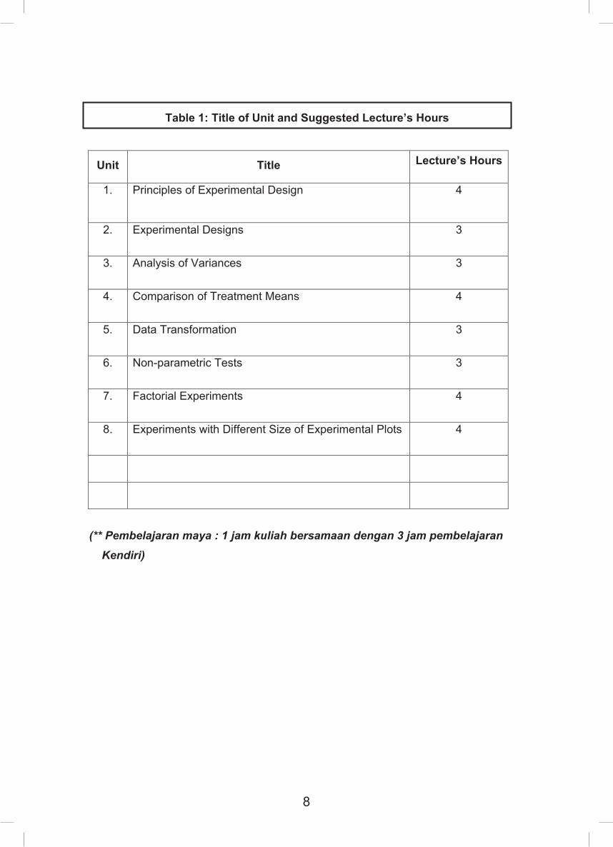
Table 1: Title of Unit and Suggested Lecture’s Hours
Unit Title Lecture’s Hours
1. Principles of Experimental Design
4
2. Experimental Designs
3
3. Analysis of Variances
3
4. Comparison of Treatment Means
4
5. Data Transformation
3
6. Non-parametric Tests
3
7. Factorial Experiments
4
8. Experiments with Different Size of Experimental Plots
4
(** Pembelajaran maya : 1 jam kuliah bersamaan dengan 3 jam pembelajaran
Kendiri)
ix
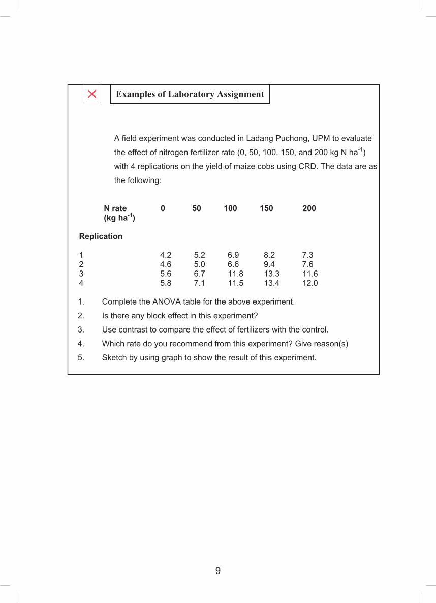
A field experiment was conducted in Ladang Puchong, UPM to evaluate
the effect of nitrogen fertilizer rate (0, 50, 100, 150, and 200 kg N ha-1)
with 4 replications on the yield of maize cobs using CRD. The data are as
the following:
N rate 0 50 100 150 200 (kg ha-1) Replication 1 4.2 5.2 6.9 8.2 7.3 2 4.6 5.0 6.6 9.4 7.6 3 5.6 6.7 11.8 13.3 11.6 4 5.8 7.1 11.5 13.4 12.0
1. Complete the ANOVA table for the above experiment.
2. Is there any block effect in this experiment?
3. Use contrast to compare the effect of fertilizers with the control.
4. Which rate do you recommend from this experiment? Give reason(s)
5. Sketch by using graph to show the result of this experiment.
Examples of Laboratory Assignment
9
viii
Table 1: Title of Unit and Suggested Lecture’s Hours
Unit Title Lecture’s Hours
1. Principles of Experimental Design
4
2. Experimental Designs
3
3. Analysis of Variances
3
4. Comparison of Treatment Means
4
5. Data Transformation
3
6. Non-parametric Tests
3
7. Factorial Experiments
4
8. Experiments with Different Size of Experimental Plots
4
(** Pembelajaran maya : 1 jam kuliah bersamaan dengan 3 jam pembelajaran
Kendiri)
ix
A field experiment was conducted in Ladang Puchong, UPM to evaluate
the effect of nitrogen fertilizer rate (0, 50, 100, 150, and 200 kg N ha-1)
with 4 replications on the yield of maize cobs using CRD. The data are as
the following:
N rate 0 50 100 150 200 (kg ha-1) Replication 1 4.2 5.2 6.9 8.2 7.3 2 4.6 5.0 6.6 9.4 7.6 3 5.6 6.7 11.8 13.3 11.6 4 5.8 7.1 11.5 13.4 12.0
1. Complete the ANOVA table for the above experiment.
2. Is there any block effect in this experiment?
3. Use contrast to compare the effect of fertilizers with the control.
4. Which rate do you recommend from this experiment? Give reason(s)
5. Sketch by using graph to show the result of this experiment.
Examples of Laboratory Assignment

10
x
g. Course Evaluation
Evaluation for this course is divided into:
(i) Coursework
Laboratory assignments (individual) 40 %
(ii) Mid-Term Examination 20%
(i) + (ii) 60% (ii) Final Examination 40%
Total 100% ** Course evaluation can be changed from time to time depending to the lecturer.
Suggested Learning Activities
1. Lecture 8 hours
2. Self Learning 45 hours per week
3. Tutorials (4 sessions) 12 hours
4. Online/Email/Telephone/LMS/Maya Class with Lecturer 10 hours
5. Laboratory Assignments 42 hours Total Hours 117 hours
xi
h. Mid-term Examination
Mid-term examination has to be taken by the student. Questions are based on
the modules that presented and in the form of subjective. This examination will
consists of units 1 to 4, and it can be adjusted in terms of form and number
of questions, topics and marks, and will be discussed during direct
meeting between the students and the lecturer concern
i. Final Examination
Questions will consist of all the units and topics that are presented in the module.
Students can consult the lecturer when concern for update details of
the examination. Questions will be asked in the form of subjective and
applications

11
x
g. Course Evaluation
Evaluation for this course is divided into:
(i) Coursework
Laboratory assignments (individual) 40 %
(ii) Mid-Term Examination 20%
(i) + (ii) 60% (ii) Final Examination 40%
Total 100% ** Course evaluation can be changed from time to time depending to the lecturer.
Suggested Learning Activities
1. Lecture 8 hours
2. Self Learning 45 hours per week
3. Tutorials (4 sessions) 12 hours
4. Online/Email/Telephone/LMS/Maya Class with Lecturer 10 hours
5. Laboratory Assignments 42 hours Total Hours 117 hours
xi
h. Mid-term Examination
Mid-term examination has to be taken by the student. Questions are based on
the modules that presented and in the form of subjective. This examination will
consists of units 1 to 4, and it can be adjusted in terms of form and number
of questions, topics and marks, and will be discussed during direct
meeting between the students and the lecturer concern
i. Final Examination
Questions will consist of all the units and topics that are presented in the module.
Students can consult the lecturer when concern for update details of
the examination. Questions will be asked in the form of subjective and
applications

12
xii
.
SECTION A Answer all questions in this section
1. Draw the arrangement of all the experimental units for the following:
(a) Source of Variation df
Block 4
Treatments 3 Error 12
Total 19 (5 marks)
(b)
Source of Variation df
Column 4
Row 4
Treatments 4
Error 12
Total 24 (5 marks)
Examples of mid-term and final examinations
:
xiii
j. Main References
1. Casella, G. (2008). Statistical Design. New York: Springer 2 Clewer, A.G. and Scarisbrick, D. H. (2001). Practical Statistics
and Experimental Design for Plant and Crop Science. New York: John Wiley and Sons.
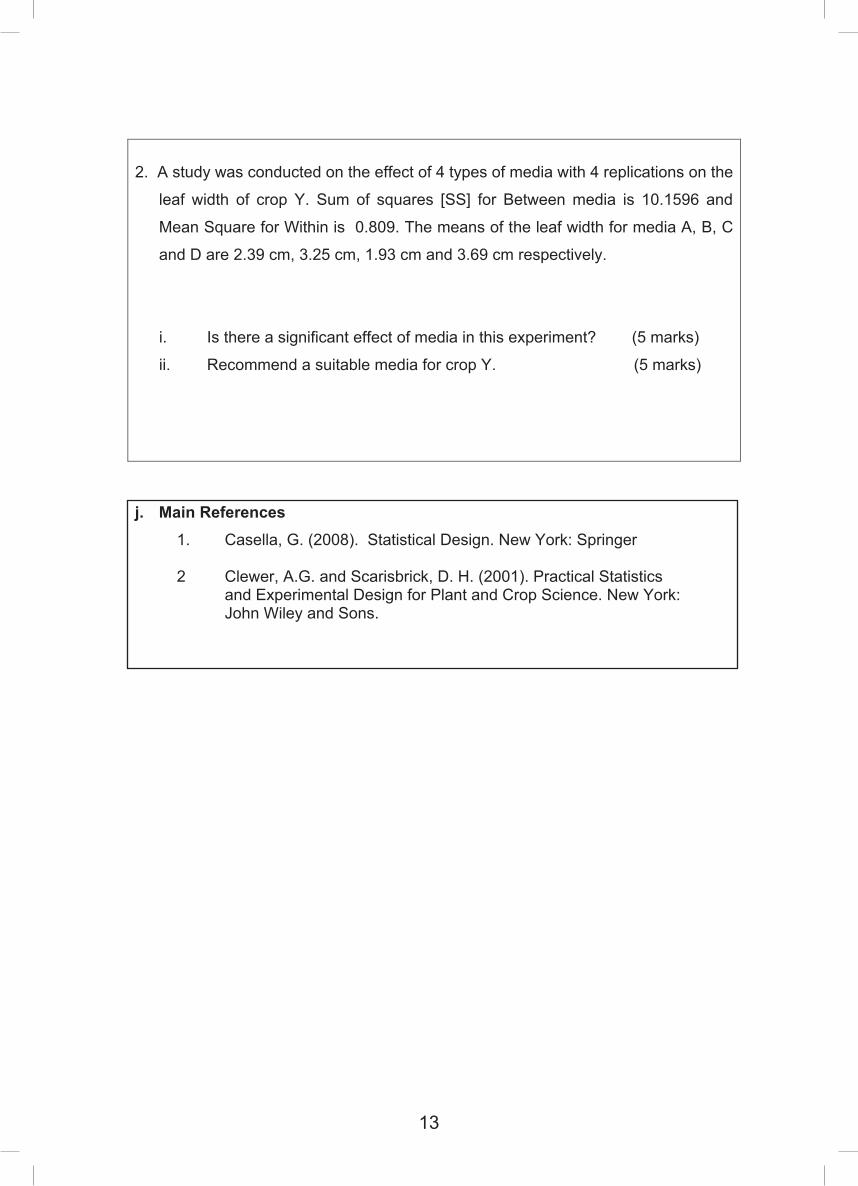
2. A study was conducted on the effect of 4 types of media with 4 replications on the
leaf width of crop Y. Sum of squares [SS] for Between media is 10.1596 and
Mean Square for Within is 0.809. The means of the leaf width for media A, B, C
and D are 2.39 cm, 3.25 cm, 1.93 cm and 3.69 cm respectively.
i. Is there a significant effect of media in this experiment? (5 marks)
ii. Recommend a suitable media for crop Y. (5 marks)
13
xii
.
SECTION A Answer all questions in this section
1. Draw the arrangement of all the experimental units for the following:
(a) Source of Variation df
Block 4
Treatments 3 Error 12
Total 19 (5 marks)
(b)
Source of Variation df
Column 4
Row 4
Treatments 4
Error 12
Total 24 (5 marks)
Examples of mid-term and final examinations
:
xiii
j. Main References
1. Casella, G. (2008). Statistical Design. New York: Springer 2 Clewer, A.G. and Scarisbrick, D. H. (2001). Practical Statistics
and Experimental Design for Plant and Crop Science. New York: John Wiley and Sons.
2. A study was conducted on the effect of 4 types of media with 4 replications on the
leaf width of crop Y. Sum of squares [SS] for Between media is 10.1596 and
Mean Square for Within is 0.809. The means of the leaf width for media A, B, C
and D are 2.39 cm, 3.25 cm, 1.93 cm and 3.69 cm respectively.
i. Is there a significant effect of media in this experiment? (5 marks)
ii. Recommend a suitable media for crop Y. (5 marks)

14
xiv
k. Extra References
1. Gomez, K. A. and Gomez, A.G. (2005). Statistical Procedures for Agricultural Research (4th Edition). New York: John Wiley and Sons. .
2. Hinkelmann, K. and Kempthorne, O. (2007). Design and Analysis
of Experiments. Introduction to Experimental Design (2nd). New York: Wiley-Interscience.
3. Peterson, R. G. (1994). Agricultural Field Experiments: Design and Analysis. New York: Marcel Dekker.
4. Adele. M. Holman (1989). Family Assessment: Tools for Understanding and Invention. New York: Sage Publication.
l. Information of icon in the module
a)
Objective Objective of module, unit or topic
b)
Introduction Introduction to unit, topic or sub-topic
c)
Important Content
Important content in unit or topic
d)
Attention
This symbol is used for information to be given attention by the students
xv
Content
Unit Title
Page
1
Principles of Experimental Design
Topic 1: Experiment
Topic 2: Treatment
Topic 3: Experimental Unit
Topic 4: Sample
Topic 5: Replication
Topic 6: Randomization
Topic 7. Variables
Topic 8: Control
Topic 9: Responses
Topic 10: Experimental Error
Topic 11: Types of Experiment
Topic 12: Selection of Test Site
Topic 13: Uniformity of Experiment Site
Topic 14: Procedure in Planning an Experiment
Topic 15: Types of Measurement /Data
Topic 16: Hypothesis Testing
Topic 17: Methods of Error Control in Experiment
Topic 18: Plot Size and Shape
Topic 19: Uniformity of Experimental Plot
1
2
3
4
5
6
7
8
8
9
10
11
12
13
13
14
15
16
16
2 Experimental Designs
Topic 1: Complete Randomized Design
Topic 2: Randomized Complete Block Design
Topic 3: Latin Square Design
18
20
22
15
xiv
k. Extra References
1. Gomez, K. A. and Gomez, A.G. (2005). Statistical Procedures for Agricultural Research (4th Edition). New York: John Wiley and Sons. .
2. Hinkelmann, K. and Kempthorne, O. (2007). Design and Analysis
of Experiments. Introduction to Experimental Design (2nd). New York: Wiley-Interscience.
3. Peterson, R. G. (1994). Agricultural Field Experiments: Design and Analysis. New York: Marcel Dekker.
4. Adele. M. Holman (1989). Family Assessment: Tools for Understanding and Invention. New York: Sage Publication.
l. Information of icon in the module
a)
Objective Objective of module, unit or topic
b)
Introduction Introduction to unit, topic or sub-topic
c)
Important Content
Important content in unit or topic
d)
Attention
This symbol is used for information to be given attention by the students
xv
Content
Unit Title
Page
1
Principles of Experimental Design
Topic 1: Experiment
Topic 2: Treatment
Topic 3: Experimental Unit
Topic 4: Sample
Topic 5: Replication
Topic 6: Randomization
Topic 7. Variables
Topic 8: Control
Topic 9: Responses
Topic 10: Experimental Error
Topic 11: Types of Experiment
Topic 12: Selection of Test Site
Topic 13: Uniformity of Experiment Site
Topic 14: Procedure in Planning an Experiment
Topic 15: Types of Measurement /Data
Topic 16: Hypothesis Testing
Topic 17: Methods of Error Control in Experiment
Topic 18: Plot Size and Shape
Topic 19: Uniformity of Experimental Plot
1
2
3
4
5
6
7
8
8
9
10
11
12
13
13
14
15
16
16
2 Experimental Designs
Topic 1: Complete Randomized Design
Topic 2: Randomized Complete Block Design
Topic 3: Latin Square Design
18
20
22
16
xvi
Unit Title
Page
3 Analysis of Variances (ANOVA) Topic 1: F Distribution
Topic 2: ANOVA for One Factor Experiment
Topic 3: ANOVA for Various Designs
24
25
26
4 Comparison of Treatment Means Topic 1: Least Significant Difference (LSD)
Topic 2: Duncan’s Multiple Range Test
Topic 3: Contrast
34
37
39
5 Data Transformation
Topic 1: Log Transformation
Topic 2: Square-Root Transformation
Topic 3: Arc-sine Transformation
43
44
45
6 Non-parametric Tests
Topic 1: One Sample Sign Test
Topic 2: Paired Data Sign Test
Topic 3: Wilcoxon-Mann-Whitney
Topic 4: Chi-square Test
46
48
49
51
7 Factorial Experiment
Topic 1: Effect of Main Factor
Topic 2: Interaction Effect
57
59
8 Experiment with Different Sizes of Experimental Units Topic 1: Split Plot Design
Topic 2: Experiment with Repeated Data
66
74
1
UNIT 1
PRINCIPLES OF EXPERIMENTAL DESIGN
Introduction
In designing an experiment, it is essential to state the objectives of the experiment as
to answer the questions, stated hypothesis to be tested and the effect to be
estimated. Experimental design is how treatments under investigation are arranged
such that their effect are revealed and are accurately measured. All designs are
characterized by experimental units classified by treatments, but in some cases they
are further classified into blocks, rows, columns main plots and so on. An
experimental design can be complex or simple.
Objective To evaluate the information in the principles of the experimental design. TOPIC 1: EXPERIMENT
Important Content Experiment is an investigation to obtain
a) new information
b) proving the result of an earlier experiment
c) it is conducted to answer question(s)
17
xvi
Unit Title
Page
3 Analysis of Variances (ANOVA) Topic 1: F Distribution
Topic 2: ANOVA for One Factor Experiment
Topic 3: ANOVA for Various Designs
24
25
26
4 Comparison of Treatment Means Topic 1: Least Significant Difference (LSD)
Topic 2: Duncan’s Multiple Range Test
Topic 3: Contrast
34
37
39
5 Data Transformation
Topic 1: Log Transformation
Topic 2: Square-Root Transformation
Topic 3: Arc-sine Transformation
43
44
45
6 Non-parametric Tests
Topic 1: One Sample Sign Test
Topic 2: Paired Data Sign Test
Topic 3: Wilcoxon-Mann-Whitney
Topic 4: Chi-square Test
46
48
49
51
7 Factorial Experiment
Topic 1: Effect of Main Factor
Topic 2: Interaction Effect
57
59
8 Experiment with Different Sizes of Experimental Units Topic 1: Split Plot Design
Topic 2: Experiment with Repeated Data
66
74
1
UNIT 1
PRINCIPLES OF EXPERIMENTAL DESIGN
Introduction
In designing an experiment, it is essential to state the objectives of the experiment as
to answer the questions, stated hypothesis to be tested and the effect to be
estimated. Experimental design is how treatments under investigation are arranged
such that their effect are revealed and are accurately measured. All designs are
characterized by experimental units classified by treatments, but in some cases they
are further classified into blocks, rows, columns main plots and so on. An
experimental design can be complex or simple.
Objective To evaluate the information in the principles of the experimental design. TOPIC 1: EXPERIMENT
Important Content Experiment is an investigation to obtain
a) new information
b) proving the result of an earlier experiment
c) it is conducted to answer question(s)

18
PRT 3202 Experimental Design and Analysis PJJ UPM / UPMET
2
Laboratory Exercise
Laboratory exercise for topic 1 unit 1 will be delivered during week 1 through
Putra Learning Management System (LMS) or email.
TOPIC 2: TREATMENT
Important Content Procedure whose effect of a material to be tested and compared with other
treatments
Example 1: types of fertilizer: NPK Blue and NPK yellow
Example 2: fertilizer rates: 10, 20 and 30 kg N ha-1
Laboratory Exercise
Laboratory exercise for topic 2 unit 1 will be delivered during week 1 through
LMS or email.
PRT 3202 Experimental Design and Analysis PJJ UPM / UPMET
3
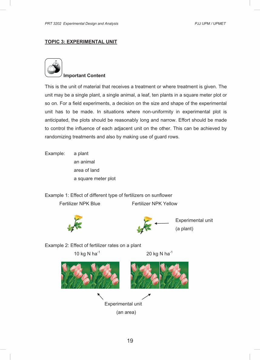
TOPIC 3: EXPERIMENTAL UNIT
Important Content This is the unit of material that receives a treatment or where treatment is given. The
unit may be a single plant, a single animal, a leaf, ten plants in a square meter plot or
so on. For a field experiments, a decision on the size and shape of the experimental
unit has to be made. In situations where non-uniformity in experimental plot is
anticipated, the plots should be reasonably long and narrow. Effort should be made
to control the influence of each adjacent unit on the other. This can be achieved by
randomizing treatments and also by making use of guard rows.
Example: a plant
an animal
area of land
a square meter plot
Example 1: Effect of different type of fertilizers on sunflower
Fertilizer NPK Blue Fertilizer NPK Yellow
Experimental unit
(a plant)
Example 2: Effect of fertilizer rates on a plant
10 kg N ha-1 20 kg N ha-1
Experimental unit
(an area)
19
PRT 3202 Experimental Design and Analysis PJJ UPM / UPMET
2
Laboratory Exercise
Laboratory exercise for topic 1 unit 1 will be delivered during week 1 through
Putra Learning Management System (LMS) or email.
TOPIC 2: TREATMENT
Important Content Procedure whose effect of a material to be tested and compared with other
treatments
Example 1: types of fertilizer: NPK Blue and NPK yellow
Example 2: fertilizer rates: 10, 20 and 30 kg N ha-1
Laboratory Exercise
Laboratory exercise for topic 2 unit 1 will be delivered during week 1 through
LMS or email.
PRT 3202 Experimental Design and Analysis PJJ UPM / UPMET
3
TOPIC 3: EXPERIMENTAL UNIT
Important Content This is the unit of material that receives a treatment or where treatment is given. The
unit may be a single plant, a single animal, a leaf, ten plants in a square meter plot or
so on. For a field experiments, a decision on the size and shape of the experimental
unit has to be made. In situations where non-uniformity in experimental plot is
anticipated, the plots should be reasonably long and narrow. Effort should be made
to control the influence of each adjacent unit on the other. This can be achieved by
randomizing treatments and also by making use of guard rows.
Example: a plant
an animal
area of land
a square meter plot
Example 1: Effect of different type of fertilizers on sunflower
Fertilizer NPK Blue Fertilizer NPK Yellow
Experimental unit
(a plant)
Example 2: Effect of fertilizer rates on a plant
10 kg N ha-1 20 kg N ha-1
Experimental unit
(an area)
20
PRT 3202 Experimental Design and Analysis PJJ UPM / UPMET
4
Laboratory Exercise
Laboratory exercise for topic 3 unit 1 will be delivered during week 1 through
LMS or email.
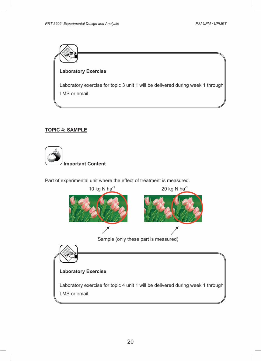
TOPIC 4: SAMPLE
Important Content Part of experimental unit where the effect of treatment is measured.
10 kg N ha-1 20 kg N ha-1
Sample (only these part is measured)
Laboratory Exercise
Laboratory exercise for topic 4 unit 1 will be delivered during week 1 through
LMS or email.
PRT 3202 Experimental Design and Analysis PJJ UPM / UPMET
5
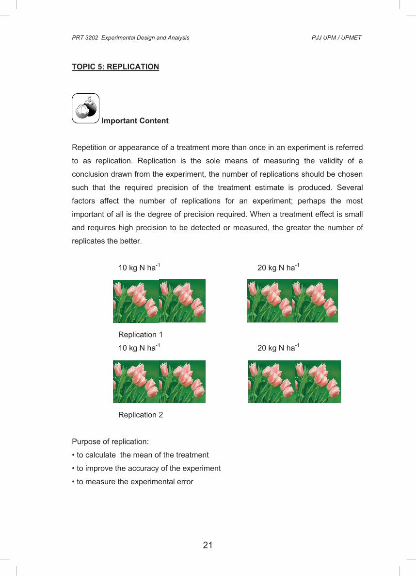
TOPIC 5: REPLICATION
Important Content Repetition or appearance of a treatment more than once in an experiment is referred
to as replication. Replication is the sole means of measuring the validity of a
conclusion drawn from the experiment, the number of replications should be chosen
such that the required precision of the treatment estimate is produced. Several
factors affect the number of replications for an experiment; perhaps the most
important of all is the degree of precision required. When a treatment effect is small
and requires high precision to be detected or measured, the greater the number of
replicates the better.
10 kg N ha-1 20 kg N ha-1
Replication 1
10 kg N ha-1 20 kg N ha-1
Replication 2
Purpose of replication:
• to calculate the mean of the treatment
• to improve the accuracy of the experiment
• to measure the experimental error
21
PRT 3202 Experimental Design and Analysis PJJ UPM / UPMET
4
Laboratory Exercise
Laboratory exercise for topic 3 unit 1 will be delivered during week 1 through
LMS or email.
TOPIC 4: SAMPLE
Important Content Part of experimental unit where the effect of treatment is measured.
10 kg N ha-1 20 kg N ha-1
Sample (only these part is measured)
Laboratory Exercise
Laboratory exercise for topic 4 unit 1 will be delivered during week 1 through
LMS or email.
PRT 3202 Experimental Design and Analysis PJJ UPM / UPMET
5
TOPIC 5: REPLICATION
Important Content Repetition or appearance of a treatment more than once in an experiment is referred
to as replication. Replication is the sole means of measuring the validity of a
conclusion drawn from the experiment, the number of replications should be chosen
such that the required precision of the treatment estimate is produced. Several
factors affect the number of replications for an experiment; perhaps the most
important of all is the degree of precision required. When a treatment effect is small
and requires high precision to be detected or measured, the greater the number of
replicates the better.
10 kg N ha-1 20 kg N ha-1
Replication 1
10 kg N ha-1 20 kg N ha-1
Replication 2
Purpose of replication:
• to calculate the mean of the treatment
• to improve the accuracy of the experiment
• to measure the experimental error
22
PRT 3202 Experimental Design and Analysis PJJ UPM / UPMET
6
Laboratory Exercise
Laboratory exercise for topic 5 unit 1 will be delivered during week 2 through
LMS or email.
TOPIC 6: RANDOMIZATION
Important Content
Arrangement of treatments of experimental unit so as that each experimental unit
has the same chance to be selected to receive a treatment
Example : Effect of 4 types of fertilizer with 2 replications.
REPLICATION 1
REPLICATION 2
Laboratory Exercise
Laboratory exercise for topic 6 unit 1 will be delivered during week 2 through
LMS or email.
A B
C D
D C
A B
PRT 3202 Experimental Design and Analysis PJJ UPM / UPMET
7
TOPIC 7: VARIABLES
Important Content Characteristics of the experimental unit that can be measured:
• Yield
• Height of a plant
• Soil pH
• Number of insects
2 types of variables
• Quantitative
• Qualitative
Laboratory Exercise
Laboratory exercise for topic 7 unit 1 will be delivered during week 2 through
LMS or email.
TOPIC 8: CONTROL
Important Content A standard treatment that is used as a baseline or basis of comparison for the other
treatments. The control treatment does not receive the treatment or the experimental
manipulation that the experimental treatments receive.

23
PRT 3202 Experimental Design and Analysis PJJ UPM / UPMET
6
Laboratory Exercise
Laboratory exercise for topic 5 unit 1 will be delivered during week 2 through
LMS or email.
TOPIC 6: RANDOMIZATION
Important Content
Arrangement of treatments of experimental unit so as that each experimental unit
has the same chance to be selected to receive a treatment
Example : Effect of 4 types of fertilizer with 2 replications.
REPLICATION 1
REPLICATION 2
Laboratory Exercise
Laboratory exercise for topic 6 unit 1 will be delivered during week 2 through
LMS or email.
A B
C D
D C
A B
PRT 3202 Experimental Design and Analysis PJJ UPM / UPMET
7
TOPIC 7: VARIABLES
Important Content Characteristics of the experimental unit that can be measured:
• Yield
• Height of a plant
• Soil pH
• Number of insects
2 types of variables
• Quantitative
• Qualitative
Laboratory Exercise
Laboratory exercise for topic 7 unit 1 will be delivered during week 2 through
LMS or email.
TOPIC 8: CONTROL
Important Content A standard treatment that is used as a baseline or basis of comparison for the other
treatments. The control treatment does not receive the treatment or the experimental
manipulation that the experimental treatments receive.

24
PRT 3202 Experimental Design and Analysis PJJ UPM / UPMET
8
Laboratory Exercise
Laboratory exercise for topic 8 unit 1 will be delivered during week 2 through
LMS or email.
TOPIC 9: RESPONSES
Important Content Outcomes that are being observed after applying a treatment to an experimental unit
Example: Treatment :- application of 3 types of nitrogen fertilizer
Response :- nitrogen content or biomass of corn plants
Laboratory Exercise
Laboratory exercise for topic 9 unit 1 will be delivered during week 2 through
LMS or email.
PRT 3202 Experimental Design and Analysis PJJ UPM / UPMET
9
TOPIC 10: EXPERIMENTAL ERROR
Important Content The random variation present in all experimental results. Errors can be minimized by
having a large sample size as well as by replications and blocking.
Laboratory Exercise
Laboratory exercise for topic 10 unit 1 will be delivered during week 2
through LMS or email.
TOPIC 11: TYPES OF EXPERIMENT
Important Content 1. Manipulative experiment – one or more conditions are varied while all other
conditions are maintained, perform under controlled conditions such as in a laboratory.
2. Field experiment – similar to manipulative experiment, but it is carried out in an open area where environmental factors and extraneous variables are present.
Laboratory Exercise
Laboratory exercise for topic 11 unit 1 will be delivered during week 3
through LMS or email.
25
PRT 3202 Experimental Design and Analysis PJJ UPM / UPMET
8
Laboratory Exercise
Laboratory exercise for topic 8 unit 1 will be delivered during week 2 through
LMS or email.
TOPIC 9: RESPONSES
Important Content Outcomes that are being observed after applying a treatment to an experimental unit
Example: Treatment :- application of 3 types of nitrogen fertilizer
Response :- nitrogen content or biomass of corn plants
Laboratory Exercise
Laboratory exercise for topic 9 unit 1 will be delivered during week 2 through
LMS or email.
PRT 3202 Experimental Design and Analysis PJJ UPM / UPMET
9
TOPIC 10: EXPERIMENTAL ERROR
Important Content The random variation present in all experimental results. Errors can be minimized by
having a large sample size as well as by replications and blocking.
Laboratory Exercise
Laboratory exercise for topic 10 unit 1 will be delivered during week 2
through LMS or email.
TOPIC 11: TYPES OF EXPERIMENT
Important Content 1. Manipulative experiment – one or more conditions are varied while all other
conditions are maintained, perform under controlled conditions such as in a laboratory.
2. Field experiment – similar to manipulative experiment, but it is carried out in an open area where environmental factors and extraneous variables are present.
Laboratory Exercise
Laboratory exercise for topic 11 unit 1 will be delivered during week 3
through LMS or email.

26
PRT 3202 Experimental Design and Analysis PJJ UPM / UPMET
10
TOPIC 12: SELECTION OF TEST SITE
Important Content Selection of sites where the trial is to be conducted. Selection procedures:
1. Clearly specify the desired test environment and identify the sources of variability e.g. soil, climate, topography, water regime.
2. Select a large area that is homogenous and satisfies those selected features mentioned above.
3. Choose an area/field that is large enough to accommodate the
experiment.
Laboratory Exercise
Laboratory exercise for topic 12 unit 1 will be delivered during week 3
through LMS email.
PRT 3202 Experimental Design and Analysis PJJ UPM / UPMET
11
TOPIC 13: UNIFORMITY OF EXPERIMENTAL SITE
Important Content 1. Slope - Fertility gradients are more pronounced in sloping areas. Ideally,
experiments should be conducted in areas with no slopes (level). If this not avoidable, proper blocking is needed.
2. Areas used for experiments in previous cropping - When the area to be used for a future experiment has been used in a previous experiment, study the nature of the previous study to determine if it will have any direct or serious effect on the outcome of the new experiment.
3. Presence of large trees, poles, and structures - Areas with surrounding
permanent structures should be avoided, not only because of the direct effect of shading but also the nature of the soil near the structure.
Laboratory Exercise
Laboratory exercise for topic 13 unit 1 will be delivered during week 3
through LMS or email.

27
PRT 3202 Experimental Design and Analysis PJJ UPM / UPMET
10
TOPIC 12: SELECTION OF TEST SITE
Important Content Selection of sites where the trial is to be conducted. Selection procedures:
1. Clearly specify the desired test environment and identify the sources of variability e.g. soil, climate, topography, water regime.
2. Select a large area that is homogenous and satisfies those selected features mentioned above.
3. Choose an area/field that is large enough to accommodate the
experiment.
Laboratory Exercise
Laboratory exercise for topic 12 unit 1 will be delivered during week 3
through LMS email.
PRT 3202 Experimental Design and Analysis PJJ UPM / UPMET
11
TOPIC 13: UNIFORMITY OF EXPERIMENTAL SITE
Important Content 1. Slope - Fertility gradients are more pronounced in sloping areas. Ideally,
experiments should be conducted in areas with no slopes (level). If this not avoidable, proper blocking is needed.
2. Areas used for experiments in previous cropping - When the area to be used for a future experiment has been used in a previous experiment, study the nature of the previous study to determine if it will have any direct or serious effect on the outcome of the new experiment.
3. Presence of large trees, poles, and structures - Areas with surrounding
permanent structures should be avoided, not only because of the direct effect of shading but also the nature of the soil near the structure.
Laboratory Exercise
Laboratory exercise for topic 13 unit 1 will be delivered during week 3
through LMS or email.
28
PRT 3202 Experimental Design and Analysis PJJ UPM / UPMET
12
TOPIC 14: PROCEDURES IN PLANNING AN EXPERIMENT
Important Content 1. Statement of the objectives of the experiment. 2. Identification of the resources available for the experiment. 3. Assessment of the location and the conditions under which the experiment to
be conducted. 4. Identification of the population of subjects that are to be tested. 5. Consideration of the amount of variability that is likely to arise within samples. 6. Identification of the type of observation/measurements that are to be made. 7. Identification of the most appropriate technique for analyzing data. 8. Identification of treatment groups and assignment of treatments.
Laboratory Exercise
Laboratory exercise for topic 14 unit 1 will be delivered during week 3
through LMS or email.
TOPIC 15: TYPES OF MEASUREMENT/DATA
Important Content A response or dependent variable that really provides information about the problem under study Primary observations = grain yield Explanatory observations = number of tillers, panicle number, spikelet number Covariate observations = percent infestation (if the plants were infested by disease)
PRT 3202 Experimental Design and Analysis PJJ UPM / UPMET
13
Laboratory Exercise
Laboratory exercise for topic 15 unit 1 will be delivered during week 3
through LMS or email.
TOPIC 16: HYPOTHESIS TESTING
Important Content It is a statistical test used to the objective Two types of hypotheses: Null hypothesis (H0) Alternative hypothesis (HA) Significance testing is achieved based on the critical level of probability which is commonly set to 5% or α=0.05, written as (P≤ 0.05).
H0 = there is no difference between the sample means µ1= µ2 = µn HA = there is a difference between the sample means µ1 ≠ µ2 ≠ µn
If the value of P is smaller than (or equal to) the critical value (α=0.05), H0 is rejected while HA is accepted. If the value of P is larger than the critical value, H0 is accepted while HA is rejected.
Laboratory Exercise
Laboratory exercise for topic 16 unit 1 will be delivered during week 3
through LMS or email.
29
PRT 3202 Experimental Design and Analysis PJJ UPM / UPMET
12
TOPIC 14: PROCEDURES IN PLANNING AN EXPERIMENT
Important Content 1. Statement of the objectives of the experiment. 2. Identification of the resources available for the experiment. 3. Assessment of the location and the conditions under which the experiment to
be conducted. 4. Identification of the population of subjects that are to be tested. 5. Consideration of the amount of variability that is likely to arise within samples. 6. Identification of the type of observation/measurements that are to be made. 7. Identification of the most appropriate technique for analyzing data. 8. Identification of treatment groups and assignment of treatments.
Laboratory Exercise
Laboratory exercise for topic 14 unit 1 will be delivered during week 3
through LMS or email.
TOPIC 15: TYPES OF MEASUREMENT/DATA
Important Content A response or dependent variable that really provides information about the problem under study Primary observations = grain yield Explanatory observations = number of tillers, panicle number, spikelet number Covariate observations = percent infestation (if the plants were infested by disease)
PRT 3202 Experimental Design and Analysis PJJ UPM / UPMET
13
Laboratory Exercise
Laboratory exercise for topic 15 unit 1 will be delivered during week 3
through LMS or email.
TOPIC 16: HYPOTHESIS TESTING
Important Content It is a statistical test used to the objective Two types of hypotheses: Null hypothesis (H0) Alternative hypothesis (HA) Significance testing is achieved based on the critical level of probability which is commonly set to 5% or α=0.05, written as (P≤ 0.05).
H0 = there is no difference between the sample means µ1= µ2 = µn HA = there is a difference between the sample means µ1 ≠ µ2 ≠ µn
If the value of P is smaller than (or equal to) the critical value (α=0.05), H0 is rejected while HA is accepted. If the value of P is larger than the critical value, H0 is accepted while HA is rejected.
Laboratory Exercise
Laboratory exercise for topic 16 unit 1 will be delivered during week 3
through LMS or email.

30
PRT 3202 Experimental Design and Analysis PJJ UPM / UPMET
14
TOPIC 17: METHODS OF ERROR CONTROL IN EXPERIMENT
Important Content
1. Blocking 2. Proper plot technique 3. Covariance analysis
Laboratory Exercise
Laboratory exercise for topic 17 unit 1 will be delivered during week 3
through LMS or email.
TOPIC 18: PLOT SIZE AND SHAPE
Important Content An experiment conducted on soils of high variability require a small plot size with increased number of replications will minimize or reduce experimental error because the distance between any farthest points in each block will be shorter than when using large plots. As a result, the variability within each block is minimized. If the plot size cannot be reduced and it is suspected that the soil is highly variable with unknown direction, the use of square-shaped blocks is recommended. The distance between any two farthest points in a square block is shorter that those in a long and narrow block.
Laboratory Exercise Laboratory exercise for topic 18 unit 1 will be delivered during week 3 through LMS or email.
PRT 3202 Experimental Design and Analysis PJJ UPM / UPMET
15
TOPIC 19: UNIFORMITY OF EXPERIMENT PLOT
Important Content In a plot, each block must be of the same size and shape with equal numbers of experimental units arranged randomly according to the specified design. Except for split plot design, the size of the main plot is bigger than the sub-plot size.
Laboratory Exercise
Laboratory exercise for topic 19 unit 1 will be delivered during week 3
through LMS or email.

31
PRT 3202 Experimental Design and Analysis PJJ UPM / UPMET
14
TOPIC 17: METHODS OF ERROR CONTROL IN EXPERIMENT
Important Content
1. Blocking 2. Proper plot technique 3. Covariance analysis
Laboratory Exercise
Laboratory exercise for topic 17 unit 1 will be delivered during week 3
through LMS or email.
TOPIC 18: PLOT SIZE AND SHAPE
Important Content An experiment conducted on soils of high variability require a small plot size with increased number of replications will minimize or reduce experimental error because the distance between any farthest points in each block will be shorter than when using large plots. As a result, the variability within each block is minimized. If the plot size cannot be reduced and it is suspected that the soil is highly variable with unknown direction, the use of square-shaped blocks is recommended. The distance between any two farthest points in a square block is shorter that those in a long and narrow block.
Laboratory Exercise Laboratory exercise for topic 18 unit 1 will be delivered during week 3 through LMS or email.
PRT 3202 Experimental Design and Analysis PJJ UPM / UPMET
15
TOPIC 19: UNIFORMITY OF EXPERIMENT PLOT
Important Content In a plot, each block must be of the same size and shape with equal numbers of experimental units arranged randomly according to the specified design. Except for split plot design, the size of the main plot is bigger than the sub-plot size.
Laboratory Exercise
Laboratory exercise for topic 19 unit 1 will be delivered during week 3
through LMS or email.

32
PRT 3202 Experimental Design and Analysis PJJ UPM / UPMET
16
UNIT 2
EXPERIMENTAL DESIGNS
Introduction Arrangement of experimental unit that contains treatments and replications into
various designs to estimate and control experimental error so as to interpret results
accurately. The major difference among experimental designs is the way in which
experimental units are classified or grouped. An experimental design can be simple
or complex. It is, however, advisable to choose a less complicated design that best
provides the desired precision.
Objective To estimate and control experimental error for accurate interpretation,
TOPIC 1: COMPLETE RANDOMIZED DESIGN
Important Content
It is used when an area or location or experimental materials are
homogeneous. For completely randomized design (CRD), each experimental
unit has the same chance of receiving a treatment in completely randomized
manner.
PRT 3202 Experimental Design and Analysis PJJ UPM / UPMET
17
Example: Testing 4 varieties (V1, V2, V3 and V4) in a homogeneous field.
The soil is homogeneous so the varieties can be
located at any of the compartment without any
effect of the soil.
All the 4 compartments have the same soil fertility.
..... effect of block is neglected or is not considered
.... easy placement as the treatment can be placed in any of the compartments
.... easy to arrange experimental unit due to lack of block effects
Disadvantage: difficult to obtain homogeneity in the field.
Example: Testing of yield of 4 crop varieties with 4 replications.
Varieties: V1, V2, V3, V4 (control)
Replications R1, R2, R3, R4
V1 R3 V2 R2 V1 R4 V4 R1
V2 R4 V1 R2 V3 R1 V4 R4
V2 R1 V2 R3 V4 R2 V3 R4
V3 R2 V1 R1 V4 R3 V3 R3
All the varieties with 4 replications can be placed at any of the compartments
Each compartment the soil fertility is the same.
Laboratory Exercise
Laboratory exercise for topic 1 unit 2 will be delivered during week 4 through
LMS or email.
V1 V2
V3 V4

33
PRT 3202 Experimental Design and Analysis PJJ UPM / UPMET
16
UNIT 2
EXPERIMENTAL DESIGNS
Introduction Arrangement of experimental unit that contains treatments and replications into
various designs to estimate and control experimental error so as to interpret results
accurately. The major difference among experimental designs is the way in which
experimental units are classified or grouped. An experimental design can be simple
or complex. It is, however, advisable to choose a less complicated design that best
provides the desired precision.
Objective To estimate and control experimental error for accurate interpretation,
TOPIC 1: COMPLETE RANDOMIZED DESIGN
Important Content
It is used when an area or location or experimental materials are
homogeneous. For completely randomized design (CRD), each experimental
unit has the same chance of receiving a treatment in completely randomized
manner.
PRT 3202 Experimental Design and Analysis PJJ UPM / UPMET
17
Example: Testing 4 varieties (V1, V2, V3 and V4) in a homogeneous field.
The soil is homogeneous so the varieties can be
located at any of the compartment without any
effect of the soil.
All the 4 compartments have the same soil fertility.
..... effect of block is neglected or is not considered
.... easy placement as the treatment can be placed in any of the compartments
.... easy to arrange experimental unit due to lack of block effects
Disadvantage: difficult to obtain homogeneity in the field.
Example: Testing of yield of 4 crop varieties with 4 replications.
Varieties: V1, V2, V3, V4 (control)
Replications R1, R2, R3, R4
V1 R3 V2 R2 V1 R4 V4 R1
V2 R4 V1 R2 V3 R1 V4 R4
V2 R1 V2 R3 V4 R2 V3 R4
V3 R2 V1 R1 V4 R3 V3 R3
All the varieties with 4 replications can be placed at any of the compartments
Each compartment the soil fertility is the same.
Laboratory Exercise
Laboratory exercise for topic 1 unit 2 will be delivered during week 4 through
LMS or email.
V1 V2
V3 V4

34
PRT 3202 Experimental Design and Analysis PJJ UPM / UPMET
18
TOPIC 2: RANDOMIZED COMPLETE BLOCK DESIGN
Important Content In this design treatments are assigned at random to a group of experimental units
called the block. A block consists of uniform experimental units. The main aim of this
design is to keep the variability among experimental units within a block as small as
possible and to maximize differences among the blocks.
.... it is used for an area or location or materials that are heterogeneous
.... group of treatments is placed randomly in a block or replication
.... block or replication is created to reduce the heterogeneity of the experimental
unit
.... each block containing homogenous experimental unit
.... treatments are arranged in each block or replication
.... effect of block is considered in the calculation of ANOVA
Method of blocking in a field
a) One directional gradient
Arrange the block at right angles with the gradient
High Fertility Low Fertility
b) Two ways gradients: 1 strong, 1 less in strength
Moderate
Arrange block perpendicular to the gradient
High Fertility Low Fertility
PRT 3202 Experimental Design and Analysis PJJ UPM / UPMET
19
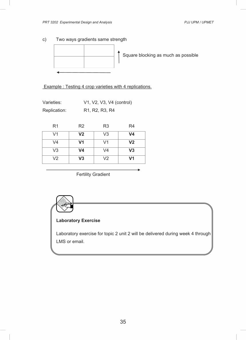
c) Two ways gradients same strength
Square blocking as much as possible
Example : Testing 4 crop varieties with 4 replications.
Varieties: V1, V2, V3, V4 (control)
Replication: R1, R2, R3, R4
R1 R2 R3 R4
V1 V2 V3 V4
V4 V1 V1 V2
V3 V4 V4 V3
V2 V3 V2 V1
Fertility Gradient
Laboratory Exercise
Laboratory exercise for topic 2 unit 2 will be delivered during week 4 through
LMS or email.
35
PRT 3202 Experimental Design and Analysis PJJ UPM / UPMET
18
TOPIC 2: RANDOMIZED COMPLETE BLOCK DESIGN
Important Content In this design treatments are assigned at random to a group of experimental units
called the block. A block consists of uniform experimental units. The main aim of this
design is to keep the variability among experimental units within a block as small as
possible and to maximize differences among the blocks.
.... it is used for an area or location or materials that are heterogeneous
.... group of treatments is placed randomly in a block or replication
.... block or replication is created to reduce the heterogeneity of the experimental
unit
.... each block containing homogenous experimental unit
.... treatments are arranged in each block or replication
.... effect of block is considered in the calculation of ANOVA
Method of blocking in a field
a) One directional gradient
Arrange the block at right angles with the gradient
High Fertility Low Fertility
b) Two ways gradients: 1 strong, 1 less in strength
Moderate
Arrange block perpendicular to the gradient
High Fertility Low Fertility
PRT 3202 Experimental Design and Analysis PJJ UPM / UPMET
19
c) Two ways gradients same strength
Square blocking as much as possible
Example : Testing 4 crop varieties with 4 replications.
Varieties: V1, V2, V3, V4 (control)
Replication: R1, R2, R3, R4
R1 R2 R3 R4
V1 V2 V3 V4
V4 V1 V1 V2
V3 V4 V4 V3
V2 V3 V2 V1
Fertility Gradient
Laboratory Exercise
Laboratory exercise for topic 2 unit 2 will be delivered during week 4 through
LMS or email.

36
PRT 3202 Experimental Design and Analysis PJJ UPM / UPMET
20
TOPIC 3: LATIN SQUARE DESIGN
Important Content
Latin square design handles two known sources of variation among experimental
units simultaneously. It treats the sources as two independent blocking criteria: row-
blocking and column-blocking. This is achieved by making sure that every treatment
occurs only once in each row-block and once in each column-block. This helps to
remove variability from the experimental error associated with both these effects.
• Treatments are arranged in row and column
• Error is being reduced due to two ways heterogeneity (row and column)
• More efficient than RCBD when there is two ways heterogeneity
• Number of replication should be equal to number of treatment
• Usually such arrangement is suitable for 4 to 8 treatments
STEPS IN ARRANGING TREATMENTS WITH RANDOMIZATION IN A LATIN SQURE DESIGN
Example: Effect of 6 different fertilizer N treatments (A, B, C, D, E, and F) on the
yield of corn.
1. Arrange each treatment so that it occurs once in a row and once in a column
only.
Row
Column
B D E F A C
C E A D F B
A F C B E D
D A F C B E
F B D E C A
E C B A D F
PRT 3202 Experimental Design and Analysis PJJ UPM / UPMET
21
1. Use random number table, assign numbering for row and column randomly.
Row Column
4 2 5 1 3 6
1 B D E F A C
3 C E A D F B
5 A F C B E D
4 D A F C B E
2 F B D E C A
6 E C B A D F
2. Arrange the treatments in the field based on the arrangement in the above
table 2.
Row Column
1 2 3 4 5 6
1 F D A B E C
3 E B C F D A
5 D E F C A B
4 C A B D F E
2 B F E A C D
6 A C D E B F
Laboratory Exercise
Laboratory exercise for topic 3 unit 2 will be delivered during week 4 through
LMS or email

37
PRT 3202 Experimental Design and Analysis PJJ UPM / UPMET
20
TOPIC 3: LATIN SQUARE DESIGN
Important Content
Latin square design handles two known sources of variation among experimental
units simultaneously. It treats the sources as two independent blocking criteria: row-
blocking and column-blocking. This is achieved by making sure that every treatment
occurs only once in each row-block and once in each column-block. This helps to
remove variability from the experimental error associated with both these effects.
• Treatments are arranged in row and column
• Error is being reduced due to two ways heterogeneity (row and column)
• More efficient than RCBD when there is two ways heterogeneity
• Number of replication should be equal to number of treatment
• Usually such arrangement is suitable for 4 to 8 treatments
STEPS IN ARRANGING TREATMENTS WITH RANDOMIZATION IN A LATIN SQURE DESIGN
Example: Effect of 6 different fertilizer N treatments (A, B, C, D, E, and F) on the
yield of corn.
1. Arrange each treatment so that it occurs once in a row and once in a column
only.
Row
Column
B D E F A C
C E A D F B
A F C B E D
D A F C B E
F B D E C A
E C B A D F
PRT 3202 Experimental Design and Analysis PJJ UPM / UPMET
21
1. Use random number table, assign numbering for row and column randomly.
Row Column
4 2 5 1 3 6
1 B D E F A C
3 C E A D F B
5 A F C B E D
4 D A F C B E
2 F B D E C A
6 E C B A D F
2. Arrange the treatments in the field based on the arrangement in the above
table 2.
Row Column
1 2 3 4 5 6
1 F D A B E C
3 E B C F D A
5 D E F C A B
4 C A B D F E
2 B F E A C D
6 A C D E B F
Laboratory Exercise
Laboratory exercise for topic 3 unit 2 will be delivered during week 4 through
LMS or email

38
PRT 3202 Experimental Design and Analysis PJJ UPM / UPMET
22
UNIT 3
ANALYSIS OF VARIANCE
Introduction Analysis of variance (ANOVA) is to determine the ratio of between samples to the
variance of within samples that is the F distribution. The value of F is used to reject
or accept the null hypothesis. It is used to analyze the variances of treatments or
events for significant differences between treatment variances, particularly in
situations where more than two treatments are involved. ANOVA can only be used to
ascertain if the treatment differences are significant or not.
Objective To accept or reject the null hypothesis where more than two treatments are involved.
TOPIC 1: F DISTRIBUTION
Important Content F value is used to test the significant difference between more than two treatment
means
F = s2, calculated from sample mean
s2, calculate from variance between individual sample
= sa2 (variance between samples)
sd2 (variance within samples)
df (numerator) = n -1, where n = number of samples
df (denominator) = n(r – 1), where r = size of samples
PRT 3202 Experimental Design and Analysis PJJ UPM / UPMET
23
Laboratory Exercise
Laboratory exercise for topic 1 unit 3 will be delivered during week 5 through
LMS or email.
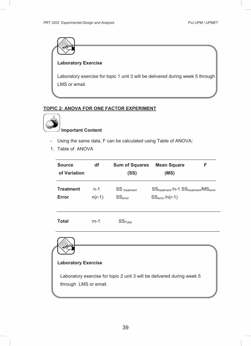
TOPIC 2: ANOVA FOR ONE FACTOR EXPERIMENT
Important Content
- Using the same data, F can be calculated using Table of ANOVA:
1. Table of ANOVA
Source df Sum of Squares Mean Square F of Variation (SS) (MS)
Treatment n-1 SS treatment SStreatment /n-1 SStreatment/MSerror
Error n(r-1) SSerror SSerror /n(r-1)
Total rn-1 SSTotal
Laboratory Exercise
Laboratory exercise for topic 2 unit 3 will be delivered during week 5
through LMS or email.
39
PRT 3202 Experimental Design and Analysis PJJ UPM / UPMET
22
UNIT 3
ANALYSIS OF VARIANCE
Introduction Analysis of variance (ANOVA) is to determine the ratio of between samples to the
variance of within samples that is the F distribution. The value of F is used to reject
or accept the null hypothesis. It is used to analyze the variances of treatments or
events for significant differences between treatment variances, particularly in
situations where more than two treatments are involved. ANOVA can only be used to
ascertain if the treatment differences are significant or not.
Objective To accept or reject the null hypothesis where more than two treatments are involved.
TOPIC 1: F DISTRIBUTION
Important Content F value is used to test the significant difference between more than two treatment
means
F = s2, calculated from sample mean
s2, calculate from variance between individual sample
= sa2 (variance between samples)
sd2 (variance within samples)
df (numerator) = n -1, where n = number of samples
df (denominator) = n(r – 1), where r = size of samples
PRT 3202 Experimental Design and Analysis PJJ UPM / UPMET
23
Laboratory Exercise
Laboratory exercise for topic 1 unit 3 will be delivered during week 5 through
LMS or email.
TOPIC 2: ANOVA FOR ONE FACTOR EXPERIMENT
Important Content
- Using the same data, F can be calculated using Table of ANOVA:
1. Table of ANOVA
Source df Sum of Squares Mean Square F of Variation (SS) (MS)
Treatment n-1 SS treatment SStreatment /n-1 SStreatment/MSerror
Error n(r-1) SSerror SSerror /n(r-1)
Total rn-1 SSTotal
Laboratory Exercise
Laboratory exercise for topic 2 unit 3 will be delivered during week 5
through LMS or email.

40
PRT 3202 Experimental Design and Analysis PJJ UPM / UPMET
24
TOPIC 3: ANOVA FOR VARIOUS DESIGNS
Important Content
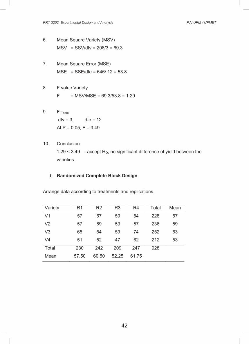
a. Complete Randomized Design Example: Testing yield of 4 varieties with 4 replications.
Varieties: V1, V2, V3, V4 (Control)
Replications: R1, R2, R3, R4
V1R3 (50) V2R2 (69) V1R4 (54) V4R1(51)
V2 R4 (57) V1R2 (67) V3R1 (65) V4R4 (62)
V2R1 (57) V2R3 (53) V4R2 (52) V3R4 (74)
V3R2 (54) V1R1 (57) V4R3 (47) V3R3 (59)
Calculation:
Arrange the data according to treatment and replication
Variety Replication Total Mean
1 2 3 4
V1 57 67 50 54 228 57
V2 57 69 53 57 236 59
V3 65 54 59 74 252 63
V4 51 52 47 62 212 53
Total
928
PRT 3202 Experimental Design and Analysis PJJ UPM / UPMET
25
ANOVA
HO: no significant difference in yield between the varieties.
Table of ANOVA
Source of df SS MS F FTable
Variation (p=0.05)
Variety 3 208 69.3 1.29 3.49
Error 12 646 53.8
Total 15 854
Calculation
1. Degree of Freedom, df
df (total) = vr – 1 = 4(4) – 1 = 15
df (variety) = v – 1 = 4 – 1 = 3
df (error) = df(total) – df(variety) = 15 – 3 = 12
or
df (error) = v(r – 1) = 4(4 – 1) = 12
2. Correction factor, CF
CF = Y..2 / rv = (928)2/(4×4) = 53824
3. Sum Square Total (SST)
SST = ƩYij2 – CF
= (572 + 672 + ... + 472 + 622) – 53824
= 54678 – 53824 = 854
4. Sum Square Variety (SSV)
SSV = (ƩY.j2/ r) – CF
= (2282 + 2362 + 2522 + 2122)/ 4 – 53824
= 54032 – 53824 = 208
5. Sum Square Error (SSE)
SSE = SST – SSV
= 854 – 208 = 646
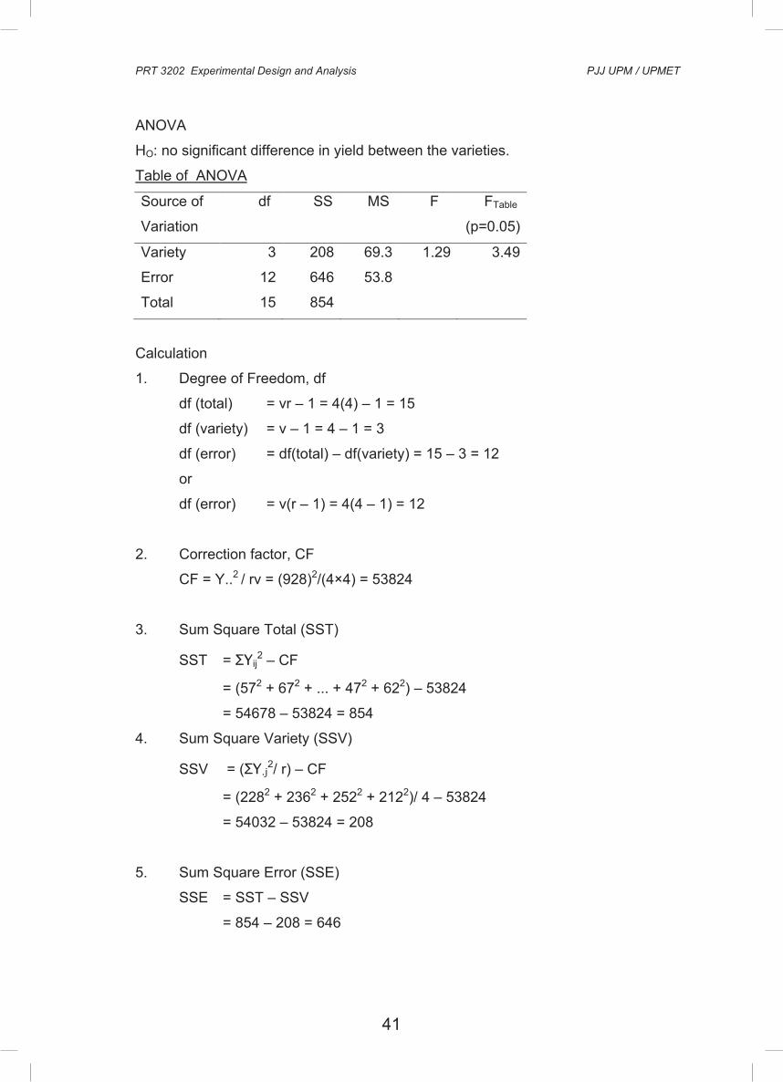
41
PRT 3202 Experimental Design and Analysis PJJ UPM / UPMET
24
TOPIC 3: ANOVA FOR VARIOUS DESIGNS
Important Content
a. Complete Randomized Design Example: Testing yield of 4 varieties with 4 replications.
Varieties: V1, V2, V3, V4 (Control)
Replications: R1, R2, R3, R4
V1R3 (50) V2R2 (69) V1R4 (54) V4R1(51)
V2 R4 (57) V1R2 (67) V3R1 (65) V4R4 (62)
V2R1 (57) V2R3 (53) V4R2 (52) V3R4 (74)
V3R2 (54) V1R1 (57) V4R3 (47) V3R3 (59)
Calculation:
Arrange the data according to treatment and replication
Variety Replication Total Mean
1 2 3 4
V1 57 67 50 54 228 57
V2 57 69 53 57 236 59
V3 65 54 59 74 252 63
V4 51 52 47 62 212 53
Total
928
PRT 3202 Experimental Design and Analysis PJJ UPM / UPMET
25
ANOVA
HO: no significant difference in yield between the varieties.
Table of ANOVA
Source of df SS MS F FTable
Variation (p=0.05)
Variety 3 208 69.3 1.29 3.49
Error 12 646 53.8
Total 15 854
Calculation
1. Degree of Freedom, df
df (total) = vr – 1 = 4(4) – 1 = 15
df (variety) = v – 1 = 4 – 1 = 3
df (error) = df(total) – df(variety) = 15 – 3 = 12
or
df (error) = v(r – 1) = 4(4 – 1) = 12
2. Correction factor, CF
CF = Y..2 / rv = (928)2/(4×4) = 53824
3. Sum Square Total (SST)
SST = ƩYij2 – CF
= (572 + 672 + ... + 472 + 622) – 53824
= 54678 – 53824 = 854
4. Sum Square Variety (SSV)
SSV = (ƩY.j2/ r) – CF
= (2282 + 2362 + 2522 + 2122)/ 4 – 53824
= 54032 – 53824 = 208
5. Sum Square Error (SSE)
SSE = SST – SSV
= 854 – 208 = 646
42
PRT 3202 Experimental Design and Analysis PJJ UPM / UPMET
26
6. Mean Square Variety (MSV)
MSV = SSV/dfv = 208/3 = 69.3
7. Mean Square Error (MSE)
MSE = SSE/dfe = 646/ 12 = 53.8
8. F value Variety
F = MSV/MSE = 69.3/53.8 = 1.29
9. F Table
dfv = 3, dfe = 12
At P = 0.05, F = 3.49
10. Conclusion
1.29 < 3.49 → accept HO, no significant difference of yield between the
varieties.
b. Randomized Complete Block Design
Arrange data according to treatments and replications.
Variety R1 R2 R3 R4 Total Mean
V1 57 67 50 54 228 57
V2 57 69 53 57 236 59
V3 65 54 59 74 252 63
V4 51 52 47 62 212 53
Total 230 242 209 247 928
Mean 57.50 60.50 52.25 61.75
PRT 3202 Experimental Design and Analysis PJJ UPM / UPMET
27
Calculation:
HO: no significant difference of yield between varieties.
Table of ANOVA
Source of df SS MS F FTable
Variation
(p=0.05)
Block (Rep) 3 214.5 71.5 1.49 3.86
Variety 3 208 69.3 1.45 3.86
Error 9 431.5 47.94
Total 15 854
Calculation
1. Degree of Freedom (df)
df (total) = vr – 1 = 4(4) – 1 = 15
df (block) = r – 1 = 4 – 1 = 3
df (variety) = v – 1 = 4 – 1 = 3
df (error) = df (total) – df(block) – df(variety)
= 15 – 3 – 3 = 9 Or
df (error) = (v-1)(r-1) = (4-1)(4-1) = 9
2. Correction Factor, CF
CF = Y..2/rv = (928)2/ (4×4) = 53824
3. Sum Square Total (SST)
SST = ƩYij2 – CF
= (572 + 672 + ... + 472 + 622) – 53824
= 54678 – 53824 = 854
4. Sum Square Block (SSB)
SSB = (Ʃy.j2/v) – CF
= (2302 + 2422 + 2092 + 2472)/ 4 – 53824
= 54038.5 – 53824 = 214.5
43
PRT 3202 Experimental Design and Analysis PJJ UPM / UPMET
26
6. Mean Square Variety (MSV)
MSV = SSV/dfv = 208/3 = 69.3
7. Mean Square Error (MSE)
MSE = SSE/dfe = 646/ 12 = 53.8
8. F value Variety
F = MSV/MSE = 69.3/53.8 = 1.29
9. F Table
dfv = 3, dfe = 12
At P = 0.05, F = 3.49
10. Conclusion
1.29 < 3.49 → accept HO, no significant difference of yield between the
varieties.
b. Randomized Complete Block Design
Arrange data according to treatments and replications.
Variety R1 R2 R3 R4 Total Mean
V1 57 67 50 54 228 57
V2 57 69 53 57 236 59
V3 65 54 59 74 252 63
V4 51 52 47 62 212 53
Total 230 242 209 247 928
Mean 57.50 60.50 52.25 61.75
PRT 3202 Experimental Design and Analysis PJJ UPM / UPMET
27
Calculation:
HO: no significant difference of yield between varieties.
Table of ANOVA
Source of df SS MS F FTable
Variation
(p=0.05)
Block (Rep) 3 214.5 71.5 1.49 3.86
Variety 3 208 69.3 1.45 3.86
Error 9 431.5 47.94
Total 15 854
Calculation
1. Degree of Freedom (df)
df (total) = vr – 1 = 4(4) – 1 = 15
df (block) = r – 1 = 4 – 1 = 3
df (variety) = v – 1 = 4 – 1 = 3
df (error) = df (total) – df(block) – df(variety)
= 15 – 3 – 3 = 9 Or
df (error) = (v-1)(r-1) = (4-1)(4-1) = 9
2. Correction Factor, CF
CF = Y..2/rv = (928)2/ (4×4) = 53824
3. Sum Square Total (SST)
SST = ƩYij2 – CF
= (572 + 672 + ... + 472 + 622) – 53824
= 54678 – 53824 = 854
4. Sum Square Block (SSB)
SSB = (Ʃy.j2/v) – CF
= (2302 + 2422 + 2092 + 2472)/ 4 – 53824
= 54038.5 – 53824 = 214.5

44
PRT 3202 Experimental Design and Analysis PJJ UPM / UPMET
28
5. Sum Square Variety (SSV)
SSV = (ƩYi.2/r) – CF
= (2282 + 2362 + 2522 + 2122)/4 – 53824
= 54032 – 53824 = 208
6. Sum Square Error (SSE)
SSE = SST – SSB – SSV
= 854 – 214.5 – 208 = 431.5
7. Mean Square Blok (MSB)
MSB = SSB/dfb = 214.5/3 = 71.5
8. Mean Square Variety (MSV)
MSV = SSV/dfv = 208/3 = 69.3
9. Mean Square Error (MSE)
MSE = SSE/dfe = 431.5/9 = 47.94
10. F value
F value (block) = MSB/MSE = 71.5/47.94 = 1.49
F (variety) = MSV/MSE = 69.3/47.94 = 1.45
11. F Table
Block: dfb = 3, dfe = 9, at p = 0.05, F = 3.86
Variety: dfv = 3, dfe = 9, at p = 0.05, F = 8.91
12. Conclusion
Variety: 1.45 < 3.86 → accept HO, there is no significant different between varieties
on yield.
Block: 1.49 < 3.86 → accept HO, there is no significant effect of block on the yield.
PRT 3202 Experimental Design and Analysis PJJ UPM / UPMET
29
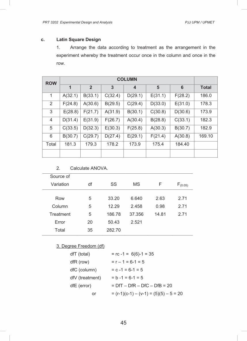
c. Latin Square Design 1. Arrange the data according to treatment as the arrangement in the
experiment whereby the treatment occur once in the column and once in the
row.
ROW COLUMN
1 2 3 4 5 6 Total
1 A(32.1) B(33.1) C(32.4) D(29.1) E(31.1) F(28.2) 186.0
2 F(24.8) A(30.6) B(29.5) C(29.4) D(33.0) E(31.0) 178.3
3 E(28.8) F(21.7) A(31.9) B(30.1) C(30.8) D(30.6) 173.9
4 D(31.4) E(31.9) F(26.7) A(30.4) B(28.8) C(33.1) 182.3
5 C(33.5) D(32.3) E(30.3) F(25.8) A(30.3) B(30.7) 182.9
6 B(30.7) C(29.7) D(27.4) E(29.1) F(21.4) A(30.8) 169.10
Total 181.3 179.3 178.2 173.9 175.4 184.40
2. Calculate ANOVA.
Source of
Variation df SS MS F F(0.05)
Row 5 33.20 6.640 2.63 2.71
Column 5 12.29 2.458 0.98 2.71
Treatment 5 186.78 37.356 14.81 2.71
Error 20 50.43 2.521
Total 35 282.70
3. Degree Freedom (df)
dfT (total) = rc -1 = 6(6)-1 = 35
dfR (row) = r – 1 = 6-1 = 5
dfC (column) = c -1 = 6-1 = 5
dfV (treatment) = b -1 = 6-1 = 5
dfE (error) = DfT – DfR – DfC – DfB = 20
or = (r-1)(c-1) – (v-1) = (5)(5) – 5 = 20
45
PRT 3202 Experimental Design and Analysis PJJ UPM / UPMET
28
5. Sum Square Variety (SSV)
SSV = (ƩYi.2/r) – CF
= (2282 + 2362 + 2522 + 2122)/4 – 53824
= 54032 – 53824 = 208
6. Sum Square Error (SSE)
SSE = SST – SSB – SSV
= 854 – 214.5 – 208 = 431.5
7. Mean Square Blok (MSB)
MSB = SSB/dfb = 214.5/3 = 71.5
8. Mean Square Variety (MSV)
MSV = SSV/dfv = 208/3 = 69.3
9. Mean Square Error (MSE)
MSE = SSE/dfe = 431.5/9 = 47.94
10. F value
F value (block) = MSB/MSE = 71.5/47.94 = 1.49
F (variety) = MSV/MSE = 69.3/47.94 = 1.45
11. F Table
Block: dfb = 3, dfe = 9, at p = 0.05, F = 3.86
Variety: dfv = 3, dfe = 9, at p = 0.05, F = 8.91
12. Conclusion
Variety: 1.45 < 3.86 → accept HO, there is no significant different between varieties
on yield.
Block: 1.49 < 3.86 → accept HO, there is no significant effect of block on the yield.
PRT 3202 Experimental Design and Analysis PJJ UPM / UPMET
29
c. Latin Square Design 1. Arrange the data according to treatment as the arrangement in the
experiment whereby the treatment occur once in the column and once in the
row.
ROW COLUMN
1 2 3 4 5 6 Total
1 A(32.1) B(33.1) C(32.4) D(29.1) E(31.1) F(28.2) 186.0
2 F(24.8) A(30.6) B(29.5) C(29.4) D(33.0) E(31.0) 178.3
3 E(28.8) F(21.7) A(31.9) B(30.1) C(30.8) D(30.6) 173.9
4 D(31.4) E(31.9) F(26.7) A(30.4) B(28.8) C(33.1) 182.3
5 C(33.5) D(32.3) E(30.3) F(25.8) A(30.3) B(30.7) 182.9
6 B(30.7) C(29.7) D(27.4) E(29.1) F(21.4) A(30.8) 169.10
Total 181.3 179.3 178.2 173.9 175.4 184.40
2. Calculate ANOVA.
Source of
Variation df SS MS F F(0.05)
Row 5 33.20 6.640 2.63 2.71
Column 5 12.29 2.458 0.98 2.71
Treatment 5 186.78 37.356 14.81 2.71
Error 20 50.43 2.521
Total 35 282.70
3. Degree Freedom (df)
dfT (total) = rc -1 = 6(6)-1 = 35
dfR (row) = r – 1 = 6-1 = 5
dfC (column) = c -1 = 6-1 = 5
dfV (treatment) = b -1 = 6-1 = 5
dfE (error) = DfT – DfR – DfC – DfB = 20
or = (r-1)(c-1) – (v-1) = (5)(5) – 5 = 20

46
PRT 3202 Experimental Design and Analysis PJJ UPM / UPMET
30
4. Correction Factor, CF
CF = Y...2 / rc
= (1072.5)2 / 6(6)
= 31951.56
5. Sum of Square (SS) and Mean Square (MS)
Total SST = ƩY2… – CF
= 32.12 + 33.12 + .... + 21.42 + 30.82 – 31951.56
= 282.70
Row SSR = Ʃyi..2/c – CF
= (186.02 +.... + 169.12)/6 – 31903.91
= 33..20
MSR = SSR/DfR = 33.20/5
= 6.64
Column SSC = Ʃy.j.2/r – CF
= (181.32 + ... + 184.42)/6 – 31951.56
= 12.29
MSC = SSC/DfC = 12.29/5
= 2.458
Treatment (V)
SSV = Ʃy..K2/rep – CF
= (186.12 + ... + 148.62)/6 – 31951.56
= 186.78
MSB = SSV/DfV = 186.78/5
= 37.356
Error SSE = SST – SSR – SSC – SSV
= 282.70 – 33.20 – 12.29 – 186.78
= 50.43
MSE = SSE/DFE = 50.43/20
= 2.521
PRT 3202 Experimental Design and Analysis PJJ UPM / UPMET
31
6. F value
F (row) = MSR/MSE = 6.640/2.521 = 2.63
F (Column) = MSC/MSE = 2.458/2.521 = 0.98
F (Treatment) = MSV/MSE = 37.356/2.521 =14.81
7. Table F value
Rows: dfR = 5, dfE = 20, p = 0.05 F = 2.71
Column:dfC = 5, dfE = 20, p = 0.05 F = 2.71
Treatment:dfV = 5, dfE = 20, p = 0.05 F = 2.71
Conclusion Treatment: F (14.81) > F table (2.71) Reject HO, there is at least one
significant difference between the treatments.
Row: F value (2.63) < F table (2.71) accept HO, there is no significant
difference between the rows.
Column: F value (0.98) < F table (2.71) accept HO, there is no significant
different between columns.
Laboratory Exercise
Laboratory exercise for topic 3 unit 3 will be delivered during week 5 through
LMS or email.

47
PRT 3202 Experimental Design and Analysis PJJ UPM / UPMET
30
4. Correction Factor, CF
CF = Y...2 / rc
= (1072.5)2 / 6(6)
= 31951.56
5. Sum of Square (SS) and Mean Square (MS)
Total SST = ƩY2… – CF
= 32.12 + 33.12 + .... + 21.42 + 30.82 – 31951.56
= 282.70
Row SSR = Ʃyi..2/c – CF
= (186.02 +.... + 169.12)/6 – 31903.91
= 33..20
MSR = SSR/DfR = 33.20/5
= 6.64
Column SSC = Ʃy.j.2/r – CF
= (181.32 + ... + 184.42)/6 – 31951.56
= 12.29
MSC = SSC/DfC = 12.29/5
= 2.458
Treatment (V)
SSV = Ʃy..K2/rep – CF
= (186.12 + ... + 148.62)/6 – 31951.56
= 186.78
MSB = SSV/DfV = 186.78/5
= 37.356
Error SSE = SST – SSR – SSC – SSV
= 282.70 – 33.20 – 12.29 – 186.78
= 50.43
MSE = SSE/DFE = 50.43/20
= 2.521
PRT 3202 Experimental Design and Analysis PJJ UPM / UPMET
31
6. F value
F (row) = MSR/MSE = 6.640/2.521 = 2.63
F (Column) = MSC/MSE = 2.458/2.521 = 0.98
F (Treatment) = MSV/MSE = 37.356/2.521 =14.81
7. Table F value
Rows: dfR = 5, dfE = 20, p = 0.05 F = 2.71
Column:dfC = 5, dfE = 20, p = 0.05 F = 2.71
Treatment:dfV = 5, dfE = 20, p = 0.05 F = 2.71
Conclusion Treatment: F (14.81) > F table (2.71) Reject HO, there is at least one
significant difference between the treatments.
Row: F value (2.63) < F table (2.71) accept HO, there is no significant
difference between the rows.
Column: F value (0.98) < F table (2.71) accept HO, there is no significant
different between columns.
Laboratory Exercise
Laboratory exercise for topic 3 unit 3 will be delivered during week 5 through
LMS or email.

48
PRT 3202 Experimental Design and Analysis PJJ UPM / UPMET
32
UNIT 4
COMPARISON OF TREATMENT MEANS
Introduction
Comparison of means is conducted when the null hypothesis (HO ) is being rejected
during the process of ANOVA. When HO is rejected, there is at least one significant
difference between the treatment means. There are various methods to compare for
significant difference between the treatments means. The means of more than two
means are often compared for significant difference using Least Significant
Difference (LSD) test, Duncan’s New Multiple Range (DMRT) test, Tukey’s test,
Scheffe’s test, Student –Newman-Keul’s test (SNK), Dunnett’s test and Contrast.
However, more often than not, such tests are misused. One of the main reasons for
this is the lack of clear understanding of what pair and group comparisons as well as
what the structure of treatments under investigation are. There are two types of pair
comparison namely planned and unplanned pair.
Objective To compare between the treatment means after rejecting the HO from ANOVA.
PRT 3202 Experimental Design and Analysis PJJ UPM / UPMET
33
TOPIC 1: Least Significant Difference (LSD)
Important Content It is a t-test and usually suitable to compare between two means.
Example:
Source of df SS MS F Ftable
Variation
(p=0.05)
Block (Rep) 3 576 192 24.7 3.86
Variety 3 208 69.3 8.9 3.86
Error 9 70 7.78
Total 15 854
Arrange the means from low to high or from high to low
Variety V4 V1 V2 V3
Mean 53 57 59 63
Calculation
T = (d - µd) / sd
D = Y1 – Y2
Assume the mean are from the same population, so µd = 0
t = d/sd
t = LSD/ sd
LSD = t. sd
sd = √2MSE/r
sd = √2(7.78) /4 = 1.972
obtain t value from table df = dfe = 9, p = 0.05
t = 2.262
LSD = 2.262 × 1.972 = 4.46 t ha-1

49
PRT 3202 Experimental Design and Analysis PJJ UPM / UPMET
32
UNIT 4
COMPARISON OF TREATMENT MEANS
Introduction
Comparison of means is conducted when the null hypothesis (HO ) is being rejected
during the process of ANOVA. When HO is rejected, there is at least one significant
difference between the treatment means. There are various methods to compare for
significant difference between the treatments means. The means of more than two
means are often compared for significant difference using Least Significant
Difference (LSD) test, Duncan’s New Multiple Range (DMRT) test, Tukey’s test,
Scheffe’s test, Student –Newman-Keul’s test (SNK), Dunnett’s test and Contrast.
However, more often than not, such tests are misused. One of the main reasons for
this is the lack of clear understanding of what pair and group comparisons as well as
what the structure of treatments under investigation are. There are two types of pair
comparison namely planned and unplanned pair.
Objective To compare between the treatment means after rejecting the HO from ANOVA.
PRT 3202 Experimental Design and Analysis PJJ UPM / UPMET
33
TOPIC 1: Least Significant Difference (LSD)
Important Content It is a t-test and usually suitable to compare between two means.
Example:
Source of df SS MS F Ftable
Variation
(p=0.05)
Block (Rep) 3 576 192 24.7 3.86
Variety 3 208 69.3 8.9 3.86
Error 9 70 7.78
Total 15 854
Arrange the means from low to high or from high to low
Variety V4 V1 V2 V3
Mean 53 57 59 63
Calculation
T = (d - µd) / sd
D = Y1 – Y2
Assume the mean are from the same population, so µd = 0
t = d/sd
t = LSD/ sd
LSD = t. sd
sd = √2MSE/r
sd = √2(7.78) /4 = 1.972
obtain t value from table df = dfe = 9, p = 0.05
t = 2.262
LSD = 2.262 × 1.972 = 4.46 t ha-1
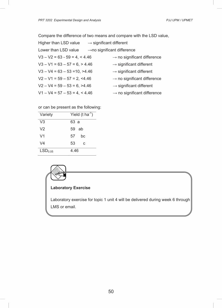
50
PRT 3202 Experimental Design and Analysis PJJ UPM / UPMET
34
Compare the difference of two means and compare with the LSD value,
Higher than LSD value → significant different
Lower than LSD value →no significant difference
V3 – V2 = 63 - 59 = 4, < 4.46 → no significant difference
V3 – V1 = 63 – 57 = 6, > 4.46 → significant different
V3 – V4 = 63 – 53 =10, >4.46 → significant different
V2 – V1 = 59 – 57 = 2, <4.46 → no significant difference
V2 – V4 = 59 – 53 = 6, >4.46 → significant different
V1 – V4 = 57 – 53 = 4, < 4.46 → no significant difference
or can be present as the following:
Variety Yield (t ha-1)
V3 63 a
V2 59 ab
V1 57 bc
V4 53 c
LSD0.05 4.46
Laboratory Exercise
Laboratory exercise for topic 1 unit 4 will be delivered during week 6 through
LMS or email.
PRT 3202 Experimental Design and Analysis PJJ UPM / UPMET
35
TOPIC 2: DUNCAN’S MULTIPLE RANGE TEST
Important Content To compare between treatments means for multiple comparison.
Calculation
1. Calculate LSD value
LSD0.05 = t √2MSE/r = 2.262√2(7.78)/4 = 4.46
2. Calculate D value
D = R(LSD)
R from table, that is up to 4 levels of comparison
Level of Comparison 2 3 4
R0.05 value 1 1.04 1.07
D = R(LSD) 4.46 4.64 4.77
2. Arrange the means from small to high
V4 V1 V2 V3
53 57 59 63
a
b
c
Compare the means of the highest and the lowest first, the difference is compared
with D. The value of D will depend on the level of the means
Example:
V3 – V4, compare with D at level 4 -1 + 1 =4, D = 4.77
V2 – V1, compare with D at level 3 -2 + 1 =2, D = 4.46
V3 vs V4 = 63-53 = 10 > 4.77 → significant different
V3 vs V1 = 63-57 = 6 > 4.64 → significant different
V3 vs V2 = 63-59 = 4 < 4.46 → no significant different

51
PRT 3202 Experimental Design and Analysis PJJ UPM / UPMET
34
Compare the difference of two means and compare with the LSD value,
Higher than LSD value → significant different
Lower than LSD value →no significant difference
V3 – V2 = 63 - 59 = 4, < 4.46 → no significant difference
V3 – V1 = 63 – 57 = 6, > 4.46 → significant different
V3 – V4 = 63 – 53 =10, >4.46 → significant different
V2 – V1 = 59 – 57 = 2, <4.46 → no significant difference
V2 – V4 = 59 – 53 = 6, >4.46 → significant different
V1 – V4 = 57 – 53 = 4, < 4.46 → no significant difference
or can be present as the following:
Variety Yield (t ha-1)
V3 63 a
V2 59 ab
V1 57 bc
V4 53 c
LSD0.05 4.46
Laboratory Exercise
Laboratory exercise for topic 1 unit 4 will be delivered during week 6 through
LMS or email.
PRT 3202 Experimental Design and Analysis PJJ UPM / UPMET
35
TOPIC 2: DUNCAN’S MULTIPLE RANGE TEST
Important Content To compare between treatments means for multiple comparison.
Calculation
1. Calculate LSD value
LSD0.05 = t √2MSE/r = 2.262√2(7.78)/4 = 4.46
2. Calculate D value
D = R(LSD)
R from table, that is up to 4 levels of comparison
Level of Comparison 2 3 4
R0.05 value 1 1.04 1.07
D = R(LSD) 4.46 4.64 4.77
2. Arrange the means from small to high
V4 V1 V2 V3
53 57 59 63
a
b
c
Compare the means of the highest and the lowest first, the difference is compared
with D. The value of D will depend on the level of the means
Example:
V3 – V4, compare with D at level 4 -1 + 1 =4, D = 4.77
V2 – V1, compare with D at level 3 -2 + 1 =2, D = 4.46
V3 vs V4 = 63-53 = 10 > 4.77 → significant different
V3 vs V1 = 63-57 = 6 > 4.64 → significant different
V3 vs V2 = 63-59 = 4 < 4.46 → no significant different
52
PRT 3202 Experimental Design and Analysis PJJ UPM / UPMET
36
Use the same letter for non-significant difference between the means and then
continues in comparing between the second highest mean with the lowest and so on.
Present the result as the following:
Variety Yield (t ha-1)
V3 63 a
V2 59 ab
V1 57 bc
V4 53 c
Means with the same letter is not significantly different according to DNMRT at p=
0.05.
Laboratory Exercise
Laboratory exercise for topic 2 unit 4 will be delivered during week 6 through
LMS or email.
TOPIC 3: CONTRAST
Important Content
One of the methods of comparison between treatments means and also between
groups of means with df value of 1.
PRT 3202 Experimental Design and Analysis PJJ UPM / UPMET
37
Example 4 varieties of sweet potato are tested using a RCBD design with 4
replications.
Variety Type of plant Leaf
V1 Creeper (M) Wide (L)
V2 M Small (K)
V3 Cluster (R) L
V4 R K
Results
Variety Rep 1 Rep 2 Rep 3 Rep 4 Total
V1 47 52 62 51 212
V2 50 64 67 57 228
V3 57 53 69 57 236
V4 54 65 74 59 252
Total
928
Table of ANOVA
Source of
Variation df SS MS F Ftable
Replication 3 576 192 24.7 3.86
Variety 3 208 69.3 8.9 3.86
Error 9 70 7.78
Total 15 854
Comparison
1. Is creeping variety and cluster variety produced the same yield?
2. Are variety with wide and small leaves produced the same yield?
3. Is variety with wide leaf suitable with creeping than variety with small leaf and
cluster?
I
This can be answered with orthogonal contrast, how?
1. Create table for orthogonal coefficient (c)
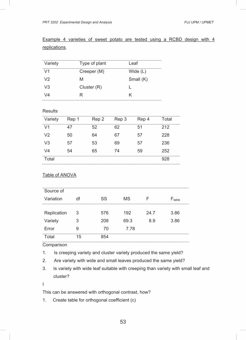
53
PRT 3202 Experimental Design and Analysis PJJ UPM / UPMET
36
Use the same letter for non-significant difference between the means and then
continues in comparing between the second highest mean with the lowest and so on.
Present the result as the following:
Variety Yield (t ha-1)
V3 63 a
V2 59 ab
V1 57 bc
V4 53 c
Means with the same letter is not significantly different according to DNMRT at p=
0.05.
Laboratory Exercise
Laboratory exercise for topic 2 unit 4 will be delivered during week 6 through
LMS or email.
TOPIC 3: CONTRAST
Important Content
One of the methods of comparison between treatments means and also between
groups of means with df value of 1.
PRT 3202 Experimental Design and Analysis PJJ UPM / UPMET
37
Example 4 varieties of sweet potato are tested using a RCBD design with 4
replications.
Variety Type of plant Leaf
V1 Creeper (M) Wide (L)
V2 M Small (K)
V3 Cluster (R) L
V4 R K
Results
Variety Rep 1 Rep 2 Rep 3 Rep 4 Total
V1 47 52 62 51 212
V2 50 64 67 57 228
V3 57 53 69 57 236
V4 54 65 74 59 252
Total
928
Table of ANOVA
Source of
Variation df SS MS F Ftable
Replication 3 576 192 24.7 3.86
Variety 3 208 69.3 8.9 3.86
Error 9 70 7.78
Total 15 854
Comparison
1. Is creeping variety and cluster variety produced the same yield?
2. Are variety with wide and small leaves produced the same yield?
3. Is variety with wide leaf suitable with creeping than variety with small leaf and
cluster?
I
This can be answered with orthogonal contrast, how?
1. Create table for orthogonal coefficient (c)
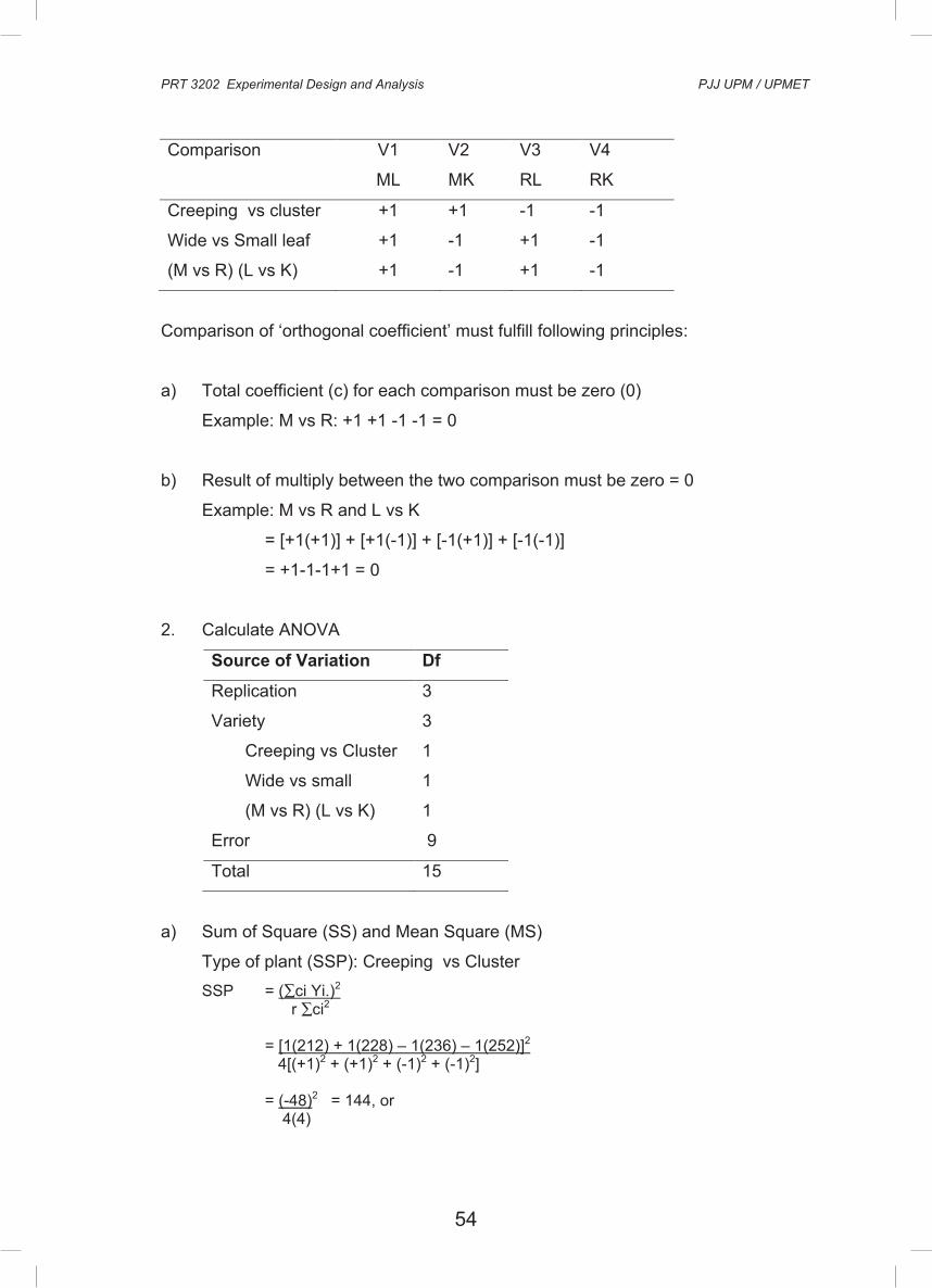
54
PRT 3202 Experimental Design and Analysis PJJ UPM / UPMET
38
Comparison V1 V2 V3 V4
ML MK RL RK
Creeping vs cluster +1 +1 -1 -1
Wide vs Small leaf +1 -1 +1 -1
(M vs R) (L vs K) +1 -1 +1 -1
Comparison of ‘orthogonal coefficient’ must fulfill following principles:
a) Total coefficient (c) for each comparison must be zero (0)
Example: M vs R: +1 +1 -1 -1 = 0
b) Result of multiply between the two comparison must be zero = 0
Example: M vs R and L vs K
= [+1(+1)] + [+1(-1)] + [-1(+1)] + [-1(-1)]
= +1-1-1+1 = 0
2. Calculate ANOVA
Source of Variation Df
Replication 3
Variety 3
Creeping vs Cluster 1
Wide vs small 1
(M vs R) (L vs K) 1
Error 9
Total 15
a) Sum of Square (SS) and Mean Square (MS)
Type of plant (SSP): Creeping vs Cluster SSP = (∑ci Yi.)2
r ∑ci2
= [1(212) + 1(228) – 1(236) – 1(252)]2 4[(+1)2 + (+1)2 + (-1)2 + (-1)2]
= (-48)2 = 144, or 4(4)
PRT 3202 Experimental Design and Analysis PJJ UPM / UPMET
39
SSP = [(212 + 228)2 + (236 + 252)2 – CF 4(2)
CF = (928)2/4(4) = 53824 = 144
MSP = SSP/dfP = 144/1 = 144
Size of leaf (SSL): Wide vs Small
SSD = (∑ci Yi.)2
r ∑ci2
= [1(212) - 1(228) + 1(236) – 1(252)]2
4[(+1)2 + (-1)2 + (+1)2 + (-1)2]
= 64, Or
= (212 + 236)2 + (228 + 252)2 – CF
4(2)
= 64
MSD = SSD/dfD = 64/1 = 64
Interaction between type of plant and size of leaf (SSI): (M vs R)(L vs K) SSI = (∑ci Yi.)2 r ∑ci2
= [1(212) - 1(228) – 1(236) + 1(252)]2 4[(+1)2 + (-1)2 + (-1)2 + (+1)2] = 0, or = (212 + 252)2 + (228 + 236)2 – CF 4(2) = 0 MSI = SSI/dfI = 0/1 = 0 F value
Type of plant: F = MSP/MSE = 144/7.78 = 18.5
Size of leaf: F = MSD/MSE = 64/7.78 = 8.2
Interaction: F = MSI/ dfI = 0/1 = 0
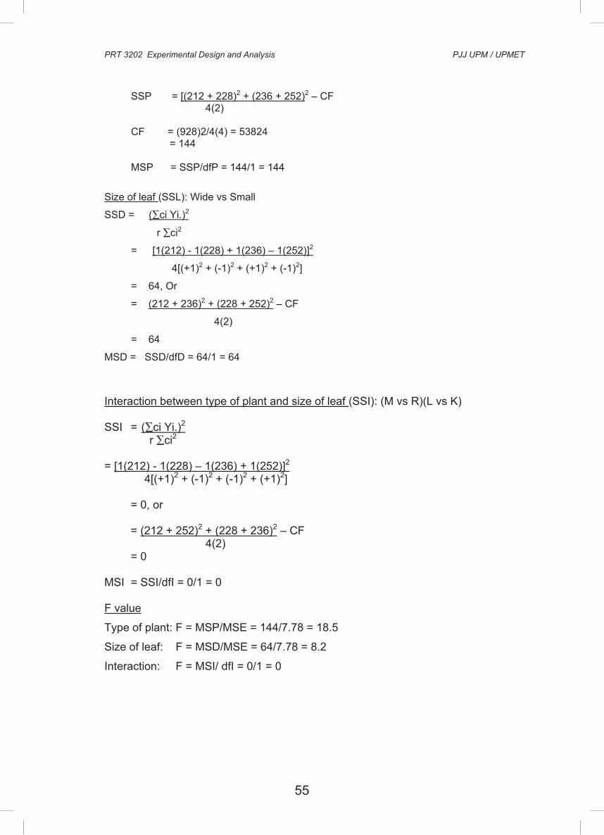
55
PRT 3202 Experimental Design and Analysis PJJ UPM / UPMET
38
Comparison V1 V2 V3 V4
ML MK RL RK
Creeping vs cluster +1 +1 -1 -1
Wide vs Small leaf +1 -1 +1 -1
(M vs R) (L vs K) +1 -1 +1 -1
Comparison of ‘orthogonal coefficient’ must fulfill following principles:
a) Total coefficient (c) for each comparison must be zero (0)
Example: M vs R: +1 +1 -1 -1 = 0
b) Result of multiply between the two comparison must be zero = 0
Example: M vs R and L vs K
= [+1(+1)] + [+1(-1)] + [-1(+1)] + [-1(-1)]
= +1-1-1+1 = 0
2. Calculate ANOVA
Source of Variation Df
Replication 3
Variety 3
Creeping vs Cluster 1
Wide vs small 1
(M vs R) (L vs K) 1
Error 9
Total 15
a) Sum of Square (SS) and Mean Square (MS)
Type of plant (SSP): Creeping vs Cluster SSP = (∑ci Yi.)2
r ∑ci2
= [1(212) + 1(228) – 1(236) – 1(252)]2 4[(+1)2 + (+1)2 + (-1)2 + (-1)2]
= (-48)2 = 144, or 4(4)
PRT 3202 Experimental Design and Analysis PJJ UPM / UPMET
39
SSP = [(212 + 228)2 + (236 + 252)2 – CF 4(2)
CF = (928)2/4(4) = 53824 = 144
MSP = SSP/dfP = 144/1 = 144
Size of leaf (SSL): Wide vs Small
SSD = (∑ci Yi.)2
r ∑ci2
= [1(212) - 1(228) + 1(236) – 1(252)]2
4[(+1)2 + (-1)2 + (+1)2 + (-1)2]
= 64, Or
= (212 + 236)2 + (228 + 252)2 – CF
4(2)
= 64
MSD = SSD/dfD = 64/1 = 64
Interaction between type of plant and size of leaf (SSI): (M vs R)(L vs K) SSI = (∑ci Yi.)2 r ∑ci2
= [1(212) - 1(228) – 1(236) + 1(252)]2 4[(+1)2 + (-1)2 + (-1)2 + (+1)2] = 0, or = (212 + 252)2 + (228 + 236)2 – CF 4(2) = 0 MSI = SSI/dfI = 0/1 = 0 F value
Type of plant: F = MSP/MSE = 144/7.78 = 18.5
Size of leaf: F = MSD/MSE = 64/7.78 = 8.2
Interaction: F = MSI/ dfI = 0/1 = 0
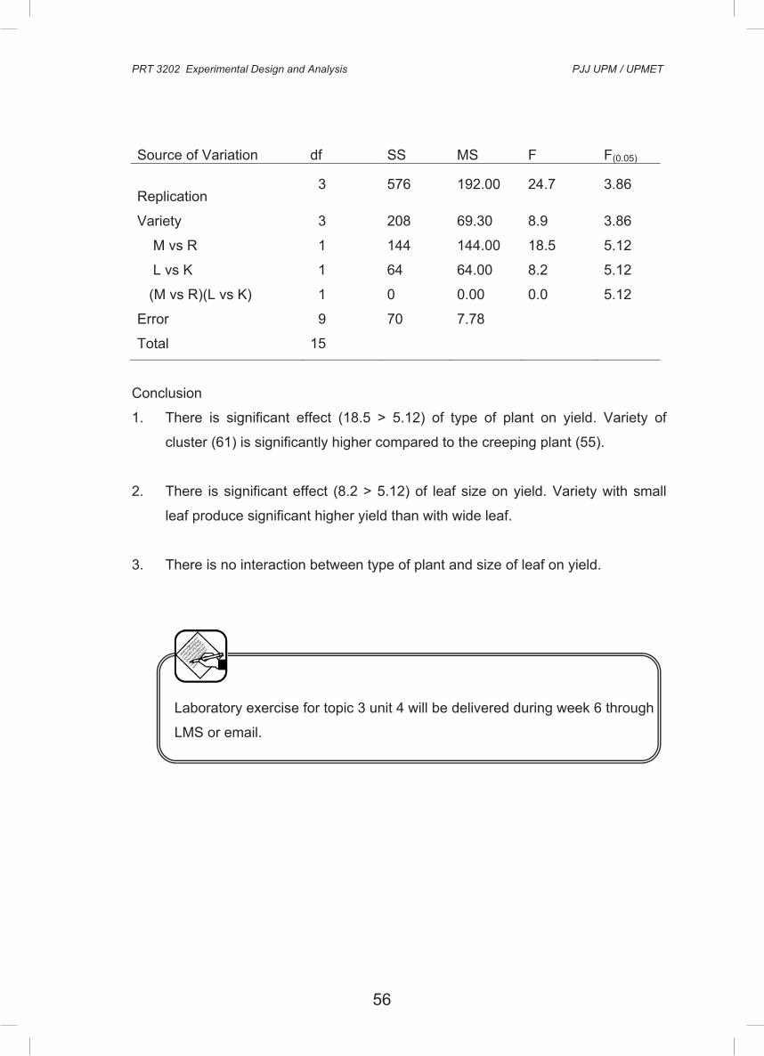
56
PRT 3202 Experimental Design and Analysis PJJ UPM / UPMET
40
Source of Variation df SS MS F F(0.05)
Replication 3 576 192.00 24.7 3.86
Variety 3 208 69.30 8.9 3.86
M vs R 1 144 144.00 18.5 5.12
L vs K 1 64 64.00 8.2 5.12
(M vs R)(L vs K) 1 0 0.00 0.0 5.12
Error 9 70 7.78
Total 15
Conclusion
1. There is significant effect (18.5 > 5.12) of type of plant on yield. Variety of
cluster (61) is significantly higher compared to the creeping plant (55).
2. There is significant effect (8.2 > 5.12) of leaf size on yield. Variety with small
leaf produce significant higher yield than with wide leaf.
3. There is no interaction between type of plant and size of leaf on yield.
Laboratory exercise for topic 3 unit 4 will be delivered during week 6 through
LMS or email.
PRT 3202 Experimental Design and Analysis PJJ UPM / UPMET
41
UNIT 5
DATA TRANSFORMATION
Introduction
Data that are not conformed to normal distribution need to be transformed to
normalize the data. Usually discrete data are required to be transformed so that
various statistical analyses can be carried out.
Objective To transform data using various methods to normalize the data.
TOPIC 1: LOG TRANSFORMATION
Important Content Log transformation is conducted when the variance or standard deviation increase
proportional to the mean that is an increasing standard deviation with a
corresponding increasing mean.
Example :
- Number of insects per plot
- Number of eggs of insect per plant
- Number of leaves per plant
If there is zero (0), convert all the data to lo log (x + 1).
57
PRT 3202 Experimental Design and Analysis PJJ UPM / UPMET
40
Source of Variation df SS MS F F(0.05)
Replication 3 576 192.00 24.7 3.86
Variety 3 208 69.30 8.9 3.86
M vs R 1 144 144.00 18.5 5.12
L vs K 1 64 64.00 8.2 5.12
(M vs R)(L vs K) 1 0 0.00 0.0 5.12
Error 9 70 7.78
Total 15
Conclusion
1. There is significant effect (18.5 > 5.12) of type of plant on yield. Variety of
cluster (61) is significantly higher compared to the creeping plant (55).
2. There is significant effect (8.2 > 5.12) of leaf size on yield. Variety with small
leaf produce significant higher yield than with wide leaf.
3. There is no interaction between type of plant and size of leaf on yield.
Laboratory exercise for topic 3 unit 4 will be delivered during week 6 through
LMS or email.
PRT 3202 Experimental Design and Analysis PJJ UPM / UPMET
41
UNIT 5
DATA TRANSFORMATION
Introduction
Data that are not conformed to normal distribution need to be transformed to
normalize the data. Usually discrete data are required to be transformed so that
various statistical analyses can be carried out.
Objective To transform data using various methods to normalize the data.
TOPIC 1: LOG TRANSFORMATION
Important Content Log transformation is conducted when the variance or standard deviation increase
proportional to the mean that is an increasing standard deviation with a
corresponding increasing mean.
Example :
- Number of insects per plot
- Number of eggs of insect per plant
- Number of leaves per plant
If there is zero (0), convert all the data to lo log (x + 1).
58
PRT 3202 Experimental Design and Analysis PJJ UPM / UPMET
42
Laboratory exercise for topic 1 unit 5 will be delivered during week 7 through
LMS or email.
TOPIC 2 : SQUARE ROOT TRANSFORMATION
Important Content Square root transformation is conducted for low value data or occurrence of a unique
/ weird situation. The square-root transformation is also suitable for percentage with
a range of 0 – 30% and 70 – 100%.
Example:
- Number of plants with diseases
- Number of weed per plot
- Number of infested plants in a plot
If there is zero (0), use square root of (x + 0.5)
Laboratory exercise for topic 2 unit 5 will be delivered during week 7 through
LMS or email.
PRT 3202 Experimental Design and Analysis PJJ UPM / UPMET
43
TOPIC 3 : ARCSINE TRANSFORMATION
Important Content
Arcsine transformation is conducted for ratio, data obtained from counting and
data expressed as decimal fractions or percentages.
For percentage:
It is necessary to transform to arcsine when the percentage range is more than 40
(that is between the smallest data and the highest data).
Example:
Smallest data = 2% and highest data = 82%
Difference = 82 – 2 = 80%, so arcsine is necessary
or Criteria 1: If percentage data fall between 30 – 70, no transformation required Criteria 2: If percentages fall between 0 – 30 or 70 – 100, use square root transformation. Criteria 3: If it did not qualifies for criteria 1 and 3, use arcsine When there is zero (0), change to (1/4n) and when there is100 change to [100 – (1/4n)] before changing all the data to arcsine.
Laboratory exercise for topic 3 unit 5 will be delivered during week 7 through
LMS or email.
59
PRT 3202 Experimental Design and Analysis PJJ UPM / UPMET
42
Laboratory exercise for topic 1 unit 5 will be delivered during week 7 through
LMS or email.
TOPIC 2 : SQUARE ROOT TRANSFORMATION
Important Content Square root transformation is conducted for low value data or occurrence of a unique
/ weird situation. The square-root transformation is also suitable for percentage with
a range of 0 – 30% and 70 – 100%.
Example:
- Number of plants with diseases
- Number of weed per plot
- Number of infested plants in a plot
If there is zero (0), use square root of (x + 0.5)
Laboratory exercise for topic 2 unit 5 will be delivered during week 7 through
LMS or email.
PRT 3202 Experimental Design and Analysis PJJ UPM / UPMET
43
TOPIC 3 : ARCSINE TRANSFORMATION
Important Content
Arcsine transformation is conducted for ratio, data obtained from counting and
data expressed as decimal fractions or percentages.
For percentage:
It is necessary to transform to arcsine when the percentage range is more than 40
(that is between the smallest data and the highest data).
Example:
Smallest data = 2% and highest data = 82%
Difference = 82 – 2 = 80%, so arcsine is necessary
or Criteria 1: If percentage data fall between 30 – 70, no transformation required Criteria 2: If percentages fall between 0 – 30 or 70 – 100, use square root transformation. Criteria 3: If it did not qualifies for criteria 1 and 3, use arcsine When there is zero (0), change to (1/4n) and when there is100 change to [100 – (1/4n)] before changing all the data to arcsine.
Laboratory exercise for topic 3 unit 5 will be delivered during week 7 through
LMS or email.

60
PRT 3202 Experimental Design and Analysis PJJ UPM / UPMET
44
UNIT 6
NON-PARAMETRIC TEST
Introduction
Even after transformation the data are still not normalized, and then non-parametric
is used for data analysis.
Objective To use various methods of non-parametric test for analyzing the data.
TOPIC 1: ONE SAMPLE SIGN TEST
Important Content Example: 15 random samples of the height (cm) of corn collected after 2 months of
planting.
97.5 95.2 97.3 96.0 93.2
96.8 100.3 97.4 95.3 99.1
96.1 97.6 98.2 98.5 94.9
Test Ho : µ = 98.5
Ha : µ < 98.5
at p = 0.05
PRT 3202 Experimental Design and Analysis PJJ UPM / UPMET
45
Methodology
1. Assign negative sign (-) for value < 98.5 and plus sign (+) for value > 98.5
and no sign if the value is 98.5
97.5 -
95.2 -
97.3 -
96.0 -
93.2 -
96.8 -
100.3 +
97.4 -
95.3 -
99.1 +
96.1 -
97.6 -
98.2 -
98.5
94.9 -
2. Determine X that is sign with plus sign (+) X = 2
3. From table of ‘Binomial Probabilities’, determine the probabilities X ≤ 2
at n = 14 (number of sign) and P = 0.5, the probability (p)
X ≤ 2 is ( 0 + 0.001 + 0.006) = 0.007 Conclusion
p = 0.007 < 0.05, reject Ho, height of corn is less than 98.5 cm.
Laboratory exercise for topic 1 unit 6 will be delivered during week 8 through
LMS or email.

61
PRT 3202 Experimental Design and Analysis PJJ UPM / UPMET
44
UNIT 6
NON-PARAMETRIC TEST
Introduction
Even after transformation the data are still not normalized, and then non-parametric
is used for data analysis.
Objective To use various methods of non-parametric test for analyzing the data.
TOPIC 1: ONE SAMPLE SIGN TEST
Important Content Example: 15 random samples of the height (cm) of corn collected after 2 months of
planting.
97.5 95.2 97.3 96.0 93.2
96.8 100.3 97.4 95.3 99.1
96.1 97.6 98.2 98.5 94.9
Test Ho : µ = 98.5
Ha : µ < 98.5
at p = 0.05
PRT 3202 Experimental Design and Analysis PJJ UPM / UPMET
45
Methodology
1. Assign negative sign (-) for value < 98.5 and plus sign (+) for value > 98.5
and no sign if the value is 98.5
97.5 -
95.2 -
97.3 -
96.0 -
93.2 -
96.8 -
100.3 +
97.4 -
95.3 -
99.1 +
96.1 -
97.6 -
98.2 -
98.5
94.9 -
2. Determine X that is sign with plus sign (+) X = 2
3. From table of ‘Binomial Probabilities’, determine the probabilities X ≤ 2
at n = 14 (number of sign) and P = 0.5, the probability (p)
X ≤ 2 is ( 0 + 0.001 + 0.006) = 0.007 Conclusion
p = 0.007 < 0.05, reject Ho, height of corn is less than 98.5 cm.
Laboratory exercise for topic 1 unit 6 will be delivered during week 8 through
LMS or email.

62
PRT 3202 Experimental Design and Analysis PJJ UPM / UPMET
46
TOPIC 2 : PAIRED DATA SIGN TEST
Important Content Test for paired data.
Example: number of rhizomes per plant of two varieties planted at 10 locations.
Location Variety A Variety B Sign
1 3 1 +
2 2 0 +
3 4 2 +
4 3 2 +
5 2 3 -
6 6 3 +
7 5 2 +
8 1 2 -
9 3 3
10 1 0 +
Test Ho : number of rhizomes variety A = number of rhizomes variety B
Ha : number of rhizomes variety A > number of rhizomes variety B
at p = 0.05
Methodology
1. Assign (+) when variety A > variety B
Assign (-) when variety A < variety B
No sign when variety A=variety B
2. Determine X, that is number of (+), X = 7
3. Determine
The probability (p) for X ≥ 7
at n = 9 (number of sign), and
P = 0.50, p for X ≥ 7 is (0.070 + 0.018 + 0.002) = 0.090
Conclusion p = 0.090 > 0.05, accept Ho
Variety A is the same as variety B.
PRT 3202 Experimental Design and Analysis PJJ UPM / UPMET
47
Laboratory exercise for topic 2 unit 6 will be delivered during week 8 through
LMS or email.
TOPIC 3: WILCOXON-MANN-WHITNEY
Important Content For large samples (n = 10 or more)
Z = x – npo____
√ npo (1- po)
where po is 0.5, for normal distribution.
Example : Number of seeds per fruit of Mengkudu for variety Bosa.
Test Ho : µ = 43
Ha : µ ≠ 43
at p = 0.05
Fruit Number of Seeds Sign
1 46 +
2 48 +
3 52 +
4 39 -
5 47 +
6 46 +
7 52 +
8 41 -
9 54 +

63
PRT 3202 Experimental Design and Analysis PJJ UPM / UPMET
46
TOPIC 2 : PAIRED DATA SIGN TEST
Important Content Test for paired data.
Example: number of rhizomes per plant of two varieties planted at 10 locations.
Location Variety A Variety B Sign
1 3 1 +
2 2 0 +
3 4 2 +
4 3 2 +
5 2 3 -
6 6 3 +
7 5 2 +
8 1 2 -
9 3 3
10 1 0 +
Test Ho : number of rhizomes variety A = number of rhizomes variety B
Ha : number of rhizomes variety A > number of rhizomes variety B
at p = 0.05
Methodology
1. Assign (+) when variety A > variety B
Assign (-) when variety A < variety B
No sign when variety A=variety B
2. Determine X, that is number of (+), X = 7
3. Determine
The probability (p) for X ≥ 7
at n = 9 (number of sign), and
P = 0.50, p for X ≥ 7 is (0.070 + 0.018 + 0.002) = 0.090
Conclusion p = 0.090 > 0.05, accept Ho
Variety A is the same as variety B.
PRT 3202 Experimental Design and Analysis PJJ UPM / UPMET
47
Laboratory exercise for topic 2 unit 6 will be delivered during week 8 through
LMS or email.
TOPIC 3: WILCOXON-MANN-WHITNEY
Important Content For large samples (n = 10 or more)
Z = x – npo____
√ npo (1- po)
where po is 0.5, for normal distribution.
Example : Number of seeds per fruit of Mengkudu for variety Bosa.
Test Ho : µ = 43
Ha : µ ≠ 43
at p = 0.05
Fruit Number of Seeds Sign
1 46 +
2 48 +
3 52 +
4 39 -
5 47 +
6 46 +
7 52 +
8 41 -
9 54 +

64
PRT 3202 Experimental Design and Analysis PJJ UPM / UPMET
48
10 45 +
11 52 +
12 44 +
13 49 +
14 42 -
15 45 +
Methodology At p=0.05, Z = ± 1.96
1. Assign (+) for > 43 and (-) for < 43
2. Determine X = number of (+)
X = 12
3. Calculate Z
Z = x – npo_______
√ npo (1- po)
Z = 12 – 15(0.5)
√ 15 (0.5) (0.5)
= 2.32
Conclusion
2.32 > 1.96. Reject Ho, number seeds is not equal to 43.
Laboratory exercise for topic 3 unit 6 will be delivered during week 9 through
LMS or email.
PRT 3202 Experimental Design and Analysis PJJ UPM / UPMET
49
TOPIC 4: CHI SQUARE
Important Content Analysis for data involving number or frequency Example : number of students in a class Male 19 Female 12 Is number of male and female in the ratio of 1:!? Formula X2 =∑ (O – E)2/E where O = observed value; E= expected value Uses: 1. Test of Goodness-of-fit
Hypothesis testing that is not determined by the data but from the ratio 9:3:3:1
Example: Segregation of corn seeds at F2 follows the ratio of 9:3:3:1. Characteristics Expected Observe Expected Ratio Value Value yellow + flint 9 496 450 yellow + sweet 3 158 150 white + flint 3 112 150 white + sweet 1 34 50 Total 16 800 800 Calculation : Expected for yellow + flint = (9/16) x 800 = 450 Expected for yellow + sweet = (3/16) x 800= 150 Expected for white + flint = (3/16) x 800 = 150 Expected for white + sweet = (1/16) x 800 = 50 X2 =∑(O–E)2/E=(496–450)2/450+(158 -150)2/150 +(112 – 150)2/150+(34 – 50)2/50 = 19.88 df = n – 1 = 4 – 1 = 3 X2 table df =3, p = 0.05 is 7.815 19,88 >7.815; reject Ho, segregation corn seed did not follow the ratio of 9:3:3:1.
65
PRT 3202 Experimental Design and Analysis PJJ UPM / UPMET
48
10 45 +
11 52 +
12 44 +
13 49 +
14 42 -
15 45 +
Methodology At p=0.05, Z = ± 1.96
1. Assign (+) for > 43 and (-) for < 43
2. Determine X = number of (+)
X = 12
3. Calculate Z
Z = x – npo_______
√ npo (1- po)
Z = 12 – 15(0.5)
√ 15 (0.5) (0.5)
= 2.32
Conclusion
2.32 > 1.96. Reject Ho, number seeds is not equal to 43.
Laboratory exercise for topic 3 unit 6 will be delivered during week 9 through
LMS or email.
PRT 3202 Experimental Design and Analysis PJJ UPM / UPMET
49
TOPIC 4: CHI SQUARE
Important Content Analysis for data involving number or frequency Example : number of students in a class Male 19 Female 12 Is number of male and female in the ratio of 1:!? Formula X2 =∑ (O – E)2/E where O = observed value; E= expected value Uses: 1. Test of Goodness-of-fit
Hypothesis testing that is not determined by the data but from the ratio 9:3:3:1
Example: Segregation of corn seeds at F2 follows the ratio of 9:3:3:1. Characteristics Expected Observe Expected Ratio Value Value yellow + flint 9 496 450 yellow + sweet 3 158 150 white + flint 3 112 150 white + sweet 1 34 50 Total 16 800 800 Calculation : Expected for yellow + flint = (9/16) x 800 = 450 Expected for yellow + sweet = (3/16) x 800= 150 Expected for white + flint = (3/16) x 800 = 150 Expected for white + sweet = (1/16) x 800 = 50 X2 =∑(O–E)2/E=(496–450)2/450+(158 -150)2/150 +(112 – 150)2/150+(34 – 50)2/50 = 19.88 df = n – 1 = 4 – 1 = 3 X2 table df =3, p = 0.05 is 7.815 19,88 >7.815; reject Ho, segregation corn seed did not follow the ratio of 9:3:3:1.
66
PRT 3202 Experimental Design and Analysis PJJ UPM / UPMET
50
2. Test of Independence To determine the relationship between two or more characteristics. X2 =∑(O–E)2/E if df > 1 X2 =∑(|O–E|) – 0.5)2/E if df = 1. Example: Segregation of maturity and deficiency of chlorophyll content.
Ho : no relationship between the two characteristics. Characteristics Chlorophyll deficiency Normal Viersen Total Late O 3470 910 4380 E 3457.9 922.1 Early O 1030 290 1320 E 1041.1 277.9 Total 4500 1200 5700 Example: Calculation of expected value (E) Late Normal = (4380/5700) x 4500 = 3457.9 Late Viersen = (4380/5700) x 1200 = 922.1 Early Normal = (1320/5700) x 4500 = 1042.1 Early Viersen = (1320/5700) x 1200 = 277.9 df = (r -1)(c-1) = 1 X2 =∑(|O–E|) – 0.5)2/E
= (|3470 – 3457.9| – 0.5)2/3457.9 + (|1030 – 1042.1| - 0.5)2/1042.1 + (|910 – 922.1| - 0.5)2/922.1 + (|290 – 277.9| - 0.5)2/277.9 = 0.798 Determine X2 table X2 table , df = 1, p= 0.05 is 3.84
PRT 3202 Experimental Design and Analysis PJJ UPM / UPMET
51
0.798 < 3.84, accept Ho : Maturity and chlorophyll deficiency did not influence each other. Segregation occurs independently 3. Test of heterogeneity
- To determine whether the samples are homogeneous and coming from the
same population. Example: Segregation of colour characteristics of a legume seed for 8 progeny. Progeny df Yellow Green X2 (3:1) Compare X2 table 1 1 315 85 3.00 (follow 3:1) 2 1 602 170 3.65 (follow 3:1) 3 1 868 252 3.73 (follow 3:1) 4 1 174 42 3.56 (follow 3:1) 5 1 192 48 3.20 (follow 3:1) 6 1 165 39 3.76 (follow 3:1) 7 1 161 43 1.67 (follow 3:1) 8 1 629 175 4.48 (did not follow 3:1) Total 8 27.05 (did not follow 3:1) Pooled 1 3106 854 24.91 (did not follow 3:1) Heterogeneity 7 2.14 homogenous Ho : all progeny are homogenous. X2 table (df = 7, p = 0.05) is 14.07 2.14 > 14.07, accept Ho : samples are homogenous and coming from the same
population with segregation ratio of 3:1.
So, the best method to determine whether the progeny following the ratio is to use
the pooled data (total plants for all progenies), that is:
24.91> 3.84 so segregation of progeny does not follow the ratio 3:1.
67
PRT 3202 Experimental Design and Analysis PJJ UPM / UPMET
50
2. Test of Independence To determine the relationship between two or more characteristics. X2 =∑(O–E)2/E if df > 1 X2 =∑(|O–E|) – 0.5)2/E if df = 1. Example: Segregation of maturity and deficiency of chlorophyll content.
Ho : no relationship between the two characteristics. Characteristics Chlorophyll deficiency Normal Viersen Total Late O 3470 910 4380 E 3457.9 922.1 Early O 1030 290 1320 E 1041.1 277.9 Total 4500 1200 5700 Example: Calculation of expected value (E) Late Normal = (4380/5700) x 4500 = 3457.9 Late Viersen = (4380/5700) x 1200 = 922.1 Early Normal = (1320/5700) x 4500 = 1042.1 Early Viersen = (1320/5700) x 1200 = 277.9 df = (r -1)(c-1) = 1 X2 =∑(|O–E|) – 0.5)2/E
= (|3470 – 3457.9| – 0.5)2/3457.9 + (|1030 – 1042.1| - 0.5)2/1042.1 + (|910 – 922.1| - 0.5)2/922.1 + (|290 – 277.9| - 0.5)2/277.9 = 0.798 Determine X2 table X2 table , df = 1, p= 0.05 is 3.84
PRT 3202 Experimental Design and Analysis PJJ UPM / UPMET
51
0.798 < 3.84, accept Ho : Maturity and chlorophyll deficiency did not influence each other. Segregation occurs independently 3. Test of heterogeneity
- To determine whether the samples are homogeneous and coming from the
same population. Example: Segregation of colour characteristics of a legume seed for 8 progeny. Progeny df Yellow Green X2 (3:1) Compare X2 table 1 1 315 85 3.00 (follow 3:1) 2 1 602 170 3.65 (follow 3:1) 3 1 868 252 3.73 (follow 3:1) 4 1 174 42 3.56 (follow 3:1) 5 1 192 48 3.20 (follow 3:1) 6 1 165 39 3.76 (follow 3:1) 7 1 161 43 1.67 (follow 3:1) 8 1 629 175 4.48 (did not follow 3:1) Total 8 27.05 (did not follow 3:1) Pooled 1 3106 854 24.91 (did not follow 3:1) Heterogeneity 7 2.14 homogenous Ho : all progeny are homogenous. X2 table (df = 7, p = 0.05) is 14.07 2.14 > 14.07, accept Ho : samples are homogenous and coming from the same
population with segregation ratio of 3:1.
So, the best method to determine whether the progeny following the ratio is to use
the pooled data (total plants for all progenies), that is:
24.91> 3.84 so segregation of progeny does not follow the ratio 3:1.

68
PRT 3202 Experimental Design and Analysis PJJ UPM / UPMET
52
Example 2. Segregation of color characteristics of corn seeds for 8 progeny. Progeny df Yellow Green X2 (3:1) Compare X2 table 1 1 285 115 3.00 (follow 3:1) 2 1 556 216 3.65 (follow 3:1) 3 1 812 308 3.73 (follow 3:1) 4 1 150 66 3.56 (follow 3:1) 5 1 192 48 3.20 (follow 3:1) 6 1 165 39 3.76 (follow 3:1) 7 1 161 43 1.67 (follow 3:1) 8 1 629 175 4.48 (did not follow 3:1) Total 8 27.05 (did not follow 3:1) Pooled 1 2950 1010 0.54 (follow 3:1) Heterogeneity 7 26.51 heterogeneous Ho : all progeny are homogenous X2 table (df = 7, p = 0.05) is 14.07 26.51 > 14.07, reject Ho, sample are heterogeneous So to determine whether there is segregation of progeny following the ratio 3:1, pooled data (total), cannot be used. 24.91> 3.84 so segregation of progeny does not follow the ratio 3:1. using pooled data (total of three for all progeny) is the best way to evaluate whether progeny is according the ratio or not. Separate analysis is needed for each progeny. All progenies follow the ratio 3:1 accept progeny 8.
Laboratory exercise for topic 4 unit 6 will be delivered during week 10 through
LMS or email.
PRT 3202 Experimental Design and Analysis PJJ UPM / UPMET
53
UNIT 7
FACTORIAL EXPERIMENT
Introduction Factorial experiment is conducted for more than one factor with the intention to
check not only the effect of each factor but whether there is interaction or not among
the factors. It is one in which the treatments consists of all possible combinations of
the selected levels of two or more factors.
Objective
To observe for the main and interaction effects between the factors
TOPIC 1: EFFECT OF MAIN FACTOR
Important Content
An experiment which consists of more than one factor where each factor
contain various levels
Example : Factorial experiment 2 x 2
- factor 1 = variety ==> two levels: variety A1, variety A2
- factor 2 = fertilizer ==> two levels: 60 kg ha-1 (B1), 100kg ha-1 (B2)
- effect of various factor can be evaluated simultaneously
- interaction between factors can be determined
69
PRT 3202 Experimental Design and Analysis PJJ UPM / UPMET
52
Example 2. Segregation of color characteristics of corn seeds for 8 progeny. Progeny df Yellow Green X2 (3:1) Compare X2 table 1 1 285 115 3.00 (follow 3:1) 2 1 556 216 3.65 (follow 3:1) 3 1 812 308 3.73 (follow 3:1) 4 1 150 66 3.56 (follow 3:1) 5 1 192 48 3.20 (follow 3:1) 6 1 165 39 3.76 (follow 3:1) 7 1 161 43 1.67 (follow 3:1) 8 1 629 175 4.48 (did not follow 3:1) Total 8 27.05 (did not follow 3:1) Pooled 1 2950 1010 0.54 (follow 3:1) Heterogeneity 7 26.51 heterogeneous Ho : all progeny are homogenous X2 table (df = 7, p = 0.05) is 14.07 26.51 > 14.07, reject Ho, sample are heterogeneous So to determine whether there is segregation of progeny following the ratio 3:1, pooled data (total), cannot be used. 24.91> 3.84 so segregation of progeny does not follow the ratio 3:1. using pooled data (total of three for all progeny) is the best way to evaluate whether progeny is according the ratio or not. Separate analysis is needed for each progeny. All progenies follow the ratio 3:1 accept progeny 8.
Laboratory exercise for topic 4 unit 6 will be delivered during week 10 through
LMS or email.
PRT 3202 Experimental Design and Analysis PJJ UPM / UPMET
53
UNIT 7
FACTORIAL EXPERIMENT
Introduction Factorial experiment is conducted for more than one factor with the intention to
check not only the effect of each factor but whether there is interaction or not among
the factors. It is one in which the treatments consists of all possible combinations of
the selected levels of two or more factors.
Objective
To observe for the main and interaction effects between the factors
TOPIC 1: EFFECT OF MAIN FACTOR
Important Content
An experiment which consists of more than one factor where each factor
contain various levels
Example : Factorial experiment 2 x 2
- factor 1 = variety ==> two levels: variety A1, variety A2
- factor 2 = fertilizer ==> two levels: 60 kg ha-1 (B1), 100kg ha-1 (B2)
- effect of various factor can be evaluated simultaneously
- interaction between factors can be determined
70
PRT 3202 Experimental Design and Analysis PJJ UPM / UPMET
54
Treatment combination: between levels of factors
Example: 2 x 2 = 4 combination that is A1B1, A1B2, A2B1, A2B2
Treatment effects
.. Factor A
B Level a1 a2
b1 a1b1 a2b1
b2 a1b2 a2b2
Simple effect
.. Effect of A (a2 – a1) at each level of B (b1 or b2) and
.. Effect of B (b2 - b1) at each level of A (a1 or a2)
Main effect
.. A = ½ [(a2b2 – a1b2) + (a2b1 – a1b1)]
= ½ [(a2b2 + a2b1) – (a1b2 + a1b1)]
B = ½ [(a2b2 – a2b1) + (a1b2 – a1b1)]
= ½ [(a2b2 + a1b2) – (a2b1 + a1b1)]
Laboratory exercise for topic 1 unit 7 will be delivered during week 11 through
LMS or email.
TOPIC 2: INTERACTION EFFECT
Important Content Interaction effect
.. differences of a factor at different levels of different factor
AB = ½ [(a2b2 – a1b2) – (a2b1 – a1b1)]
= ½ [(a2b2 + a1b1) – (a1b2 + a2b1)]
PRT 3202 Experimental Design and Analysis PJJ UPM / UPMET
55
Example: Factorial Experiment 2 (a1,a2) X 2 (b1,b2)
Factor A
B Level a1 a2 Mean a2 – a1
b1 30 32 31 2
b2 36 44 40 8
Mean 33 38 35.5 5
b2-b1 6 12 9
Simple effect: A at level b1 = 32 – 30 = 2
B at level a2 = 44 – 32 = 12
Main effect: A = ½ [(44-36) + (32 – 30)] = 5, or
= ½ [(44 + 32) – (36 + 30)] = 5
Interaction effect AB = ½ [(44 – 36) – (32 – 30)] = 3, or
= ½ [(44 + 30) – (36 + 32)] = 3
Interaction
b1
a1 a2
b2
b2
b1
a2
a1
No interaction
71
PRT 3202 Experimental Design and Analysis PJJ UPM / UPMET
54
Treatment combination: between levels of factors
Example: 2 x 2 = 4 combination that is A1B1, A1B2, A2B1, A2B2
Treatment effects
.. Factor A
B Level a1 a2
b1 a1b1 a2b1
b2 a1b2 a2b2
Simple effect
.. Effect of A (a2 – a1) at each level of B (b1 or b2) and
.. Effect of B (b2 - b1) at each level of A (a1 or a2)
Main effect
.. A = ½ [(a2b2 – a1b2) + (a2b1 – a1b1)]
= ½ [(a2b2 + a2b1) – (a1b2 + a1b1)]
B = ½ [(a2b2 – a2b1) + (a1b2 – a1b1)]
= ½ [(a2b2 + a1b2) – (a2b1 + a1b1)]
Laboratory exercise for topic 1 unit 7 will be delivered during week 11 through
LMS or email.
TOPIC 2: INTERACTION EFFECT
Important Content Interaction effect
.. differences of a factor at different levels of different factor
AB = ½ [(a2b2 – a1b2) – (a2b1 – a1b1)]
= ½ [(a2b2 + a1b1) – (a1b2 + a2b1)]
PRT 3202 Experimental Design and Analysis PJJ UPM / UPMET
55
Example: Factorial Experiment 2 (a1,a2) X 2 (b1,b2)
Factor A
B Level a1 a2 Mean a2 – a1
b1 30 32 31 2
b2 36 44 40 8
Mean 33 38 35.5 5
b2-b1 6 12 9
Simple effect: A at level b1 = 32 – 30 = 2
B at level a2 = 44 – 32 = 12
Main effect: A = ½ [(44-36) + (32 – 30)] = 5, or
= ½ [(44 + 32) – (36 + 30)] = 5
Interaction effect AB = ½ [(44 – 36) – (32 – 30)] = 3, or
= ½ [(44 + 30) – (36 + 32)] = 3
Interaction
b1
a1 a2
b2
b2
b1
a2
a1
No interaction
72
PRT 3202 Experimental Design and Analysis PJJ UPM / UPMET
56
Calculation of ANOVA
Example: Factorial experiment 2 x 2, with 5 replications.
a) CRD
Source of Variation
Df SS MS F
Treatment ab-1 = 2(2) – 1 = 3
A a – 1 = 2 – 1 = 1
B b – 1 = 2 – 1 = 1
AB (a - 1)(b - 1) = (2 – 1)(2 – 1) = 1
a1
a2
Interaction
b2
b1
PRT 3202 Experimental Design and Analysis PJJ UPM / UPMET
57
Error ab(r – 1) = 2(2)(5 – 1) = 16
Total rab -1 = 2(2)(5) – 1 = 19
b) RCBD
Source of Variation
Df SS MS F
Replication R – 1 = 5 – 1 = 4
Treatment ab -1 = 2(2) – 1 = 3
A a – 1 = 2 – 1 = 1
B b – 1 = 2 – 1 = 1
AB (a - 1)(b - 1) = (2 – 1)(2 – 1) = 1
Error (ab-1)(r – 1) = (4 – 1)(5 – 1) = 12
Total rab -1 = 2(2)(5) – 1 = 19
Calculation
2 x 2, 5 replications, CRD: Effect of factor A and B on yield of corn.
1) Arrange data following treatment combination.
a1b1 a1b2 a2b1 a2b2 Total
8.53 17.53 39.14 32.00
20.53 21.07 26.20 23.80
12.53 20.80 31.33 28.87
14.00 17.33 45.80 25.06
10.80 20.07 40.20 29.33
Total 66.39 96.80 182.67 139.06 484.92
Mean 13.28 19.36 36.53 27.81 24.25
2) Arrange data following treatments.
Factor A Total Mean
a1 a2
73
PRT 3202 Experimental Design and Analysis PJJ UPM / UPMET
56
Calculation of ANOVA
Example: Factorial experiment 2 x 2, with 5 replications.
a) CRD
Source of Variation
Df SS MS F
Treatment ab-1 = 2(2) – 1 = 3
A a – 1 = 2 – 1 = 1
B b – 1 = 2 – 1 = 1
AB (a - 1)(b - 1) = (2 – 1)(2 – 1) = 1
a1
a2
Interaction
b2
b1
PRT 3202 Experimental Design and Analysis PJJ UPM / UPMET
57
Error ab(r – 1) = 2(2)(5 – 1) = 16
Total rab -1 = 2(2)(5) – 1 = 19
b) RCBD
Source of Variation
Df SS MS F
Replication R – 1 = 5 – 1 = 4
Treatment ab -1 = 2(2) – 1 = 3
A a – 1 = 2 – 1 = 1
B b – 1 = 2 – 1 = 1
AB (a - 1)(b - 1) = (2 – 1)(2 – 1) = 1
Error (ab-1)(r – 1) = (4 – 1)(5 – 1) = 12
Total rab -1 = 2(2)(5) – 1 = 19
Calculation
2 x 2, 5 replications, CRD: Effect of factor A and B on yield of corn.
1) Arrange data following treatment combination.
a1b1 a1b2 a2b1 a2b2 Total
8.53 17.53 39.14 32.00
20.53 21.07 26.20 23.80
12.53 20.80 31.33 28.87
14.00 17.33 45.80 25.06
10.80 20.07 40.20 29.33
Total 66.39 96.80 182.67 139.06 484.92
Mean 13.28 19.36 36.53 27.81 24.25
2) Arrange data following treatments.
Factor A Total Mean
a1 a2
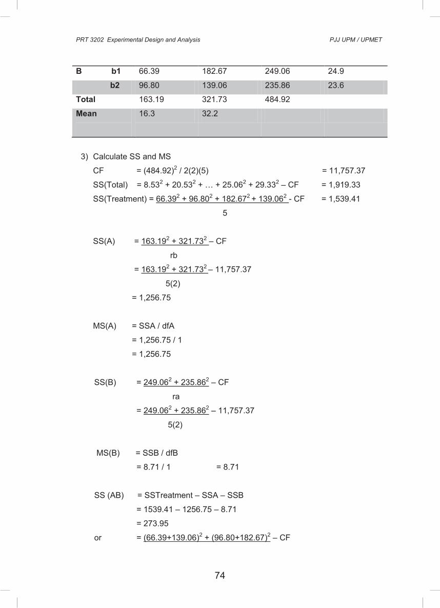
74
PRT 3202 Experimental Design and Analysis PJJ UPM / UPMET
58
B b1 66.39 182.67 249.06 24.9
b2 96.80 139.06 235.86 23.6
Total 163.19 321.73 484.92
Mean
16.3 32.2
3) Calculate SS and MS
CF = (484.92)2 / 2(2)(5) = 11,757.37
SS(Total) = 8.532 + 20.532 + … + 25.062 + 29.332 – CF = 1,919.33
SS(Treatment) = 66.392 + 96.802 + 182.672 + 139.062 - CF = 1,539.41
5
SS(A) = 163.192 + 321.732 – CF
rb
= 163.192 + 321.732 – 11,757.37
5(2)
= 1,256.75
MS(A) = SSA / dfA
= 1,256.75 / 1
= 1,256.75
SS(B) = 249.062 + 235.862 – CF
ra
= 249.062 + 235.862 – 11,757.37
5(2)
MS(B) = SSB / dfB
= 8.71 / 1 = 8.71
SS (AB) = SSTreatment – SSA – SSB
= 1539.41 – 1256.75 – 8.71
= 273.95
or = (66.39+139.06)2 + (96.80+182.67)2 – CF
PRT 3202 Experimental Design and Analysis PJJ UPM / UPMET
59
5(2)
= 12,031.32 – 11,757.37
= 273.95
MS(AB) = SS(AB) / df(AB)
= 273.95 / 1 = 273.95
SS(Error) = SS(total) – SS(treatment)
= 379.92
MS(Error) = SS(error) / df(Error)
= 379.92 / 16 = 23.75
F value, A = MS(A) / MS(Error)
= 1256.75 / 23.75
B = MS(B) / MS(Error)
= 8.71 / 23.75
= 0.4
AB = MS(AB) / MS(Error)
= 273.95 / 23.75
= 11.5
F table: df(n)= 1, df(d)= df(Error)= 16,
p= 0.05 F= 4.49; p= 0.01 F= 4.49
Source of Variation
df SS MS F F table
p= 0.05 p= 0.01
Treatment 3 1539.41
A 1 1256.75 1256.75 52.9** 4.49 8.53
B 1 8.71 8.71 0.4 4.49 8.53
AB 1 273.95 273.95 11.5** 4.49 8.53
Error 16 379.92 23.75
Total 19 1919.33
Conclusion
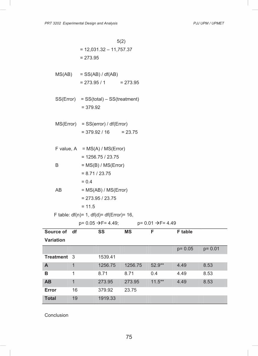
75
PRT 3202 Experimental Design and Analysis PJJ UPM / UPMET
58
B b1 66.39 182.67 249.06 24.9
b2 96.80 139.06 235.86 23.6
Total 163.19 321.73 484.92
Mean
16.3 32.2
3) Calculate SS and MS
CF = (484.92)2 / 2(2)(5) = 11,757.37
SS(Total) = 8.532 + 20.532 + … + 25.062 + 29.332 – CF = 1,919.33
SS(Treatment) = 66.392 + 96.802 + 182.672 + 139.062 - CF = 1,539.41
5
SS(A) = 163.192 + 321.732 – CF
rb
= 163.192 + 321.732 – 11,757.37
5(2)
= 1,256.75
MS(A) = SSA / dfA
= 1,256.75 / 1
= 1,256.75
SS(B) = 249.062 + 235.862 – CF
ra
= 249.062 + 235.862 – 11,757.37
5(2)
MS(B) = SSB / dfB
= 8.71 / 1 = 8.71
SS (AB) = SSTreatment – SSA – SSB
= 1539.41 – 1256.75 – 8.71
= 273.95
or = (66.39+139.06)2 + (96.80+182.67)2 – CF
PRT 3202 Experimental Design and Analysis PJJ UPM / UPMET
59
5(2)
= 12,031.32 – 11,757.37
= 273.95
MS(AB) = SS(AB) / df(AB)
= 273.95 / 1 = 273.95
SS(Error) = SS(total) – SS(treatment)
= 379.92
MS(Error) = SS(error) / df(Error)
= 379.92 / 16 = 23.75
F value, A = MS(A) / MS(Error)
= 1256.75 / 23.75
B = MS(B) / MS(Error)
= 8.71 / 23.75
= 0.4
AB = MS(AB) / MS(Error)
= 273.95 / 23.75
= 11.5
F table: df(n)= 1, df(d)= df(Error)= 16,
p= 0.05 F= 4.49; p= 0.01 F= 4.49
Source of Variation
df SS MS F F table
p= 0.05 p= 0.01
Treatment 3 1539.41
A 1 1256.75 1256.75 52.9** 4.49 8.53
B 1 8.71 8.71 0.4 4.49 8.53
AB 1 273.95 273.95 11.5** 4.49 8.53
Error 16 379.92 23.75
Total 19 1919.33
Conclusion
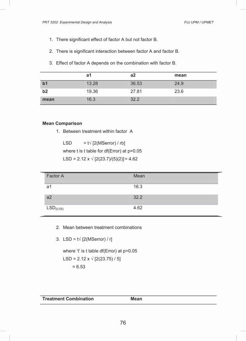
76
PRT 3202 Experimental Design and Analysis PJJ UPM / UPMET
60
1. There significant effect of factor A but not factor B.
2. There is significant interaction between factor A and factor B.
3. Effect of factor A depends on the combination with factor B.
a1 a2 mean
b1 13.28 36.53 24.9
b2 19.36 27.81 23.6
mean 16.3 32.2
Mean Comparison
1. Between treatment within factor A
LSD = t√ [2(MSerror) / rb]
where t is t table for df(Error) at p=0.05
LSD = 2.12 x √ [2(23.7)/(5)(2)] = 4.62
Factor A Mean
a1 16.3
a2 32.2
LSD(0.05) 4.62
2. Mean between treatment combinations
3. LSD = t√ [2(MSerror) / r]
where ‘t’ is t table df(Error) at p=0.05
LSD = 2.12 x √ [2(23.75) / 5]
= 6.53
Treatment Combination Mean
PRT 3202 Experimental Design and Analysis PJJ UPM / UPMET
61
A1b1 13.28
A1b2 19.36
A2b1 36.53
A2b2 27.81
LSD(0.05) 6.53
Laboratory exercise for topic 2 unit 7 will be delivered during week 12 through
LMS or email.
UNIT 8
EXPERIMENT WITH DIFFERENT SIZES OF EXPERIMENTAL UNITS
Introduction
In a certain situation there are experimental designs to overcome the environmental
error.
Objective

77
PRT 3202 Experimental Design and Analysis PJJ UPM / UPMET
60
1. There significant effect of factor A but not factor B.
2. There is significant interaction between factor A and factor B.
3. Effect of factor A depends on the combination with factor B.
a1 a2 mean
b1 13.28 36.53 24.9
b2 19.36 27.81 23.6
mean 16.3 32.2
Mean Comparison
1. Between treatment within factor A
LSD = t√ [2(MSerror) / rb]
where t is t table for df(Error) at p=0.05
LSD = 2.12 x √ [2(23.7)/(5)(2)] = 4.62
Factor A Mean
a1 16.3
a2 32.2
LSD(0.05) 4.62
2. Mean between treatment combinations
3. LSD = t√ [2(MSerror) / r]
where ‘t’ is t table df(Error) at p=0.05
LSD = 2.12 x √ [2(23.75) / 5]
= 6.53
Treatment Combination Mean
PRT 3202 Experimental Design and Analysis PJJ UPM / UPMET
61
A1b1 13.28
A1b2 19.36
A2b1 36.53
A2b2 27.81
LSD(0.05) 6.53
Laboratory exercise for topic 2 unit 7 will be delivered during week 12 through
LMS or email.
UNIT 8
EXPERIMENT WITH DIFFERENT SIZES OF EXPERIMENTAL UNITS
Introduction
In a certain situation there are experimental designs to overcome the environmental
error.
Objective

78
PRT 3202 Experimental Design and Analysis PJJ UPM / UPMET
62
To use different experimental designs with different sizes to reduce environmental
error
Important Content TOPIC 1: SPLIT PLOT DESIGN
For factorial experiment with two factors where the experimental materials do not
allow for the treatment combinations to be arranged in the usual manner.
.. Contains main plot and sub-plot. Sub-plot is arranged within the main plot.
.. First factor is arranged in the main plot and the second factor is arranged in
the sub- plot. Treatments in the main plot and sub-plot are arranged
randomly. Precision of main plot < sub-plot and Error term is separated for
main plot and sub-plot.
PRT 3202 Experimental Design and Analysis PJJ UPM / UPMET
63
N0
Rep 3
Main Plot
N120
N0
Rep 2
N120
N0 Rep 1
N120
Example: Factorial experiment of 2 x 4, with 3 replications.
2 rates of N: 0 kg ha-1 (N0) and 120 kg ha-1 (N120)
4 organic fertilizer: BV, V, F, B
F 20.5
B 25.4
BV 27.6
V 28.4
B 15.2
V 22.3
BV 19.6
F 13.2
BV 18.3
B 15.0
F 13.5
V 22.7
B 24.2
V 24.8
BV 26.7
F 18.0
V 21.0
F 13.8
BV 18.9
B 15.5
B 22.2
F 19.3
V 25.3
BV 25.9
Sub Plot
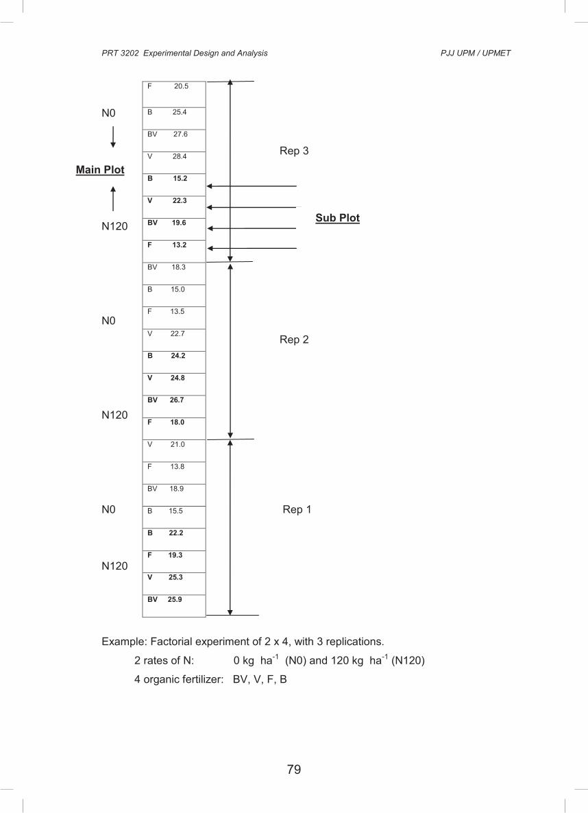
79
PRT 3202 Experimental Design and Analysis PJJ UPM / UPMET
62
To use different experimental designs with different sizes to reduce environmental
error
Important Content TOPIC 1: SPLIT PLOT DESIGN
For factorial experiment with two factors where the experimental materials do not
allow for the treatment combinations to be arranged in the usual manner.
.. Contains main plot and sub-plot. Sub-plot is arranged within the main plot.
.. First factor is arranged in the main plot and the second factor is arranged in
the sub- plot. Treatments in the main plot and sub-plot are arranged
randomly. Precision of main plot < sub-plot and Error term is separated for
main plot and sub-plot.
PRT 3202 Experimental Design and Analysis PJJ UPM / UPMET
63
N0
Rep 3
Main Plot
N120
N0
Rep 2
N120
N0 Rep 1
N120
Example: Factorial experiment of 2 x 4, with 3 replications.
2 rates of N: 0 kg ha-1 (N0) and 120 kg ha-1 (N120)
4 organic fertilizer: BV, V, F, B
F 20.5
B 25.4
BV 27.6
V 28.4
B 15.2
V 22.3
BV 19.6
F 13.2
BV 18.3
B 15.0
F 13.5
V 22.7
B 24.2
V 24.8
BV 26.7
F 18.0
V 21.0
F 13.8
BV 18.9
B 15.5
B 22.2
F 19.3
V 25.3
BV 25.9
Sub Plot
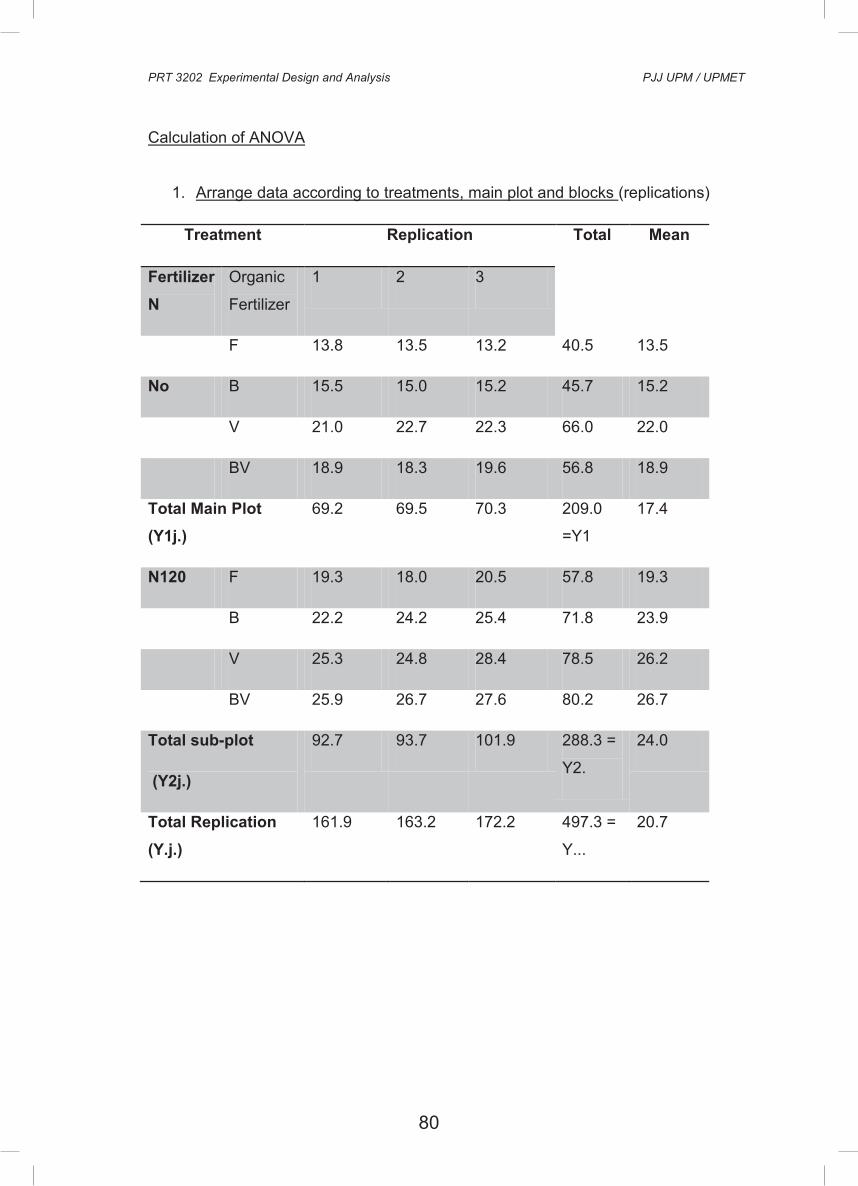
80
PRT 3202 Experimental Design and Analysis PJJ UPM / UPMET
64
Calculation of ANOVA
1. Arrange data according to treatments, main plot and blocks (replications)
Treatment Replication Total Mean
Fertilizer N
Organic
Fertilizer
1 2 3
F 13.8 13.5 13.2 40.5 13.5
No B 15.5 15.0 15.2 45.7 15.2
V 21.0 22.7 22.3 66.0 22.0
BV 18.9 18.3 19.6 56.8 18.9
Total Main Plot (Y1j.)
69.2 69.5 70.3 209.0
=Y1
17.4
N120 F 19.3 18.0 20.5 57.8 19.3
B 22.2 24.2 25.4 71.8 23.9
V 25.3 24.8 28.4 78.5 26.2
BV 25.9 26.7 27.6 80.2 26.7
Total sub-plot
(Y2j.)
92.7 93.7 101.9 288.3 =
Y2.
24.0
Total Replication (Y.j.)
161.9 163.2 172.2 497.3 =
Y...
20.7
PRT 3202 Experimental Design and Analysis PJJ UPM / UPMET
65
2. Arrange data following treatments and sub-plot.
Organic Fertilizer
F B V BV
Total (Y..k) 98.3 117.5 144.5 137.0
Mean (Y..k) 16.3 19.6 24.1 22.8
3. Arrange source of variation and degree of freedom (df)
Source of Variation df
Replication r - 1 = 2
Nitrogen (N) n – 1 = 1
Error for main plot (Error a) (r-1)(n-1) = 2
Organic fertilizer (G) g – 1 = 3
N x G (n - 1)(g – 1) = 3
Error for sub-plot (Error b) (r – 1)(g – 1) + (r – 1)(n – 1)(g – 1)=12
Total ngr-1=23
4. Correction factor (CF)
CF = [Y..]2 / ngr = (497.3)2 / 2(4)(3) = 10,304.47
5. SS and MS
Total SS = Ɛ Yijk2 – CF
= (13.82 + 13.52 +... + 26.72 +27.62) – 10,304.47
= 516.12

81
PRT 3202 Experimental Design and Analysis PJJ UPM / UPMET
64
Calculation of ANOVA
1. Arrange data according to treatments, main plot and blocks (replications)
Treatment Replication Total Mean
Fertilizer N
Organic
Fertilizer
1 2 3
F 13.8 13.5 13.2 40.5 13.5
No B 15.5 15.0 15.2 45.7 15.2
V 21.0 22.7 22.3 66.0 22.0
BV 18.9 18.3 19.6 56.8 18.9
Total Main Plot (Y1j.)
69.2 69.5 70.3 209.0
=Y1
17.4
N120 F 19.3 18.0 20.5 57.8 19.3
B 22.2 24.2 25.4 71.8 23.9
V 25.3 24.8 28.4 78.5 26.2
BV 25.9 26.7 27.6 80.2 26.7
Total sub-plot
(Y2j.)
92.7 93.7 101.9 288.3 =
Y2.
24.0
Total Replication (Y.j.)
161.9 163.2 172.2 497.3 =
Y...
20.7
PRT 3202 Experimental Design and Analysis PJJ UPM / UPMET
65
2. Arrange data following treatments and sub-plot.
Organic Fertilizer
F B V BV
Total (Y..k) 98.3 117.5 144.5 137.0
Mean (Y..k) 16.3 19.6 24.1 22.8
3. Arrange source of variation and degree of freedom (df)
Source of Variation df
Replication r - 1 = 2
Nitrogen (N) n – 1 = 1
Error for main plot (Error a) (r-1)(n-1) = 2
Organic fertilizer (G) g – 1 = 3
N x G (n - 1)(g – 1) = 3
Error for sub-plot (Error b) (r – 1)(g – 1) + (r – 1)(n – 1)(g – 1)=12
Total ngr-1=23
4. Correction factor (CF)
CF = [Y..]2 / ngr = (497.3)2 / 2(4)(3) = 10,304.47
5. SS and MS
Total SS = Ɛ Yijk2 – CF
= (13.82 + 13.52 +... + 26.72 +27.62) – 10,304.47
= 516.12
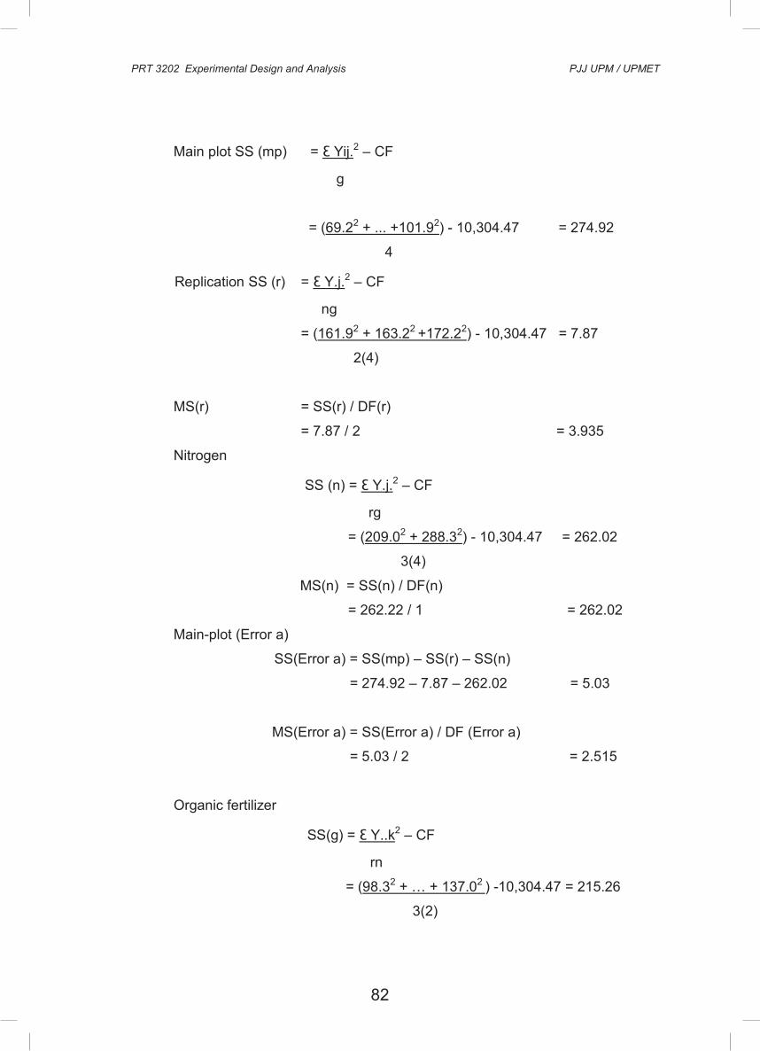
82
PRT 3202 Experimental Design and Analysis PJJ UPM / UPMET
66
Main plot SS (mp) = Ɛ Yij.2 – CF
g
= (69.22 + ... +101.92) - 10,304.47 = 274.92
4
Replication SS (r) = Ɛ Y.j.2 – CF
ng
= (161.92 + 163.22 +172.22) - 10,304.47 = 7.87
2(4)
MS(r) = SS(r) / DF(r)
= 7.87 / 2 = 3.935
Nitrogen
SS (n) = Ɛ Y.j.2 – CF
rg
= (209.02 + 288.32) - 10,304.47 = 262.02
3(4)
MS(n) = SS(n) / DF(n)
= 262.22 / 1 = 262.02
Main-plot (Error a)
SS(Error a) = SS(mp) – SS(r) – SS(n)
= 274.92 – 7.87 – 262.02 = 5.03
MS(Error a) = SS(Error a) / DF (Error a)
= 5.03 / 2 = 2.515
Organic fertilizer
SS(g) = Ɛ Y..k2 – CF
rn
= (98.32 + … + 137.02 ) -10,304.47 = 215.26
3(2)
PRT 3202 Experimental Design and Analysis PJJ UPM / UPMET
67
MS(g) = SS(g) / DF(g)
= 215.26 / 3 = 71.753
Nitrogen x Organic fertilizer
SS(nxg) = Ɛ Yi..k2 – CF – SS(n) – SS(g)
r
= (40.52 + … + 80.22) - 10,304.47 – 262.02 – 215.26 = 18.70
3
MS(nxg) = SS(nxg) / DF(nxg)
= 18.70 / 3 = 6.233
Error sub-plot (Error b)
SS(Error b) = SS(t) – SS(mp) – SS(g) – SS(nxg)
= 516.12 – 274.92 – 215.26 -18.70 = 7.24
MS(Error b) = SS(Error b) / DF(Error b)
= 7.24 / 12 = 0.603
6. F value
Nitrogen
Effect of nitrogen is tested using Error of main plot (Error a)
F(n) = MS(n) / MS(Error a)
= 262.02 / 2.515
= 104.18
F(table): DF(n)= 1, DF(Error a)= 2, p= 0.05 F= 18.51
Organic fertilizer and interaction between nitrogen x organic fertilizer,
use error of sub-plot (Error b),
F(g) = MS(g) / MS(Error b)
= 71.753 / 0.603 = 118.99
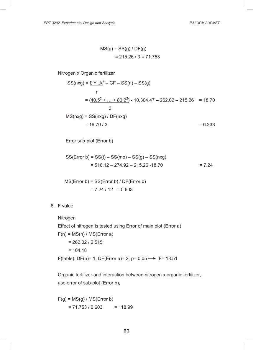
83
PRT 3202 Experimental Design and Analysis PJJ UPM / UPMET
66
Main plot SS (mp) = Ɛ Yij.2 – CF
g
= (69.22 + ... +101.92) - 10,304.47 = 274.92
4
Replication SS (r) = Ɛ Y.j.2 – CF
ng
= (161.92 + 163.22 +172.22) - 10,304.47 = 7.87
2(4)
MS(r) = SS(r) / DF(r)
= 7.87 / 2 = 3.935
Nitrogen
SS (n) = Ɛ Y.j.2 – CF
rg
= (209.02 + 288.32) - 10,304.47 = 262.02
3(4)
MS(n) = SS(n) / DF(n)
= 262.22 / 1 = 262.02
Main-plot (Error a)
SS(Error a) = SS(mp) – SS(r) – SS(n)
= 274.92 – 7.87 – 262.02 = 5.03
MS(Error a) = SS(Error a) / DF (Error a)
= 5.03 / 2 = 2.515
Organic fertilizer
SS(g) = Ɛ Y..k2 – CF
rn
= (98.32 + … + 137.02 ) -10,304.47 = 215.26
3(2)
PRT 3202 Experimental Design and Analysis PJJ UPM / UPMET
67
MS(g) = SS(g) / DF(g)
= 215.26 / 3 = 71.753
Nitrogen x Organic fertilizer
SS(nxg) = Ɛ Yi..k2 – CF – SS(n) – SS(g)
r
= (40.52 + … + 80.22) - 10,304.47 – 262.02 – 215.26 = 18.70
3
MS(nxg) = SS(nxg) / DF(nxg)
= 18.70 / 3 = 6.233
Error sub-plot (Error b)
SS(Error b) = SS(t) – SS(mp) – SS(g) – SS(nxg)
= 516.12 – 274.92 – 215.26 -18.70 = 7.24
MS(Error b) = SS(Error b) / DF(Error b)
= 7.24 / 12 = 0.603
6. F value
Nitrogen
Effect of nitrogen is tested using Error of main plot (Error a)
F(n) = MS(n) / MS(Error a)
= 262.02 / 2.515
= 104.18
F(table): DF(n)= 1, DF(Error a)= 2, p= 0.05 F= 18.51
Organic fertilizer and interaction between nitrogen x organic fertilizer,
use error of sub-plot (Error b),
F(g) = MS(g) / MS(Error b)
= 71.753 / 0.603 = 118.99
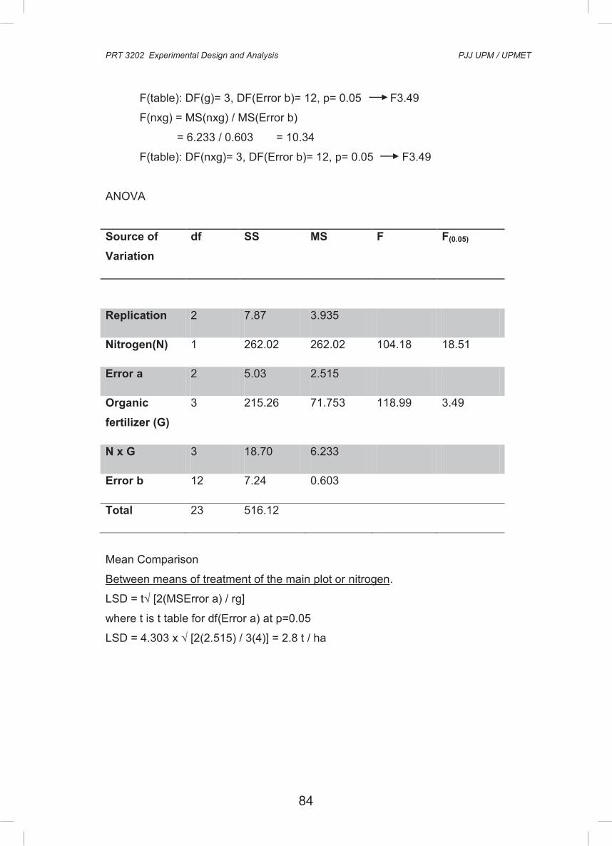
84
PRT 3202 Experimental Design and Analysis PJJ UPM / UPMET
68
F(table): DF(g)= 3, DF(Error b)= 12, p= 0.05 F3.49
F(nxg) = MS(nxg) / MS(Error b)
= 6.233 / 0.603 = 10.34
F(table): DF(nxg)= 3, DF(Error b)= 12, p= 0.05 F3.49
ANOVA
Source of Variation
df SS MS F F(0.05)
Replication 2 7.87 3.935
Nitrogen(N) 1 262.02 262.02 104.18 18.51
Error a 2 5.03 2.515
Organic fertilizer (G)
3 215.26 71.753 118.99 3.49
N x G 3 18.70 6.233
Error b 12 7.24 0.603
Total 23 516.12
Mean Comparison
Between means of treatment of the main plot or nitrogen.
LSD = t√ [2(MSError a) / rg]
where t is t table for df(Error a) at p=0.05
LSD = 4.303 x √ [2(2.515) / 3(4)] = 2.8 t / ha
PRT 3202 Experimental Design and Analysis PJJ UPM / UPMET
69
N (kg ha-1) Yield (t ha-1)
0 17.4
120 24.0
LSD 0.05 2.8
Between treatments of the sub-plot or organic fertilizer.
LSD = t√ [2(MSError b) / rn]
where t is t table for df(Error b) at p=0.05
LSD = 2.179 x √ [2(0.603) / 3(2)]
= 1.0 t ha-1
Organic fertilizer Yield (t ha-1)
F 16.4
B 19.6
BV 22.8
V 24.1
LSD0.05 1.0
Conclusion 1. There is significant effect of nitrogen on the yield at p = 0.05
Applying N at the rate of 120 kg ha-1 obtained higher yield than at 0.
2. There is significant effect of organic fertilizer on the yield. Organic fertilizer V the highest yield followed by BV, B and F.
Laboratory exercise for topic 1 unit 8 will be delivered during week 13 through
LMS or email.

85
PRT 3202 Experimental Design and Analysis PJJ UPM / UPMET
68
F(table): DF(g)= 3, DF(Error b)= 12, p= 0.05 F3.49
F(nxg) = MS(nxg) / MS(Error b)
= 6.233 / 0.603 = 10.34
F(table): DF(nxg)= 3, DF(Error b)= 12, p= 0.05 F3.49
ANOVA
Source of Variation
df SS MS F F(0.05)
Replication 2 7.87 3.935
Nitrogen(N) 1 262.02 262.02 104.18 18.51
Error a 2 5.03 2.515
Organic fertilizer (G)
3 215.26 71.753 118.99 3.49
N x G 3 18.70 6.233
Error b 12 7.24 0.603
Total 23 516.12
Mean Comparison
Between means of treatment of the main plot or nitrogen.
LSD = t√ [2(MSError a) / rg]
where t is t table for df(Error a) at p=0.05
LSD = 4.303 x √ [2(2.515) / 3(4)] = 2.8 t / ha
PRT 3202 Experimental Design and Analysis PJJ UPM / UPMET
69
N (kg ha-1) Yield (t ha-1)
0 17.4
120 24.0
LSD 0.05 2.8
Between treatments of the sub-plot or organic fertilizer.
LSD = t√ [2(MSError b) / rn]
where t is t table for df(Error b) at p=0.05
LSD = 2.179 x √ [2(0.603) / 3(2)]
= 1.0 t ha-1
Organic fertilizer Yield (t ha-1)
F 16.4
B 19.6
BV 22.8
V 24.1
LSD0.05 1.0
Conclusion 1. There is significant effect of nitrogen on the yield at p = 0.05
Applying N at the rate of 120 kg ha-1 obtained higher yield than at 0.
2. There is significant effect of organic fertilizer on the yield. Organic fertilizer V the highest yield followed by BV, B and F.
Laboratory exercise for topic 1 unit 8 will be delivered during week 13 through
LMS or email.
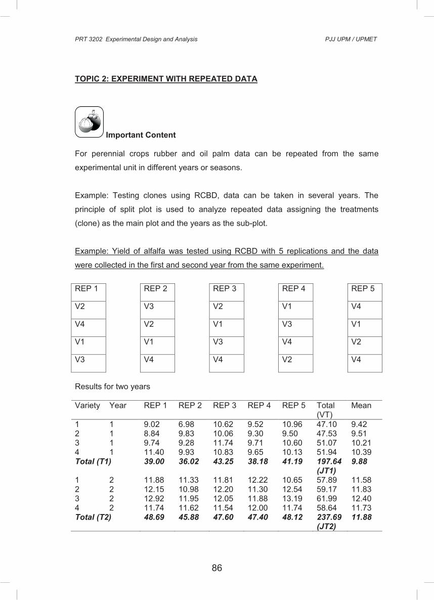
86
PRT 3202 Experimental Design and Analysis PJJ UPM / UPMET
70
TOPIC 2: EXPERIMENT WITH REPEATED DATA
Important Content For perennial crops rubber and oil palm data can be repeated from the same
experimental unit in different years or seasons.
Example: Testing clones using RCBD, data can be taken in several years. The
principle of split plot is used to analyze repeated data assigning the treatments
(clone) as the main plot and the years as the sub-plot.
Example: Yield of alfalfa was tested using RCBD with 5 replications and the data
were collected in the first and second year from the same experiment.
REP 1 REP 2 REP 3 REP 4 REP 5
V2 V3 V2 V1 V4
V4 V2 V1 V3 V1
V1 V1 V3 V4 V2
V3 V4 V4 V2 V4
Results for two years Variety Year REP 1 REP 2 REP 3 REP 4 REP 5 Total
(VT) Mean
1 1 9.02 6.98 10.62 9.52 10.96 47.10 9.42 2 1 8.84 9.83 10.06 9.30 9.50 47.53 9.51 3 1 9.74 9.28 11.74 9.71 10.60 51.07 10.21 4 1 11.40 9.93 10.83 9.65 10.13 51.94 10.39 Total (T1) 39.00 36.02 43.25 38.18 41.19 197.64
(JT1) 9.88
1 2 11.88 11.33 11.81 12.22 10.65 57.89 11.58 2 2 12.15 10.98 12.20 11.30 12.54 59.17 11.83 3 2 12.92 11.95 12.05 11.88 13.19 61.99 12.40 4 2 11.74 11.62 11.54 12.00 11.74 58.64 11.73 Total (T2) 48.69 45.88 47.60 47.40 48.12 237.69
(JT2) 11.88
PRT 3202 Experimental Design and Analysis PJJ UPM / UPMET
71
Table of Variety x Replication
Variety REP 1 REP 2 REP 3 REP 4 REP 5 Total (V)
Mean
1 20.90 18.31 22.43 21.74 21.64 105.02 10.50 2 20.99 20.79 22.26 20.60 22.04 106.68 10.67 3 22.66 21.23 23.79 21.59 23.79 113.06 11.31 4 23.14 21.55 22.37 21.65 21.87 110.58 11.06 Total (R) 87.69 81.88 90.85 85.58 89.34 435.34 (JK) Hypothesis: No significant difference between the means of variety.
No significant difference between means of years.
No significant interaction between variety and year.
ANOVA of yield for two years
Source of Variation
df SS MS F F table
5% 1% Replication, R
4 6.13 1.53 4.78 3.26 5.41
Variety, V 3 4.01 1.34 4.18 3.49 5.95 Error (a), VR 12 3.89 0.32 Year , Y 1 39.89 39.89 55.40 4.49 8.53 V x Y 3 1.51 0.50 0.69 3.24 5.29 Error (b), RY+R(VY)
16 11.54 0.72
Total 39 66.95
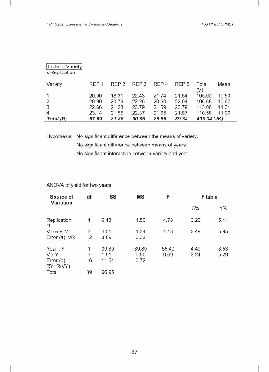
87
PRT 3202 Experimental Design and Analysis PJJ UPM / UPMET
70
TOPIC 2: EXPERIMENT WITH REPEATED DATA
Important Content For perennial crops rubber and oil palm data can be repeated from the same
experimental unit in different years or seasons.
Example: Testing clones using RCBD, data can be taken in several years. The
principle of split plot is used to analyze repeated data assigning the treatments
(clone) as the main plot and the years as the sub-plot.
Example: Yield of alfalfa was tested using RCBD with 5 replications and the data
were collected in the first and second year from the same experiment.
REP 1 REP 2 REP 3 REP 4 REP 5
V2 V3 V2 V1 V4
V4 V2 V1 V3 V1
V1 V1 V3 V4 V2
V3 V4 V4 V2 V4
Results for two years Variety Year REP 1 REP 2 REP 3 REP 4 REP 5 Total
(VT) Mean
1 1 9.02 6.98 10.62 9.52 10.96 47.10 9.42 2 1 8.84 9.83 10.06 9.30 9.50 47.53 9.51 3 1 9.74 9.28 11.74 9.71 10.60 51.07 10.21 4 1 11.40 9.93 10.83 9.65 10.13 51.94 10.39 Total (T1) 39.00 36.02 43.25 38.18 41.19 197.64
(JT1) 9.88
1 2 11.88 11.33 11.81 12.22 10.65 57.89 11.58 2 2 12.15 10.98 12.20 11.30 12.54 59.17 11.83 3 2 12.92 11.95 12.05 11.88 13.19 61.99 12.40 4 2 11.74 11.62 11.54 12.00 11.74 58.64 11.73 Total (T2) 48.69 45.88 47.60 47.40 48.12 237.69
(JT2) 11.88
PRT 3202 Experimental Design and Analysis PJJ UPM / UPMET
71
Table of Variety x Replication
Variety REP 1 REP 2 REP 3 REP 4 REP 5 Total (V)
Mean
1 20.90 18.31 22.43 21.74 21.64 105.02 10.50 2 20.99 20.79 22.26 20.60 22.04 106.68 10.67 3 22.66 21.23 23.79 21.59 23.79 113.06 11.31 4 23.14 21.55 22.37 21.65 21.87 110.58 11.06 Total (R) 87.69 81.88 90.85 85.58 89.34 435.34 (JK) Hypothesis: No significant difference between the means of variety.
No significant difference between means of years.
No significant interaction between variety and year.
ANOVA of yield for two years
Source of Variation
df SS MS F F table
5% 1% Replication, R
4 6.13 1.53 4.78 3.26 5.41
Variety, V 3 4.01 1.34 4.18 3.49 5.95 Error (a), VR 12 3.89 0.32 Year , Y 1 39.89 39.89 55.40 4.49 8.53 V x Y 3 1.51 0.50 0.69 3.24 5.29 Error (b), RY+R(VY)
16 11.54 0.72
Total 39 66.95

88
PRT 3202 Experimental Design and Analysis PJJ UPM / UPMET
72
Calculation 1. df
Total = RVY-1 = (5)(4)(2) – 1 = 39
Replication = R-1 = 5-1 = 4
Variety = V-1 = 4-1 = 3
Error (a) = (R-1)(V-1) = (5-1)(4-1) = 12
Year = Y-1 = 2-1 = 1
Y x V = (Y-1) (V-1) = (2-1)(4-1) = 3
Error (b) = (R-1) (Y-1) + (R-1)(V-1)(Y-1)
= (5-1) (2-1) + (5-1)(4-1)(2-1) = 16
2. CF = (JK)2/ rat = (435.31)2 / (5)(4)(2) = 4738.02 3. SS Total = SSJ = Ʃ(Y)2 – CF
= (9.022+...+11.742) – 4738.02 = 66.95
4. SS Replication = SSR = [Ʃ(R) 2 / vy] – CF = [(87.692+ ... + 89.312) / 4(2)] – 4738.02 = 6.13
5. SSVariety = SSV = [Ʃ(V) 2 / ry] – CF = [(104.992+ ... + 110.582) / 5(2)] – 4738.02 = 4.01
6. SSError (a) = SSE (a) = [Ʃ(VR) 2 / y] – CF – SSR – SSV = [20.902+ ... + 21.872) / 2] – 4738.02 – 6.13 – 4.01 = 3.87
7. SSYear = SST = [Ʃ(Y) 2 / rv] – CF
= [(197.642+ 237.692) / 5(4)] – 4738.02 = 39.89
8. SSVariety x Year = SSVY = [Ʃ(VY) 2 / r] – CF – SSV – SSY = [(47.102+ ... +58.642) / 5] – 4738.02 – 4.01 – 39.89 = 1.51
PRT 3202 Experimental Design and Analysis PJJ UPM / UPMET
73
9. SSError (b) = SSE (b) = SSJ – SSR – SSV – SSE(a) – SSY – SSVY
= 66.95 – 6.13 – 4.01 – 3.87 – 39.89 – 1.51 = 11. 54
10. Mean Square MSR = SSR/ DFR = 6.13 / 4 = 1.53 MSV = SSV/ DFV = 4.01 / 3 = 1.34 MST = SST/ DFT = 39.89 / 1 = 39.89 MSVT = SSVT/ DFVT = 1.51 / 3 = 0.50
11. F value Replication F = MSR / MSE (a) = 1.53 / 0.32 = 4.78 Variety F = MSV / MSE (a)
= 1.34 / 0.32 = 4.18
Year F = MSY / MSE (b)
= 39.89 / 0.72 = 55.40 Variety x Year F = MSVY/ MSE (b)
= 0.50 / 0.72 = 0.69

89
PRT 3202 Experimental Design and Analysis PJJ UPM / UPMET
72
Calculation 1. df
Total = RVY-1 = (5)(4)(2) – 1 = 39
Replication = R-1 = 5-1 = 4
Variety = V-1 = 4-1 = 3
Error (a) = (R-1)(V-1) = (5-1)(4-1) = 12
Year = Y-1 = 2-1 = 1
Y x V = (Y-1) (V-1) = (2-1)(4-1) = 3
Error (b) = (R-1) (Y-1) + (R-1)(V-1)(Y-1)
= (5-1) (2-1) + (5-1)(4-1)(2-1) = 16
2. CF = (JK)2/ rat = (435.31)2 / (5)(4)(2) = 4738.02 3. SS Total = SSJ = Ʃ(Y)2 – CF
= (9.022+...+11.742) – 4738.02 = 66.95
4. SS Replication = SSR = [Ʃ(R) 2 / vy] – CF = [(87.692+ ... + 89.312) / 4(2)] – 4738.02 = 6.13
5. SSVariety = SSV = [Ʃ(V) 2 / ry] – CF = [(104.992+ ... + 110.582) / 5(2)] – 4738.02 = 4.01
6. SSError (a) = SSE (a) = [Ʃ(VR) 2 / y] – CF – SSR – SSV = [20.902+ ... + 21.872) / 2] – 4738.02 – 6.13 – 4.01 = 3.87
7. SSYear = SST = [Ʃ(Y) 2 / rv] – CF
= [(197.642+ 237.692) / 5(4)] – 4738.02 = 39.89
8. SSVariety x Year = SSVY = [Ʃ(VY) 2 / r] – CF – SSV – SSY = [(47.102+ ... +58.642) / 5] – 4738.02 – 4.01 – 39.89 = 1.51
PRT 3202 Experimental Design and Analysis PJJ UPM / UPMET
73
9. SSError (b) = SSE (b) = SSJ – SSR – SSV – SSE(a) – SSY – SSVY
= 66.95 – 6.13 – 4.01 – 3.87 – 39.89 – 1.51 = 11. 54
10. Mean Square MSR = SSR/ DFR = 6.13 / 4 = 1.53 MSV = SSV/ DFV = 4.01 / 3 = 1.34 MST = SST/ DFT = 39.89 / 1 = 39.89 MSVT = SSVT/ DFVT = 1.51 / 3 = 0.50
11. F value Replication F = MSR / MSE (a) = 1.53 / 0.32 = 4.78 Variety F = MSV / MSE (a)
= 1.34 / 0.32 = 4.18
Year F = MSY / MSE (b)
= 39.89 / 0.72 = 55.40 Variety x Year F = MSVY/ MSE (b)
= 0.50 / 0.72 = 0.69

90
PRT 3202 Experimental Design and Analysis PJJ UPM / UPMET
74
Table of ANOVA
Source of Variation
df SS MS F F Table
5% 1% Replication,R 4 6.13 1.53 4.78 3.26 5.41 Variety, V 3 4.01 1.34 4.18 3.49 5.95 Error (a), VR 12 3.89 0.32 Year, Y 1 39.89 39.89 55.40 4.49 8.53 V x T 3 1.51 0.50 0.69 3.24 5.29 Error (b), RY+R(VY)
16 11.54 0.72
Total 39 66.95
Conclusion
1. There is a significant difference for means of years and varieties.
2. There is no interaction between year and variety.
Mean Comparison (LSD) Comparison between means of variety
LSD = t [√ (2MSE (a) / ry)]
Where t is value of t table at p = 0.05, dfe (a) = 12 t = 2.179
LSD = 2.179 x √ [2(0.32) / 5(2)] = 0.55
Variety Yield (t ha-1)
1 10.50
2 10.67
3 11.31
4 11.06
LSD0.05 0.55
PRT 3202 Experimental Design and Analysis PJJ UPM / UPMET
75
Comparison between means of years
LSD = t [√ (2MSE (b) / rv)]
LSD = 2.120 x √ [2(0.72) / 5(4)] = 0.57
Variety Yield (t ha-1)
1 9.88
2 11.88
LSD0.05 0.57
Laboratory exercise for topic 2 unit 8 will be delivered during week 14 through
LMS or email.

91
PRT 3202 Experimental Design and Analysis PJJ UPM / UPMET
74
Table of ANOVA
Source of Variation
df SS MS F F Table
5% 1% Replication,R 4 6.13 1.53 4.78 3.26 5.41 Variety, V 3 4.01 1.34 4.18 3.49 5.95 Error (a), VR 12 3.89 0.32 Year, Y 1 39.89 39.89 55.40 4.49 8.53 V x T 3 1.51 0.50 0.69 3.24 5.29 Error (b), RY+R(VY)
16 11.54 0.72
Total 39 66.95
Conclusion
1. There is a significant difference for means of years and varieties.
2. There is no interaction between year and variety.
Mean Comparison (LSD) Comparison between means of variety
LSD = t [√ (2MSE (a) / ry)]
Where t is value of t table at p = 0.05, dfe (a) = 12 t = 2.179
LSD = 2.179 x √ [2(0.32) / 5(2)] = 0.55
Variety Yield (t ha-1)
1 10.50
2 10.67
3 11.31
4 11.06
LSD0.05 0.55
PRT 3202 Experimental Design and Analysis PJJ UPM / UPMET
75
Comparison between means of years
LSD = t [√ (2MSE (b) / rv)]
LSD = 2.120 x √ [2(0.72) / 5(4)] = 0.57
Variety Yield (t ha-1)
1 9.88
2 11.88
LSD0.05 0.57
Laboratory exercise for topic 2 unit 8 will be delivered during week 14 through
LMS or email.