lampiran a hasil uji standarisasirepository.wima.ac.id/533/7/lampiran.pdf · hasil perhitungan...
TRANSCRIPT
73
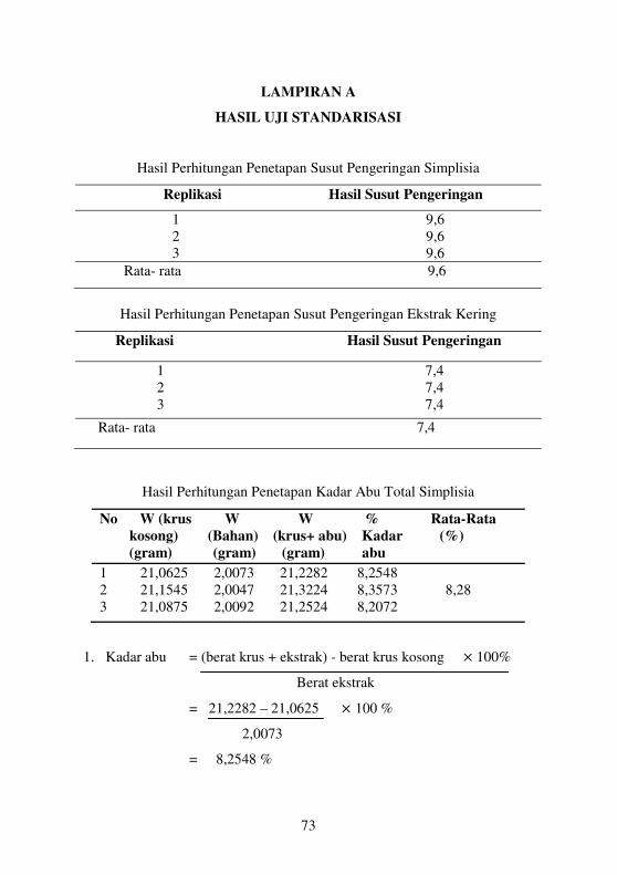
LAMPIRAN A
HASIL UJI STANDARISASI
Hasil Perhitungan Penetapan Susut Pengeringan Simplisia
Replikasi Hasil Susut Pengeringan
1 9,6 2 9,6 3 9,6
Rata- rata 9,6
Hasil Perhitungan Penetapan Susut Pengeringan Ekstrak Kering
Replikasi Hasil Susut Pengeringan
1 7,4 2 7,4 3 7,4
Rata- rata 7,4
Hasil Perhitungan Penetapan Kadar Abu Total Simplisia
No W (krus W W % Rata-Rata
kosong) (Bahan) (krus+ abu) Kadar (%)
(gram) (gram) (gram) abu
1 21,0625 2,0073 21,2282 8,2548 2 21,1545 2,0047 21,3224 8,3573 8,28 3 21,0875 2,0092 21,2524 8,2072
1. Kadar abu = (berat krus + ekstrak) - berat krus kosong F 100%
Berat ekstrak
= 21,2282 – 21,0625 F 100 %
2,0073
= 8,2548 %
74
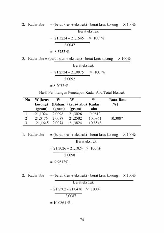
2. Kadar abu = (berat krus + ekstrak) - berat krus kosong F 100%
Berat ekstrak
= 21,3224 – 21,1545 F 100 %
2,0047
= 8,3753 %
3. Kadar abu = (berat krus + ekstrak) - berat krus kosong F 100%
Berat ekstrak
= 21,2524 – 21,0875 F 100 %
2.0092
= 8,2072 %
Hasil Perhitungan Penetapan Kadar Abu Total Ekstrak
No W (krus W W % Rata-Rata
kosong) (Bahan) (krus+ abu) Kadar (%)
(gram) (gram) (gram) abu
1 21,1024 2,0098 21,3026 9,9612 2 21,0476 2,0087 21,2502 10,0861 10,3007 3 21,1645 2,0074 21,3824 10,8548
1. Kadar abu = (berat krus + ekstrak) - berat krus kosong F 100%
Berat ekstrak
= 21,3026 – 21,1024 F 100 %
2,0098
= 9,9612%.
2. Kadar abu = (berat krus + ekstrak) - berat krus kosong F 100%
Berat ekstrak
= 21,2502 - 21,0476 F 100%
2,0087
= 10,0861 %.
75
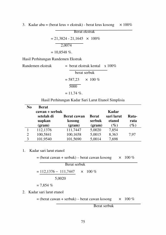
3. Kadar abu = (berat krus + ekstrak) - berat krus kosong F 100%
Berat ekstrak
= 21,3824 - 21,1645 F 100%
2,0074
= 10,8548 %.
Hasil Perhitungan Randemen Ekstrak
Randemen ekstrak = berat ekstrak kental x 100%
berat serbuk
= 587,23 F 100 %
5000
= 11,74 %.
Hasil Perhitungan Kadar Sari Larut Etanol Simplisia
No Berat
cawan + serbuk Kadar
setelah di Berat cawan Berat sari larut Rata-
uapkan kosong serbuk etanol rata
(gram) (gram) (gram) (%) (%)
1 112,1376 111,7447 5,0020 7,854 2 100,5841 100,1658 5,0015 8,363 7,97 3 101,9540 101,5690 5,0014 7,698
1. Kadar sari larut etanol
= (berat cawan + serbuk) – berat cawan kosong F 100 %
Berat serbuk
= 112,1376 − 111,7447 F 100 %
5,0020
= 7,854 %
2. Kadar sari larut etanol
= (berat cawan + serbuk) – berat cawan kosong F 100 %
Berat serbuk

76
= 100,5841 – 100,1658 F 100 %
5,0015
= 8,363 %
3. Kadar sari larut etanol
= (berat cawan + serbuk) – berat cawan kosong F 100 %
Berat serbuk
= 101,9540 − 101,5690 F 100 %
5,0014
= 7,698 %
Hasil Perhitungan Kadar Sari Larut Air Simplisia
No Berat
cawan + serbuk Kadar
setelah di Berat cawan Berat sari larut Rata-
uapkan kosong serbuk air rata
(gram) (gram) (gram) (%) (%)
1 61,8367 61,2286 5,0027 12,1554 2 63,1146 62,5570 5,0019 11,1477 11,64 % 3 61,7951 61,2134 5,0020 11,6293
Hasil Perhitungan Kadar Sari Larut Etanol Ekstrak
No Berat
cawan + serbuk Kadar
setelah di Berat cawan Berat sari larut Rata-
uapkan kosong serbuk etanol rata
(gram) (gram) (gram) (%) (%)
1 61,7395 61,2522 5,0008 9,7444 2 63,0462 62,5981 5,0012 8,9598 9,0974 3 42,6714 42,2164 5,0014 9,0974
77
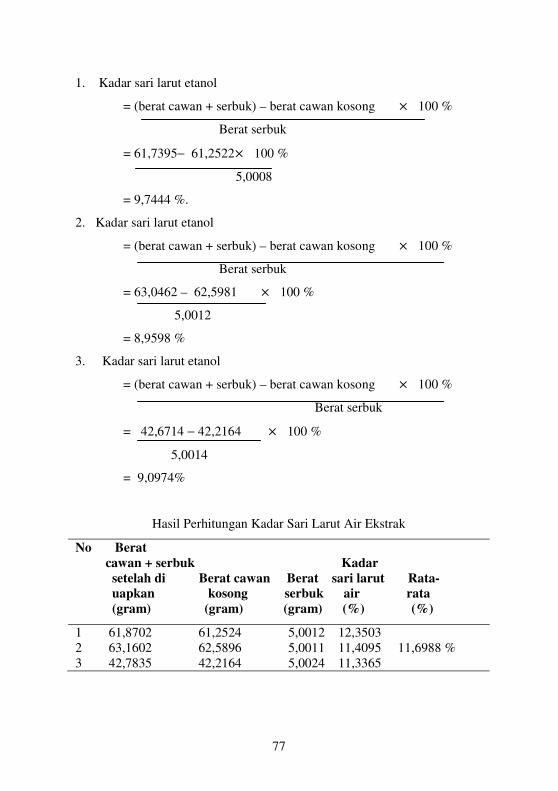
1. Kadar sari larut etanol
= (berat cawan + serbuk) – berat cawan kosong F 100 %
Berat serbuk
= 61,7395− 61,2522F 100 %
5,0008
= 9,7444 %.
2. Kadar sari larut etanol
= (berat cawan + serbuk) – berat cawan kosong F 100 %
Berat serbuk
= 63,0462 – 62,5981 F 100 %
5,0012
= 8,9598 %
3. Kadar sari larut etanol
= (berat cawan + serbuk) – berat cawan kosong F 100 %
Berat serbuk
= 42,6714 − 42,2164 F 100 %
5,0014
= 9,0974%
Hasil Perhitungan Kadar Sari Larut Air Ekstrak
No Berat
cawan + serbuk Kadar
setelah di Berat cawan Berat sari larut Rata-
uapkan kosong serbuk air rata
(gram) (gram) (gram) (%) (%)
1 61,8702 61,2524 5,0012 12,3503 2 63,1602 62,5896 5,0011 11,4095 11,6988 % 3 42,7835 42,2164 5,0024 11,3365
78
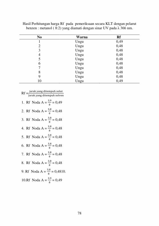
Hasil Perhitungan harga Rf pada pemeriksaan secara KLT dengan pelarut benzen : metanol ( 8:2) yang diamati dengan sinar UV pada λ 366 nm.
No Warna Rf
1 2 3 4 5 6 7 8 9
10
Ungu Ungu Ungu Ungu Ungu Ungu Ungu Ungu Ungu Ungu
0,49 0,48 0,48 0,48 0,48 0,48 0,48 0,48 0,48 0,49
Rf =!"#"$ %"&' ()*+,-./ 012.*
3"#"$ %"&' ()*+,-./ 0124+&
1. Rf Noda A = �,G
� = 0,49
2. Rf Noda A = �,�
� = 0,48
3. Rf Noda A = �,�
� = 0,48
4. Rf Noda A = �,�
� = 0,48
5. Rf Noda A = �,�
� = 0,48
6. Rf Noda A = �,�
� = 0,48
7. Rf Noda A = �,�
� = 0,48
8. Rf Noda A = �,�
� = 0,48
9. Rf Noda A = �,�
� = 0,4810.
10.Rf Noda A = �,G
� = 0,49
79
Isolasi Senyawa Karantin
Ditimbang sejumlah 150 gram serbuk buah pare dan dicampur
dengan pelarut petroleum eter secukupnya hingga rata dan cukup basah
untuk menghilangkan lemaknya, selanjutnya massa tersebut dipindahkan ke
dalam perkolator. Etanol 96% dituang lagi hingga cairan penyari berada 2-
3 cm di atas massa serbuk. Selanjutnya bagian atas perkolator ditutup
dengan cairan penyari yang berada di dalam perkolator didiamkan selama
24 jam. Setelah itu, kran perkolator ditutup. Perkolat ditampung dengan
kecepatan sekitar 1 ml/menit dan secara bertahap ditambahkan etanol 96%
secukupnya dengan kecepatan sama hingga perkolat yang ditampuh sudah
tidak berwarna pekat. Ekstrak cair yang diperoleh selanjutnya dikeringkan
engan menggunakan vacuum evaporator sampai diperoleh ekstrak kental.
Ekstrak kental dibasakan dengan larutan KOH hingga diperoleh PH=10.
Ekstrak kental tersebut didiamkan selama dua hari, diencerkan dengan
aquades, diekstraksi kembali menggunakan eter.
Fase eter ditampung dan dicuci berturut- turut dengan aquadest,
HCl 5%,dilanjutkan dengan aquaest lagi. Jika masih terdapat sisa aquadest
dalam fase eter ditambahkan natrium sulfat anhidrat, kemudian diuapkan
higga kering. Residu direkristalisasi dengan menggunakan etanol 96%.
Kristal karantin yang diperoleh dengan menetapkan harga Rf, indeks bias,
dan titik lebur ( Darsono, FL., 2006).
80
LAMPIRAN B
HASIL UJI KESERAGAMAN BOBOT TABLET EKSTRAK DAUN
PARE
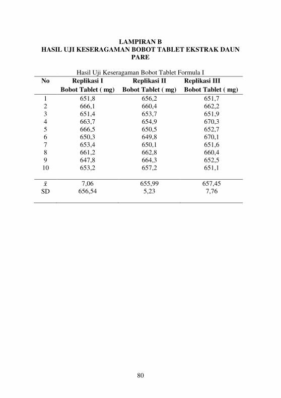
Hasil Uji Keseragaman Bobot Tablet Formula I
No Replikasi I
Bobot Tablet ( mg)
Replikasi II
Bobot Tablet ( mg)
Replikasi III
Bobot Tablet ( mg)
1 2 3 4 5 6 7 8 9 10
651,8 666,1 651,4 663,7 666,5 650,3 653,4 661,2 647,8 653,2
656,2 660,4 653,7 654,9 650,5 649,8 650,1 662,8 664,3 657,2
651,7 662,2 651,9 670,3 652,7 670,1 651,6 660,4 652,5 651,1
HI SD
7,06 656,54
655,99 5,23
657,45 7,76
81
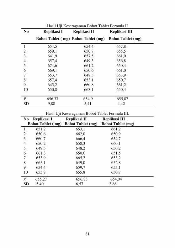
Hasil Uji Keseragaman Bobot Tablet Formula II
No Replikasi I Replikasi II Replikasi III
Bobot Tablet ( mg) Bobot Tablet (mg) Bobot Tablet (mg)
1 654,5 654,4 657,8 2 659,1 650,7 655,5 3 641,9 657,5 661,0 4 657,4 649,3 656,8 5 674,6 661,2 650,4 6 669,1 650,6 661,0 7 653,7 648,3 653,9 8 657,4 653,1 650,7 9 645,2 660,8 661,2 10 650,8 663,1 650,4
HI 656,37 654,9 655,87 SD 9,88 5,41 4,42
Hasil Uji Keseragaman Bobot Tablet Formula III.
No Replikasi I Replikasi II Replikasi III
Bobot Tablet ( mg) Bobot Tablet (mg) Bobot Tablet (mg)
1 651,2 653,1 661,2 2 650,6 662,0 650,9 3 660,7 666,4 654,7 4 650,2 658,3 660,1 5 649,5 648,2 650,2 6 661,3 650,6 651,5 7 653,9 665,2 653,2 8 665,1 649,0 652,8 9 654,4 659,7 655,1 10 655,8 655,8 650,7
HI 655,27 656,83 654,04 SD 5,40 6,57 3,86
82
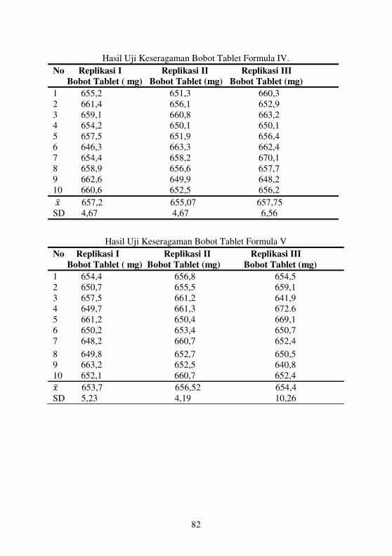
Hasil Uji Keseragaman Bobot Tablet Formula IV.
No Replikasi I Replikasi II Replikasi III
Bobot Tablet ( mg) Bobot Tablet (mg) Bobot Tablet (mg)
1 655,2 651,3 660,3 2 661,4 656,1 652,9 3 659,1 660,8 663,2 4 654,2 650,1 650,1 5 657,5 651,9 656,4 6 646,3 663,3 662,4 7 654,4 658,2 670,1 8 658,9 656,6 657,7 9 662,6 649,9 648,2 10 660,6 652,5 656,2
HI 657,2 655,07 657,75 SD 4,67 4,67 6,56
Hasil Uji Keseragaman Bobot Tablet Formula V
No Replikasi I Replikasi II Replikasi III
Bobot Tablet ( mg) Bobot Tablet (mg) Bobot Tablet (mg)
1 654,4 656,8 654,5 2 650,7 655,5 659,1 3 657,5 661,2 641,9 4 649,7 661,3 672.6 5 661,2 650,4 669,1 6 650,2 653,4 650,7 7 648,2 660,7 652,4
8 649,8 652,7 650,5 9 663,2 652,5 640,8 10 652,1 660,7 652,4
HI 653,7 656,52 654,4 SD 5,23 4,19 10,26
83
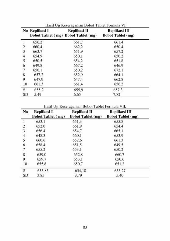
Hasil Uji Keseragaman Bobot Tablet Formula VI
No Replikasi I Replikasi II Replikasi III
Bobot Tablet ( mg) Bobot Tablet (mg) Bobot Tablet (mg)
1 656,2 661,7 661,4 2 660,4 662,2 650,4 3 663,7 651,9 657,2 4 654,9 650,1 650,2 5 650,5 654,2 651,8 6 649,8 667,2 646,9 7 650,1 650,2 672,1 8 657,2 652,9 664,1 9 647,9 647,4 662,8 10 661,3 661,4 656,2
HI 655,2 655,9 657,3 SD 5,49 6,65 7,82
Hasil Uji Keseragaman Bobot Tablet Formula VII.
No Replikasi I Replikasi II Replikasi III
Bobot Tablet ( mg) Bobot Tablet (mg) Bobot Tablet (mg)
1 653,1 651,3 655,8 2 652,0 661,9 654,4 3 656,4 654,7 665,1 4 648,3 660,1 653,9 5 660,6 652,6 661,3 6 658,4 651,5 649,5 7 655,2 653,1 650,2
8 659,0 652,8 660,7 9 659,7 653,1 650,6 10 655,8 650,7 651,2
HI 655,85 654,18 655,27 SD 3,85 3,79 5,40
84
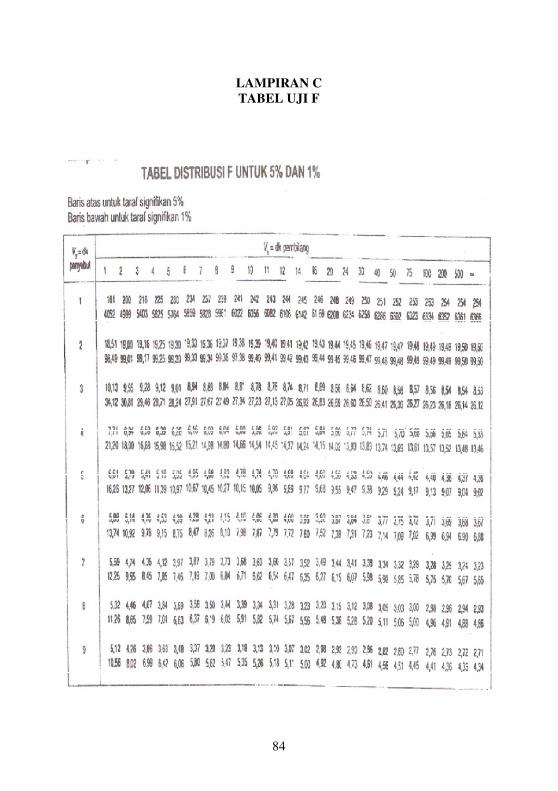
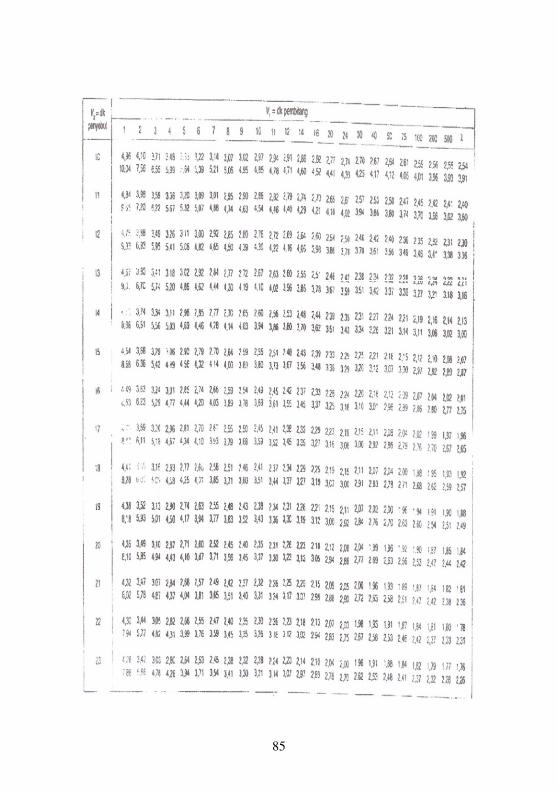
LAMPIRAN C
TABEL UJI F
85
86
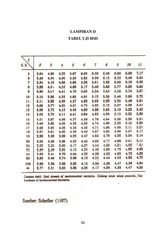
LAMPIRAN D
TABEL UJI HSD
87
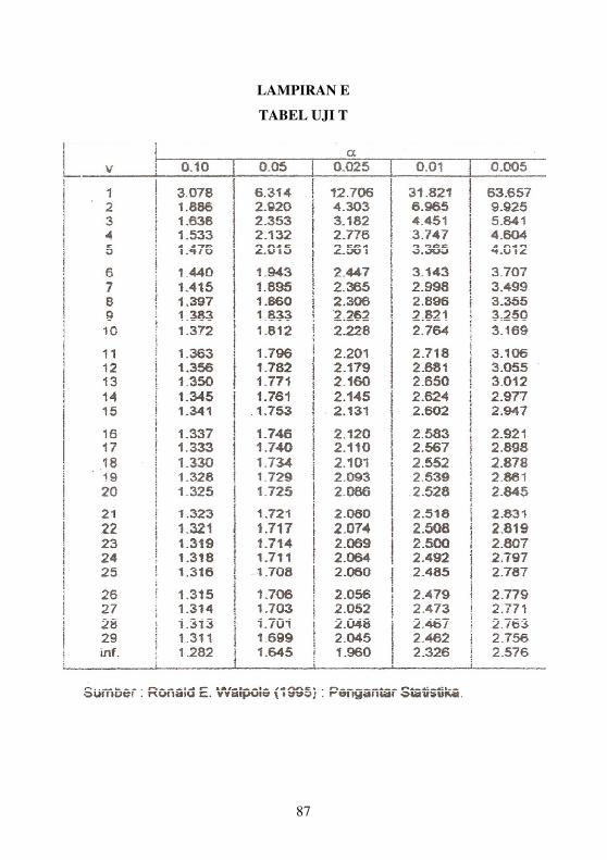
LAMPIRAN E
TABEL UJI T
88
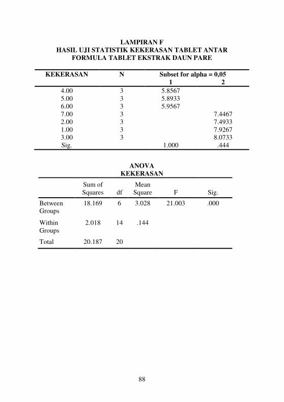
LAMPIRAN F
HASIL UJI STATISTIK KEKERASAN TABLET ANTAR
FORMULA TABLET EKSTRAK DAUN PARE
KEKERASAN N Subset for alpha = 0,05
1 2
4.00 3 5.8567 5.00 3 5.8933 6.00 3 5.9567 7.00 3 7.4467 2.00 3 7.4933 1.00 3 7.9267 3.00 3 8.0733 Sig. 1.000 .444
ANOVA
KEKERASAN
Sum of Squares df
Mean Square F Sig.
Between Groups
18.169 6 3.028 21.003 .000
Within Groups
2.018 14 .144
Total 20.187 20
89
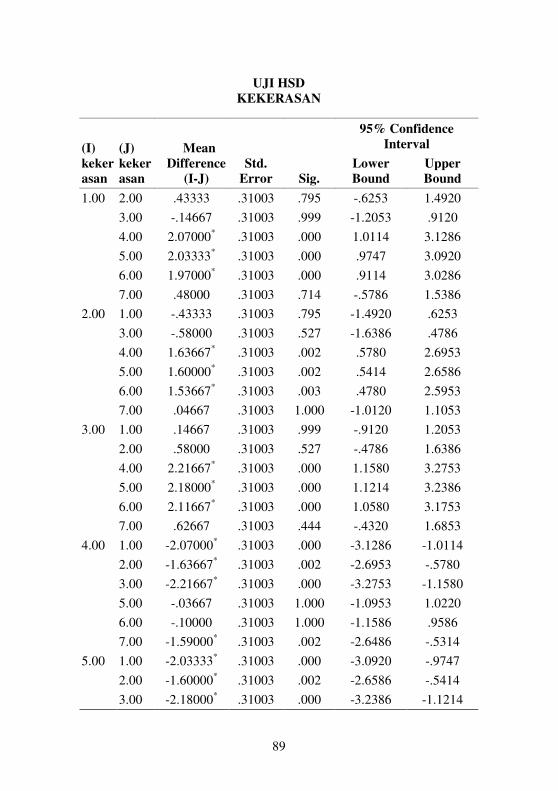
UJI HSD
KEKERASAN
(I)
keker
asan
(J)
keker
asan
Mean
Difference
(I-J)
Std.
Error Sig.
95% Confidence
Interval
Lower
Bound
Upper
Bound
1.00 2.00 .43333 .31003 .795 -.6253 1.4920
3.00 -.14667 .31003 .999 -1.2053 .9120
4.00 2.07000* .31003 .000 1.0114 3.1286
5.00 2.03333* .31003 .000 .9747 3.0920
6.00 1.97000* .31003 .000 .9114 3.0286
7.00 .48000 .31003 .714 -.5786 1.5386
2.00 1.00 -.43333 .31003 .795 -1.4920 .6253
3.00 -.58000 .31003 .527 -1.6386 .4786
4.00 1.63667* .31003 .002 .5780 2.6953
5.00 1.60000* .31003 .002 .5414 2.6586
6.00 1.53667* .31003 .003 .4780 2.5953
7.00 .04667 .31003 1.000 -1.0120 1.1053
3.00 1.00 .14667 .31003 .999 -.9120 1.2053
2.00 .58000 .31003 .527 -.4786 1.6386
4.00 2.21667* .31003 .000 1.1580 3.2753
5.00 2.18000* .31003 .000 1.1214 3.2386
6.00 2.11667* .31003 .000 1.0580 3.1753
7.00 .62667 .31003 .444 -.4320 1.6853
4.00 1.00 -2.07000* .31003 .000 -3.1286 -1.0114
2.00 -1.63667* .31003 .002 -2.6953 -.5780
3.00 -2.21667* .31003 .000 -3.2753 -1.1580
5.00 -.03667 .31003 1.000 -1.0953 1.0220
6.00 -.10000 .31003 1.000 -1.1586 .9586
7.00 -1.59000* .31003 .002 -2.6486 -.5314
5.00 1.00 -2.03333* .31003 .000 -3.0920 -.9747
2.00 -1.60000* .31003 .002 -2.6586 -.5414
3.00 -2.18000* .31003 .000 -3.2386 -1.1214
90
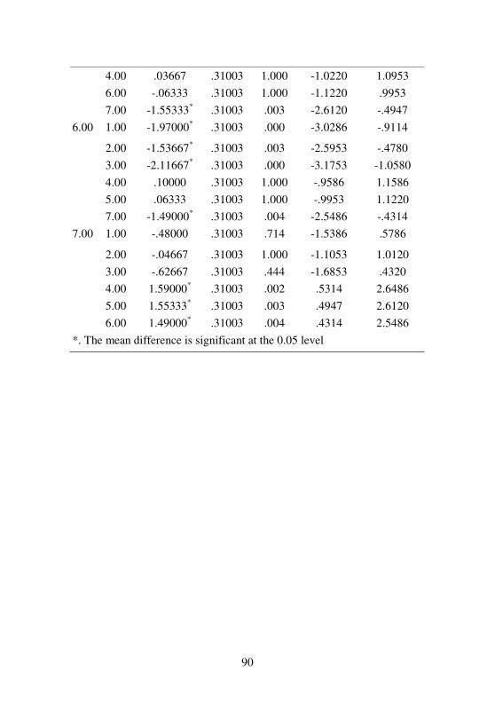
4.00 .03667 .31003 1.000 -1.0220 1.0953
6.00 -.06333 .31003 1.000 -1.1220 .9953
7.00 -1.55333* .31003 .003 -2.6120 -.4947
6.00 1.00 -1.97000* .31003 .000 -3.0286 -.9114
2.00 -1.53667* .31003 .003 -2.5953 -.4780
3.00 -2.11667* .31003 .000 -3.1753 -1.0580
4.00 .10000 .31003 1.000 -.9586 1.1586
5.00 .06333 .31003 1.000 -.9953 1.1220
7.00 -1.49000* .31003 .004 -2.5486 -.4314
7.00 1.00 -.48000 .31003 .714 -1.5386 .5786
2.00 -.04667 .31003 1.000 -1.1053 1.0120
3.00 -.62667 .31003 .444 -1.6853 .4320
4.00 1.59000* .31003 .002 .5314 2.6486
5.00 1.55333* .31003 .003 .4947 2.6120
6.00 1.49000* .31003 .004 .4314 2.5486
*. The mean difference is significant at the 0.05 level
91
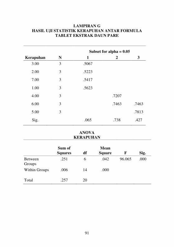
LAMPIRAN G
HASIL UJI STATISTIK KERAPUHAN ANTAR FORMULA
TABLET EKSTRAK DAUN PARE
Kerapuhan N
Subset for alpha = 0.05
1 2 3
3.00 3 .5067
2.00 3 .5223
7.00 3 .5417
1.00 3 .5623
4.00 3 .7207
6.00 3 .7463 .7463
5.00 3 .7813
Sig. .065 .738 .427
ANOVA
KERAPUHAN
Sum of
Squares df
Mean
Square F Sig.
Between Groups
.251 6 .042 96.065 .000
Within Groups .006 14 .000
Total .257 20
92
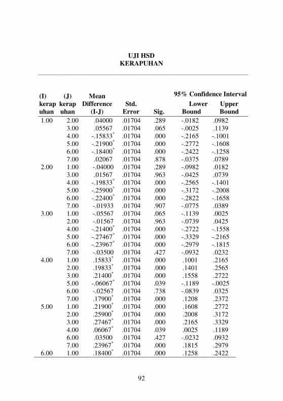
UJI HSD
KERAPUHAN
(I)
kerap
uhan
(J)
kerap
uhan
Mean
Difference
(I-J)
Std.
Error
Sig.
95% Confidence Interval
Lower
Bound
Upper
Bound
1.00 2.00 .04000 .01704 .289 -.0182 .0982 3.00 .05567 .01704 .065 -.0025 .1139 4.00 -.15833* .01704 .000 -.2165 -.1001 5.00 -.21900* .01704 .000 -.2772 -.1608 6.00 -.18400* .01704 .000 -.2422 -.1258 7.00 .02067 .01704 .878 -.0375 .0789
2.00 1.00 -.04000 .01704 .289 -.0982 .0182 3.00 .01567 .01704 .963 -.0425 .0739 4.00 -.19833* .01704 .000 -.2565 -.1401 5.00 -.25900* .01704 .000 -.3172 -.2008 6.00 -.22400* .01704 .000 -.2822 -.1658 7.00 -.01933 .01704 .907 -.0775 .0389
3.00 1.00 -.05567 .01704 .065 -.1139 .0025 2.00 -.01567 .01704 .963 -.0739 .0425 4.00 -.21400* .01704 .000 -.2722 -.1558 5.00 -.27467* .01704 .000 -.3329 -.2165 6.00 -.23967* .01704 .000 -.2979 -.1815 7.00 -.03500 .01704 .427 -.0932 .0232
4.00 1.00 .15833* .01704 .000 .1001 .2165 2.00 .19833* .01704 .000 .1401 .2565 3.00 .21400* .01704 .000 .1558 .2722 5.00 -.06067* .01704 .039 -.1189 -.0025 6.00 -.02567 .01704 .738 -.0839 .0325 7.00 .17900* .01704 .000 .1208 .2372
5.00 1.00 .21900* .01704 .000 .1608 .2772 2.00 .25900* .01704 .000 .2008 .3172 3.00 .27467* .01704 .000 .2165 .3329 4.00 .06067* .01704 .039 .0025 .1189 6.00 .03500 .01704 .427 -.0232 .0932 7.00 .23967* .01704 .000 .1815 .2979
6.00 1.00 .18400* .01704 .000 .1258 .2422
93
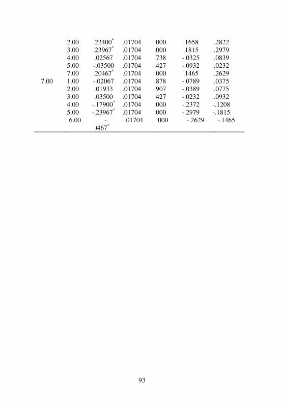
2.00 .22400* .01704 .000 .1658 .2822 3.00 .23967* .01704 .000 .1815 .2979 4.00 .02567 .01704 .738 -.0325 .0839 5.00 -.03500 .01704 .427 -.0932 .0232 7.00 .20467* .01704 .000 .1465 .2629
7.00 1.00 -.02067 .01704 .878 -.0789 .0375 2.00 .01933 .01704 .907 -.0389 .0775 3.00 .03500 .01704 .427 -.0232 .0932 4.00 -.17900* .01704 .000 -.2372 -.1208 5.00 -.23967* .01704 .000 -.2979 -.1815 6.00 -
.20467* .01704 .000 -.2629 -.1465
94
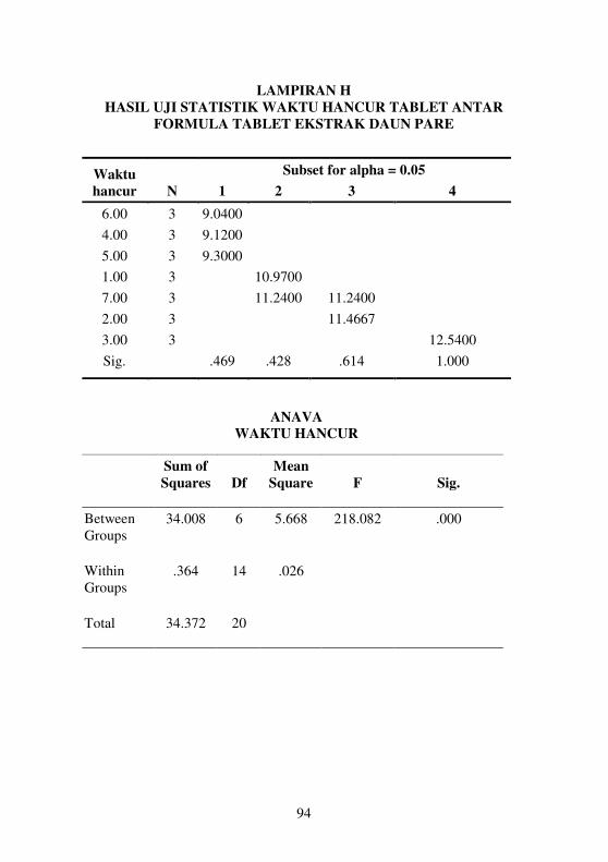
LAMPIRAN H
HASIL UJI STATISTIK WAKTU HANCUR TABLET ANTAR
FORMULA TABLET EKSTRAK DAUN PARE
Waktu
hancur N
Subset for alpha = 0.05
1 2 3 4
6.00 3 9.0400
4.00 3 9.1200
5.00 3 9.3000
1.00 3 10.9700
7.00 3 11.2400 11.2400
2.00 3 11.4667
3.00 3 12.5400
Sig. .469 .428 .614 1.000
ANAVA
WAKTU HANCUR
Sum of
Squares Df
Mean
Square F Sig.
Between
Groups 34.008 6 5.668 218.082 .000
Within
Groups .364 14 .026
Total 34.372 20
95
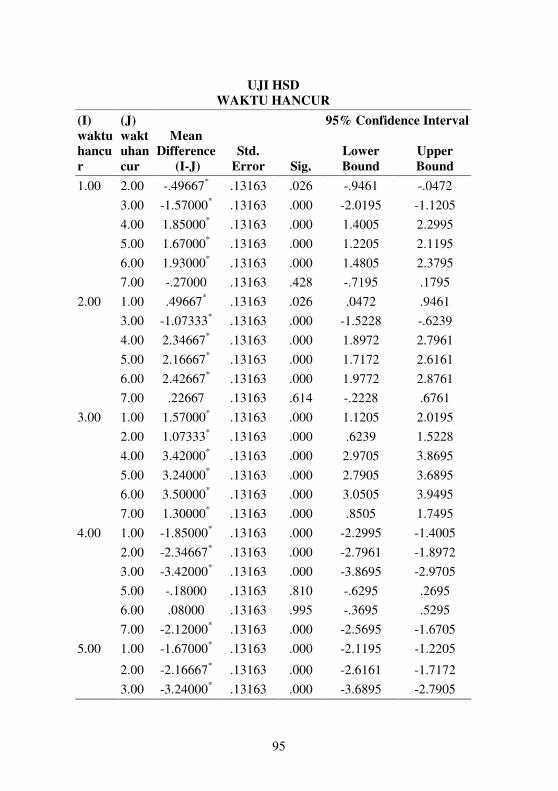
UJI HSD
WAKTU HANCUR
(I)
waktu
hancu
r
(J)
wakt
uhan
cur
Mean
Difference
(I-J)
Std.
Error Sig.
95% Confidence Interval
Lower
Bound
Upper
Bound
1.00 2.00 -.49667* .13163 .026 -.9461 -.0472
3.00 -1.57000* .13163 .000 -2.0195 -1.1205
4.00 1.85000* .13163 .000 1.4005 2.2995
5.00 1.67000* .13163 .000 1.2205 2.1195
6.00 1.93000* .13163 .000 1.4805 2.3795
7.00 -.27000 .13163 .428 -.7195 .1795
2.00 1.00 .49667* .13163 .026 .0472 .9461
3.00 -1.07333* .13163 .000 -1.5228 -.6239
4.00 2.34667* .13163 .000 1.8972 2.7961
5.00 2.16667* .13163 .000 1.7172 2.6161
6.00 2.42667* .13163 .000 1.9772 2.8761
7.00 .22667 .13163 .614 -.2228 .6761
3.00 1.00 1.57000* .13163 .000 1.1205 2.0195
2.00 1.07333* .13163 .000 .6239 1.5228
4.00 3.42000* .13163 .000 2.9705 3.8695
5.00 3.24000* .13163 .000 2.7905 3.6895
6.00 3.50000* .13163 .000 3.0505 3.9495
7.00 1.30000* .13163 .000 .8505 1.7495
4.00 1.00 -1.85000* .13163 .000 -2.2995 -1.4005
2.00 -2.34667* .13163 .000 -2.7961 -1.8972
3.00 -3.42000* .13163 .000 -3.8695 -2.9705
5.00 -.18000 .13163 .810 -.6295 .2695
6.00 .08000 .13163 .995 -.3695 .5295
7.00 -2.12000* .13163 .000 -2.5695 -1.6705
5.00 1.00 -1.67000* .13163 .000 -2.1195 -1.2205
2.00 -2.16667* .13163 .000 -2.6161 -1.7172
3.00 -3.24000* .13163 .000 -3.6895 -2.7905
96
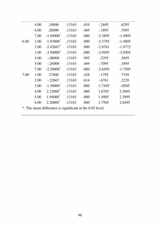
4.00 .18000 .13163 .810 -.2695 .6295
6.00 .26000 .13163 .469 -.1895 .7095
7.00 -1.94000* .13163 .000 -2.3895 -1.4905
6.00 1.00 -1.93000* .13163 .000 -2.3795 -1.4805
2.00 -2.42667* .13163 .000 -2.8761 -1.9772
3.00 -3.50000* .13163 .000 -3.9495 -3.0505
4.00 -.08000 .13163 .995 -.5295 .3695
5.00 -.26000 .13163 .469 -.7095 .1895
7.00 -2.20000* .13163 .000 -2.6495 -1.7505
7.00 1.00 .27000 .13163 .428 -.1795 .7195
2.00 -.22667 .13163 .614 -.6761 .2228
3.00 -1.30000* .13163 .000 -1.7495 -.8505
4.00 2.12000* .13163 .000 1.6705 2.5695
5.00 1.94000* .13163 .000 1.4905 2.3895
6.00 2.20000* .13163 .000 1.7505 2.6495
*. The mean difference is significant at the 0.05 level.
97
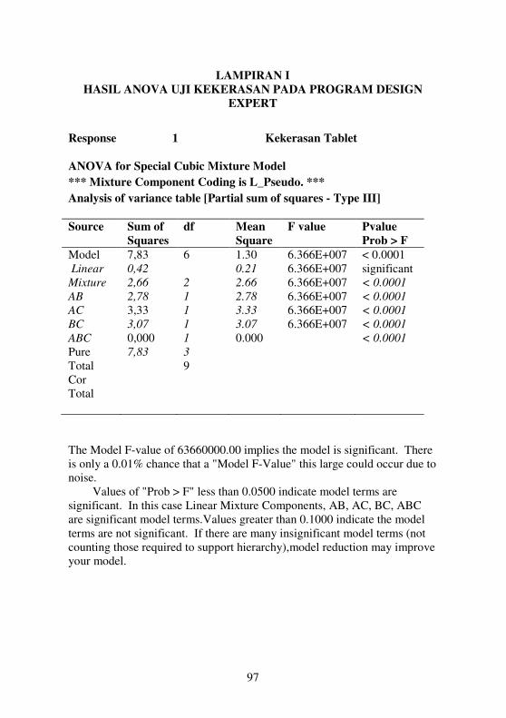
LAMPIRAN I
HASIL ANOVA UJI KEKERASAN PADA PROGRAM DESIGN
EXPERT
Response 1 Kekerasan Tablet
ANOVA for Special Cubic Mixture Model
*** Mixture Component Coding is L_Pseudo. ***
Analysis of variance table [Partial sum of squares - Type III]
Source
Sum of
Squares
df Mean
Square
F value Pvalue
Prob > F
Model Linear
Mixture AB AC
BC ABC
Pure Total Cor Total
7,83 0,42 2,66 2,78 3,33 3,07 0,000 7,83
6 2 1 1 1 1
3 9
1.30 0.21 2.66 2.78 3.33 3.07 0.000
6.366E+007 6.366E+007 6.366E+007 6.366E+007 6.366E+007 6.366E+007
< 0.0001 significant < 0.0001 < 0.0001 < 0.0001 < 0.0001 < 0.0001
The Model F-value of 63660000.00 implies the model is significant. There is only a 0.01% chance that a "Model F-Value" this large could occur due to noise. Values of "Prob > F" less than 0.0500 indicate model terms are significant. In this case Linear Mixture Components, AB, AC, BC, ABC are significant model terms.Values greater than 0.1000 indicate the model terms are not significant. If there are many insignificant model terms (not counting those required to support hierarchy),model reduction may improve your model.
98
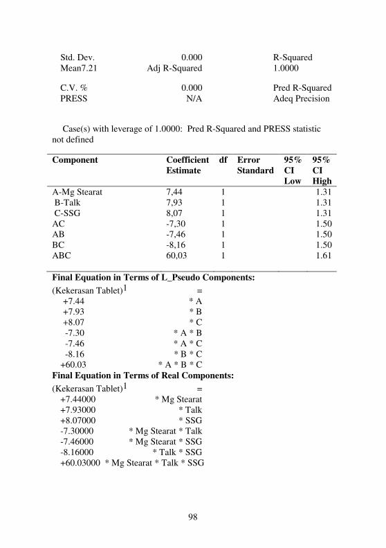
Std. Dev. 0.000 R-Squared
Mean7.21 Adj R-Squared 1.0000
C.V. % 0.000 Pred R-Squared
PRESS N/A Adeq Precision
Case(s) with leverage of 1.0000: Pred R-Squared and PRESS statistic
not defined
Component Coefficient Estimate
df Error Standard
95%
CI
Low
95%
CI
High
A-Mg Stearat B-Talk C-SSG AC AB BC ABC
7,44 7,93 8,07 -7,30 -7,46 -8,16 60,03
1 1 1 1 1 1 1
1.31 1.31 1.31 1.50 1.50 1.50 1.61
Final Equation in Terms of L_Pseudo Components:
(Kekerasan Tablet)1 = +7.44 * A +7.93 * B +8.07 * C -7.30 * A * B -7.46 * A * C -8.16 * B * C +60.03 * A * B * C
Final Equation in Terms of Real Components:
(Kekerasan Tablet)1 = +7.44000 * Mg Stearat +7.93000 * Talk +8.07000 * SSG -7.30000 * Mg Stearat * Talk -7.46000 * Mg Stearat * SSG -8.16000 * Talk * SSG +60.03000 * Mg Stearat * Talk * SSG
99
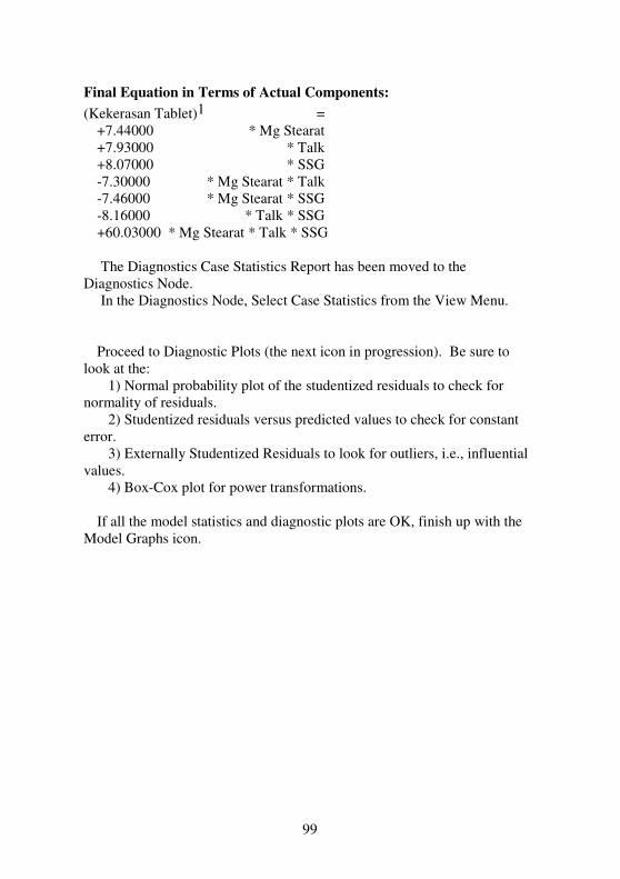
Final Equation in Terms of Actual Components:
(Kekerasan Tablet)1 = +7.44000 * Mg Stearat +7.93000 * Talk +8.07000 * SSG -7.30000 * Mg Stearat * Talk -7.46000 * Mg Stearat * SSG -8.16000 * Talk * SSG +60.03000 * Mg Stearat * Talk * SSG The Diagnostics Case Statistics Report has been moved to the Diagnostics Node. In the Diagnostics Node, Select Case Statistics from the View Menu. Proceed to Diagnostic Plots (the next icon in progression). Be sure to look at the: 1) Normal probability plot of the studentized residuals to check for normality of residuals. 2) Studentized residuals versus predicted values to check for constant error. 3) Externally Studentized Residuals to look for outliers, i.e., influential values. 4) Box-Cox plot for power transformations. If all the model statistics and diagnostic plots are OK, finish up with the Model Graphs icon.
100
LAMPIRAN J
HASIL ANOVA UJI KERAPUHAN PADA PROGRAM DESIGN
EXPERT
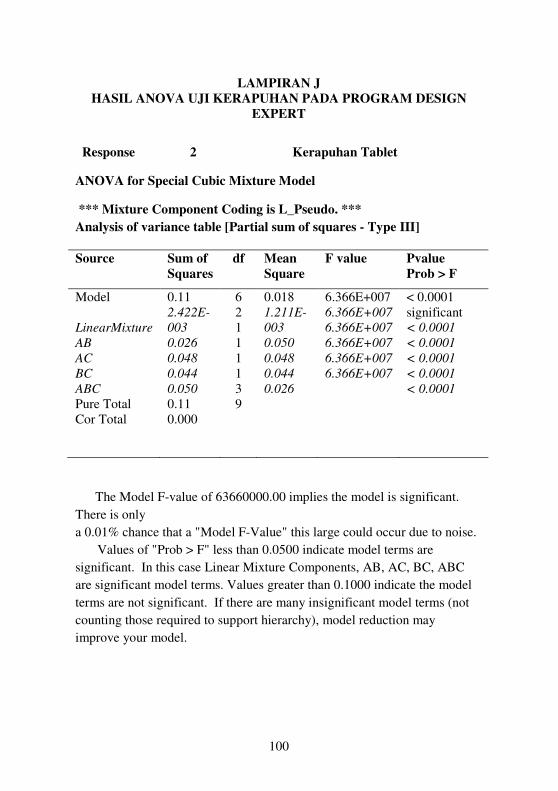
Response 2 Kerapuhan Tablet
ANOVA for Special Cubic Mixture Model
*** Mixture Component Coding is L_Pseudo. ***
Analysis of variance table [Partial sum of squares - Type III]
Source
Sum of
Squares
df Mean
Square
F value Pvalue
Prob > F
Model
LinearMixture AB AC
BC ABC
Pure Total Cor Total
0.11 2.422E-
003 0.026 0.048 0.044 0.050 0.11 0.000
6 2 1 1 1 1 3 9
0.018 1.211E-
003 0.050 0.048 0.044 0.026
6.366E+007 6.366E+007 6.366E+007 6.366E+007 6.366E+007 6.366E+007
< 0.0001 significant < 0.0001 < 0.0001 < 0.0001 < 0.0001 < 0.0001
The Model F-value of 63660000.00 implies the model is significant.
There is only
a 0.01% chance that a "Model F-Value" this large could occur due to noise.
Values of "Prob > F" less than 0.0500 indicate model terms are
significant. In this case Linear Mixture Components, AB, AC, BC, ABC
are significant model terms. Values greater than 0.1000 indicate the model
terms are not significant. If there are many insignificant model terms (not
counting those required to support hierarchy), model reduction may
improve your model.
101
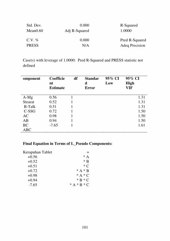
Std. Dev. 0.000 R-Squared
Mean0.60 Adj R-Squared 1.0000
C.V. % 0.000 Pred R-Squared
PRESS N/A Adeq Precision
Case(s) with leverage of 1.0000: Pred R-Squared and PRESS statistic not
defined
Final Equation in Terms of L_Pseudo Components:
Kerapuhan Tablet = +0.56 * A +0.52 * B +0.51 * C +0.72 * A * B +0.98 * A * C +0.94 * B * C
-7.65 * A * B * C
omponent Coefficie
nt Estimate
df Standar
d Error
95% CI
Low 95% CI
High VIF
A-Mg Stearat B-Talk C-SSG AC AB BC ABC
0.56 0.52 0.51 0.72 0.98 0.94 -7.65
1 1 1 1 1 1 1
1.31 1.31 1.31 1.50 1.50 1.50 1.61
102
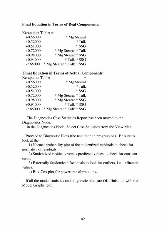
Final Equation in Terms of Real Components:
Kerapuhan Tablet = +0.56000 * Mg Stearat +0.52000 * Talk +0.51000 * SSG +0.72000 * Mg Stearat * Talk +0.98000 * Mg Stearat * SSG +0.94000 * Talk * SSG -7.65000 * Mg Stearat * Talk * SSG
Final Equation in Terms of Actual Components: Kerapuhan Tablet = +0.56000 * Mg Stearat +0.52000 * Talk +0.51000 * SSG +0.72000 * Mg Stearat * Talk +0.98000 * Mg Stearat * SSG +0.94000 * Talk * SSG -7.65000 * Mg Stearat * Talk * SSG The Diagnostics Case Statistics Report has been moved to the Diagnostics Node. In the Diagnostics Node, Select Case Statistics from the View Menu. Proceed to Diagnostic Plots (the next icon in progression). Be sure to look at the: 1) Normal probability plot of the studentized residuals to check for normality of residuals. 2) Studentized residuals versus predicted values to check for constant error. 3) Externally Studentized Residuals to look for outliers, i.e., influential values. 4) Box-Cox plot for power transformations. If all the model statistics and diagnostic plots are OK, finish up with the Model Graphs icon.
103
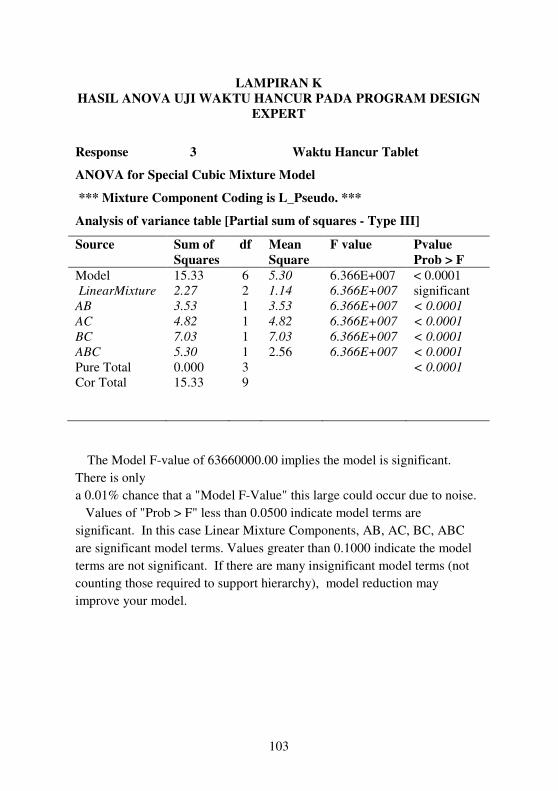
LAMPIRAN K
HASIL ANOVA UJI WAKTU HANCUR PADA PROGRAM DESIGN
EXPERT
Response 3 Waktu Hancur Tablet
ANOVA for Special Cubic Mixture Model
*** Mixture Component Coding is L_Pseudo. ***
Analysis of variance table [Partial sum of squares - Type III]
Source
Sum of
Squares
df Mean
Square
F value Pvalue
Prob > F
Model LinearMixture AB AC
BC ABC
Pure Total Cor Total
15.33 2.27 3.53 4.82 7.03 5.30 0.000 15.33
6 2 1 1 1 1 3 9
5.30 1.14 3.53 4.82 7.03 2.56
6.366E+007 6.366E+007 6.366E+007 6.366E+007 6.366E+007 6.366E+007
< 0.0001 significant < 0.0001 < 0.0001 < 0.0001 < 0.0001 < 0.0001
The Model F-value of 63660000.00 implies the model is significant.
There is only
a 0.01% chance that a "Model F-Value" this large could occur due to noise.
Values of "Prob > F" less than 0.0500 indicate model terms are
significant. In this case Linear Mixture Components, AB, AC, BC, ABC
are significant model terms. Values greater than 0.1000 indicate the model
terms are not significant. If there are many insignificant model terms (not
counting those required to support hierarchy), model reduction may
improve your model.
104
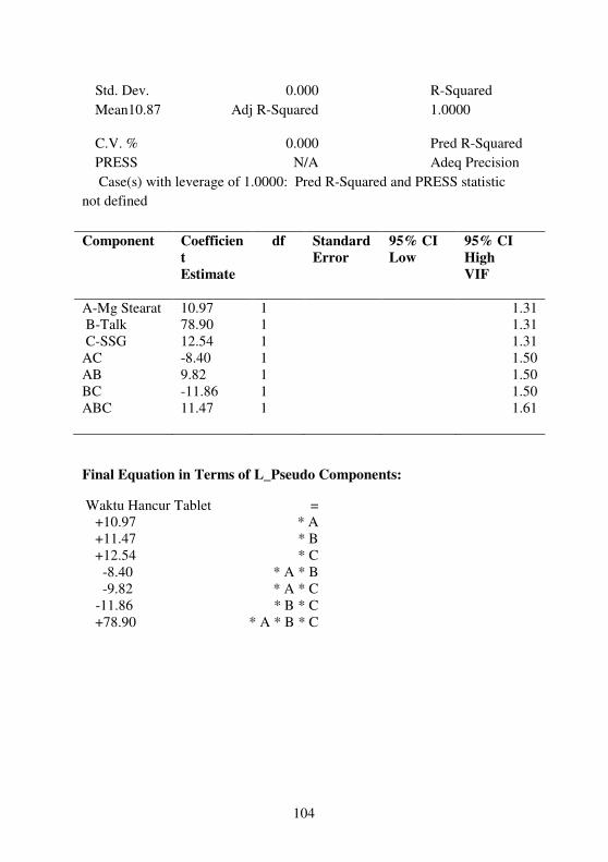
Std. Dev. 0.000 R-Squared
Mean10.87 Adj R-Squared 1.0000
C.V. % 0.000 Pred R-Squared
PRESS N/A Adeq Precision
Case(s) with leverage of 1.0000: Pred R-Squared and PRESS statistic
not defined
Final Equation in Terms of L_Pseudo Components:
Waktu Hancur Tablet = +10.97 * A +11.47 * B +12.54 * C -8.40 * A * B -9.82 * A * C -11.86 * B * C +78.90 * A * B * C
Component Coefficien
t Estimate
df Standard Error
95% CI
Low 95% CI
High VIF
A-Mg Stearat B-Talk C-SSG AC AB BC ABC
10.97 78.90 12.54 -8.40 9.82 -11.86 11.47
1 1 1 1 1 1 1
1.31 1.31 1.31 1.50 1.50 1.50 1.61
105
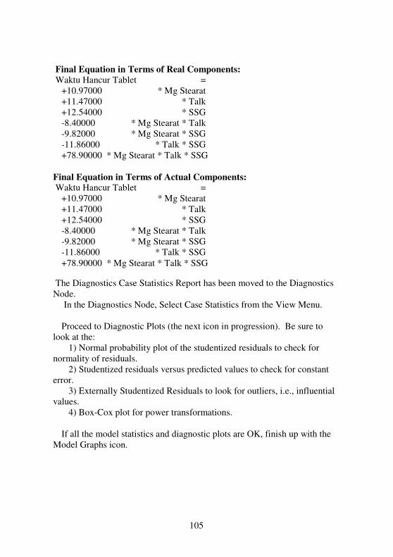
Final Equation in Terms of Real Components: Waktu Hancur Tablet = +10.97000 * Mg Stearat +11.47000 * Talk +12.54000 * SSG -8.40000 * Mg Stearat * Talk -9.82000 * Mg Stearat * SSG -11.86000 * Talk * SSG +78.90000 * Mg Stearat * Talk * SSG
Final Equation in Terms of Actual Components: Waktu Hancur Tablet = +10.97000 * Mg Stearat +11.47000 * Talk +12.54000 * SSG -8.40000 * Mg Stearat * Talk -9.82000 * Mg Stearat * SSG -11.86000 * Talk * SSG
+78.90000 * Mg Stearat * Talk * SSG
The Diagnostics Case Statistics Report has been moved to the Diagnostics Node. In the Diagnostics Node, Select Case Statistics from the View Menu. Proceed to Diagnostic Plots (the next icon in progression). Be sure to look at the: 1) Normal probability plot of the studentized residuals to check for normality of residuals. 2) Studentized residuals versus predicted values to check for constant error. 3) Externally Studentized Residuals to look for outliers, i.e., influential values. 4) Box-Cox plot for power transformations. If all the model statistics and diagnostic plots are OK, finish up with the Model Graphs icon.
106
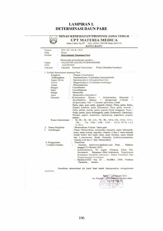
LAMPIRAN L
DETERMINASI DAUN PARE
107
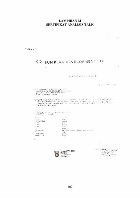
LAMPIRAN M
SERTIFIKAT ANALISIS TALK

108
LAMPIRAN N
SERTIFIKAT ANALISIS MAGNESIUM STEARAT
109
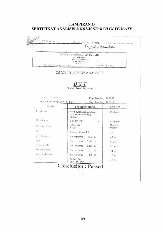
LAMPIRAN O
SERTIFIKAT ANALISIS SODIUM STARCH GLYCOLATE