UNIVERSITI SAINS MALAYSIA

Laporan Akhir Projek PenyelidikanJangka Pendek

Tool Wear Measurement Using MachineVision

byAssoc. Prof. Dr. Mani Maran all Ratnam

.,.

2008

Project title:

Project leader:

USM SHORT TERM GRANT

COMPREHENSIVE REPORT

Tool wear measurement using machine vision

Dr. Mani Maran a/I RatnamSchool of Mechanical EngineeringUniversiti Sains Malaysia,Engineering Campus,14300 Nibong Tebal,Penang.

Duration of project: 15 Mei 2006 -14 Mei 2008

Contents:

1. Introduction

1.1 Project Description

1.2 Project Activities

1.3 Project Benefits

1.4 Project Duration

1.5 Approved Grant Amount

1.6 Project Cost

2. Project Contribution/Achievement

2.1 Thesis and publications

2.2 Award

3. Conclusion

4. Acknowledgement

2

1. Introduction

1.1 Project Description

In any machining operation, tool wear changes the geometry of cutting

tools and decreases the dimensional accuracy and surface finish of the product.

Monitoring of tool wear is an important for enhancing productivity in machining

operations. Many investigators worldwide have studied tool wear as a significant

area of research.

There are two main methods of estimating tool wear: (i) Indirect method

and (ii) direct method. Examples of indirect methods are acoustic emission, tool tip

temperature monitoring, vibration signatures and cutting force monitoring. Such

methods require sophisticated and expensive devices and instrument and are,

therefore, difficult to use in the workshop environment. Direct methods include use

of toolmaker's microscope and profile projector to directly measure tool wear.

Recently, vision systems are being exploited for such application mainly

due to their high resolution, reliability and ease of automatic processing of data.

Such systems are also being used with special lighting techniques to measure tool

wear in 3-D. In spite of the large amount of work worldwide on the application of

machine vision for tool wear monitoring, such system have been mostly

implemented on computer-numerical-control (CNC) lathe and milling machines.

This is because of the need to park and align the cutting tool precisely under the

field of view of the camera for accurate wear measurement. Such requirement

limits the application of such techniques only to CNC machines.

This objective of this project is to develop a tool wear measurement system.,.

using machine vision that can measure tool nose wear by automatically performing

software correction of misalignment of the tool insert. The system developed was

intended to 'be used in machine tool workshops to monitor tool wear and change

the cutting tool at an optimum time, thus reducing damage to work piece.

The technique developed is able to remove the constraints of other vision

based techniques developed worldwide to measure tool wear in which the systems

are limited for use on CNC machines. The software correction of misalignment

3

proposed in this research is able to remove the constraint and permit application to

conventional lathe machines.

1.2 Project Activities

The methodology in the research involves the various stages of work described

below:

Stage 1: Literature study

This part of the work involves a literature study on the state-of-the art research

worldwide on the application of machine vision in tool wear measurement in lathe

machining operations.

Stage 2: Setup of machine vision system and calibration

In this stage of the work, machine vision system, comprising a CCD camera, frame

grabber and personal computer will be set up using existing hardware (purchased

in a previous IRPA funded project). Suitable tool fixtures will be developed to

position the tool under the camera and introduce rotational and translational

misalignment. A study will be carried out to determine the maximum resolution that

can be obtained using various lenses and extension tubes.

Stage 3: Machining operations using conventional lathe

In this stage of the work, several machining operations will be carried out using

different feed rates and spindle speeds. The objective of this work is to prepare the

specimens for subsequent experiments.

Stage 4: Development of algorithms to measure tool wear in the presence of

m'isalignment

This part of the work focuses on the development of algorithms (in Matlab) to

measure tool wear in the presence of rotational and translational misalignment. A

study will be carried out to identify suitable pre-processing stages necessary to

improve accuracy of the tool wear measurement. The measurement results will be

4

compared with other techniques, such as toolmaker's microscope and profile

projector.

Stage 5: Development of fixture to mount camera and lighting system of lathe

machine

In this part of the work, suitable fixtures will be design and developed to mount the

camera and lighting system onto the lathe machine for real-time measurement.

Stage 6: Real-time tool wear measurement

Real-time tool wear measurement will be attempted using the hardware and

algorithms developed in this research in this stage of the work.

Stage 7: Study on effect of machining parameters on tool wear

In this final stage of work, a study will be carried out on the effect of machining

parameters on tool wear. The possibility of measuring tool wear in the presence of

misalignment will be demonstrated.

The various stages of the work are reported in the papers published and

the theses produced from this research (in preparation). Detailed reports on these

are available in the Appendix.

1.3 Project Benefits

The project benefits are as follows:

1. A new method of monitoring and measuring tool nose wear have been

developed. This method can be used by tool manufacturers to assess

the wear resistance of cutting tools under different machining

conditions.

2. A non-contact method of measuring the roughness of the finished

product!has also been developed as part of the research. This method

5

allows operators to quickly assess the roughness of workpiece without

removing it from the machine.

3. A method of assessing flank wear from the nose wear area has also

been proposed. This method can be used to assess flank wear without

removing the tool from the machine.

1.4 Project Duration

This project started in May 2006 and was completed in May 2006, that is,

for duration of two years.

1.5 Approved Grant Amount

The total amount approved under the short-term grant for this project is

RM14,034.00, which was disbursed in two installments.

1.6 Project Cost

The total amount spent for this project was RM13,469.76 with a balance of

RM564.24.

2. Project Contribution/Achievement

2.1 Theses and publications

The contribution of this research in terms of theses and publications are as follows:

PhD thesis:

1) Thesis titled: Study on the effect of tool nose wear on the surface roughness

and dimensional deviation of workpiece in finish turning using machine vision

- Hamidreza H Shahabi (to be submitted in August 2008).

6

Journal papers:

Papers published:

1. H.H.Shahabi, M.M.Ratnam, 'On-line monitoring of tool wear in turningoperation in the presence of tool misalignment', Int J of Adv Manf Tech, 00110.1 007/s00170-007-1119-4, (2007).

2. H. H. Shahabi, M. M. Ratnam, 'In-cycle monitoring of tool nose wear andsurface roughness of turned parts using machine vision', Int J of Adv ManfTech, 00110.1007/s00170-008-1430-8 (2008).

3. H.H. Shahabi, T.H. Low, M.M. Ratnam, 'Notch wear detection in cutting toolsusing gradient approach and polynomial fitting, Int J of Adv Manf Tech, 00110.1007/s00170-008-1437-1 (2008).

Papers under review:

1. H.H. Shahabi, M.M Ratnam, 'Assessment of flank wear and nose radius wearfrom workpiece roughness profile in turning operation using machine vision',submitted to fnt J ofAdv Manf Tech.

2. W.K. Mook, H.H. Shahabi, M.M Ratnam, 'Measurement of nose radius wear inturning tools from a single 2-D image using machine vision', submitted to Int Jof Adv Manf Tech.

Copies of the full papers are available in the Appendix attached to this report.

2.2 Award

A bronze medal was won for the product titled 'TooIMon: Tool wear

monitoring and measurement system for lathe machine' in ITEX2007 held from 18­

20 May 2007 in Kuala Lumpur. (Copy of certificate included in the Appendix).

3. Conclusion

A tool wear measurement system using machine vision has been

successfully developed in this research. Automatic software correction of tool

misalignment allows the system to be used in-cycle in the workshop environment.

Measurement can be carried out without removal of the cutting tool from the

machine. The system can also be used to measure workpiece roughness without

contact with the workpiece.

7

4. Acknowledgement

I would like to convey my sincere thanks to Universiti Sains Malaysia for the offer

of the short-term grant that has enabled this research to be carried out and completed

successfully.

Report prepared by:

Dr. Mani Maran a/I Ratnam (Project leader)Associate Professor,School of Mechanical Engineering,Engineering Campus,Universiti Sains Malaysia,14300 Nibong Tebal,Penang.

8

Appendix

9

lot J Adv Manuf TechnolDOII0.I007/s00170-008-1430-8

In-cycle monitoring of tool nose wear and surface roughnessof turned parts using machine vision

H. H. Shahabi • M. M. Ratnam

Received: 14 June 2007/ Accepted: 4 February 2008(!;;) Springer-Verlag London Limited 2008

Abstract Tool wear has been extensively studied in the pastdue to its effect on the surface quality of the finished product.Vision-based systems using a CCD camera are increasinglybeing used for measurement oftool wear due to their numerousadvantages compared to indirect methods. Most research intotool wear monitoring using vision systems focusses on off-linemeasurement ofwear. The effect ofwear on surface roughnessof the workpiece is also studied by measuring the roughnessoff-line using mechanical stylus methods. In this work, a visionsystem using a CCD camera and backlight was developed tomeasure the surface roughness of the turned part withoutremoving it from the machine in-between cutting processes,i.e. in-cycle. An algorithm developed in previous work wasused to automatically correct tool misalignment using theimages and measure the nose wear area. The surface roughnessof turned parts measured using the machine vision system wasverified using the mechanical stylus method. The nose wearwas measured for different feed rates and its effect on thesmface roughness of the turned part was studied. The resultsshowed that surface roughness initially decreased as themachining time of the tool increased due to increasing nosewear and then increased when notch wear occun·ed.

Keywords Machine vision· Tool wear· Surface roughness

1 Introduction

Tool wear and tool failure are among the limitations tounattended machining in modem manufacturing. In fact,

H. H. Shahabi . M. M. Ratnam ((g)School of Mechanical Engineering, Engineering Campus,Universiti Sains Malaysia,14300 Nibong Tcbal, Penang, Malaysiae-mail: mmaran@eng.usm.my

20% of the downtime of machine tools is reported to be dueto tool failure [1]. Thus, in order to save machining coststhe manufacturer has to replace worn out cutting tools 'just­in-time'. In-process (or on-line) monitoring of tool wear istherefore important in determining the best time to changethe cutting tool.

Several methods of monitoring and measuring tool wearhave been developed in the past. These can be broadlydivided into two groups: indirect methods and directmethods. Examples of indirect methods include acousticemission monitoring, tool-tip temperature monitoring,vibration signature analysis (acceleration signals), monitor­ing of motor current, and cutting force monitoring [2].These methods normally require expensive instrumentationand are difficult to implement in a typical workshopenvironment. Direct methods, such as machine visionsystems 'using a charged-couple-device (CCD) camera oroptical microscope, are able to measure tool wear directly.They are simpler and require less costly equipmentcompared to the indirect methods. Therefore, the applica­tion of machine vision to measurement of tool wear hasbeen of great interest in the research community in recentyears [1, 3-14].

The effect of tool wear on the surface quality ofmachined parts is well known [13-14]. The ease ofc~pturing and analyzing images of machined surfaces hasencouraged researchers in the past to use roughnessparameters for tool wear monitoring. Analysis of surfacetexture is one method of distinguishing a sharp tool fi'om aworn out tool [12]. The surface roughness can also bemeasured directly using mechanical stylus methods. Al­though the stylus method is accurate it has severaldisadvantages. For example, the stylus and its transducerare delicate and thus the instruments must be used in afairly vibration-free environment, and the method is slow

©Springer

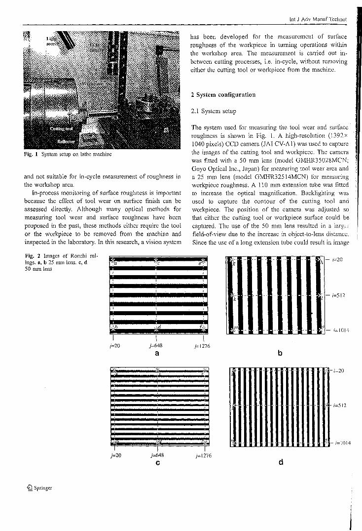
Fig. 1 System setup on lathe machine

and not suitable for in-cycle measurement of roughness inthe workshop area.

In-process monitoring of surface roughness is impoltantbecause the effect of tool wear on surface finish can beassessed directly. Although many optical methods formeasUling tool wear and surface roughness have beenproposed in the past, these methods either require the toolor the workpiece to be removed from the machine andinspected in the laboratory. In this research, a vision system

tnt J Adv Manuf Technol

has been developed for the measurement of surfaceroughness of the workpiece in turning operations withinthe workshop area. The measurement is carried out in­between cutting processes, i.e. in-cycle, without removingeither the cutting tool or workpiece from the machine.

2 System configuration

2.1 System setup

The system used for measuring the tool wear and surfaceroughness is shown in Fig. 1. A high-resolution (1392 x

1040 pixels) CCD camera (JAI CV-A1) was used to capturethe images of the cutting tool and workpiece. The camerawas fitted with a 50 mm lens (model GMHR35028MCN;Goyo Optical Inc., Japan) for measuring tool wear area anda 25 mm lens (model GMHR32514MCN) for measuringworkpiece roughness. A 110 mm extension tube was fittedto increase the optical magnification. Backlighting wasused to capture the contour of the cutting tool andworkpiece. The position of the camera was adjusted sothat either the cutting tool or workpiece surface could becaptured. The use of the 50 mm lens resulted in a large!field-of-view due to the increase in object-to-Iens distance.Since the use of a long extension tube could result in image

Fig. 2 Images of Ronchi rul­ings. a, b 25 mm lens. c, d50 mm lens

e'--z­g

-K··k

~1 - i=512

,~." ,J4 f,> m'. t··

t!;=1014F

I I Ij=20 j=648 j=1276

a b

~f '4;: ".'..,Y )- ;=20~c

.,1

;=512

;=1014

<f) Springer

J=20 j=648

Cj=1276

d

Int J Adv Manuf Technol

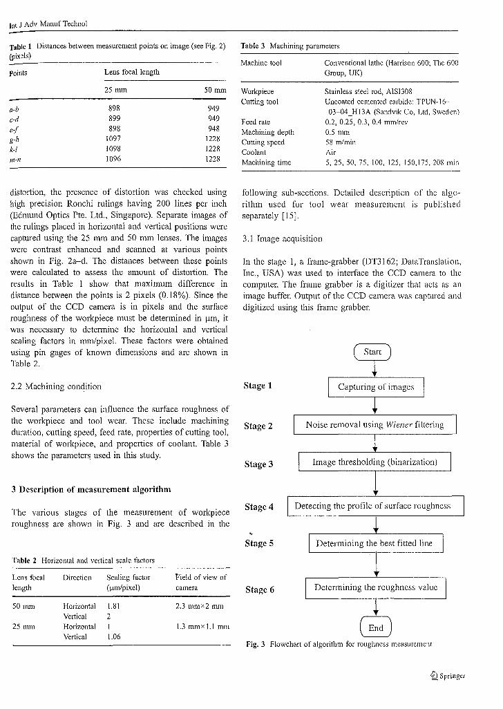
Table 1 Distances between measurement points on image (see Fig. 2)(pixels)

Table 3 Machining parameters

points Lens focal lengthMachine tool Conventional lathe (Han'ison 600; The 600

Group, UK)

a-bc-de{g-h

k-lm-n

25 mm

898899898

109710981096

50mm

949949948

122812281228

WorkpieceCutting tool

Feed rateMachining depthCutting speedCoolantMachining time

Stainless steel rod, AISI308Uncoated cemented carbide: TPUN-16·03-04_H13A (Sandvik Co, Ltd, Sweden)

0.2, 0.25, 0.3, 0.4 mmlrev0.5 mm58 m/min

Air5,25,50,75, 100, 125, 150,175,208 min

3.1 Image acquisition

following sub-sections. Detailed description of the algo­rithm used for tool wear measurement is publishedseparately [IS].

Image thresholding (binarization)

Noise removal using Wiener filtering

Stage 3

Stage 2

Stage 1

In the stage 1, a frame-grabber (DT3162; DataTranslation,Inc., USA) was used to interface the CCD camera to thecomputer. The frame grabber is a digitizer that acts as animage buffer. Output of the CCD camera was captured anddigitized using this frame grabber.

distortion, the presence of distortion was checked usinghigh precision Ronchi rulings having 200 lines per inch(Edmund Optics Pte. Ltd., Singapore). Separate images ofthe rulings placed in horizontal and vertical positions werecaptured using the 25 mm and 50 mm lenses. The imageswere contrast enhanced and scanned at various pointsshown in Fig. 2a-d. The distances between these pointswere calculated to assess the amount of distortion. Theresults in Table I show that maximum difference indistance between the points is 2 pixels (0.18%). Since theoutput of the CCD camera is in pixels and the surfaceroughness of the workpiece must be determined in J.lm, itwas necessary to determine the horizontal and verticalscaling factors in mm/pixel. These factors were obtainedusing pin gages of known dimensions and are shown inTable 2.

Several parameters can influence the surface roughness ofthe workpiece and tool wear. These include machiningduration, cutting speed, feed rate, properties of cutting tool,material of workpiece, and properties of coolant. Table 3shows the parameters used in this study.

3 Description of measurement algorithm

2.2 Machining condition

The various stages of the measurement of workpieceroughness are shown in Fig. 3 and are described in the

Stage 4 Detecting the profile of surface roughness

Stage 5 Determining the best fitted line

Fig. 3 Flowchart of algorithm for roughness measurement

Table 2 Horizontal and vertical scale factors

Lens focal Direction Scaling factor Field of view oflength (Il-m/pixel) camera

50 mm Horizontal 1.81 2.3 mm x 2 mm

Vertical 225 mm Horizontal I 1.3 mm x 1.1 mm

Vertical 1.06

Stage 6 Determining the roughness value

©Springer

Int J Adv Manuf Technol

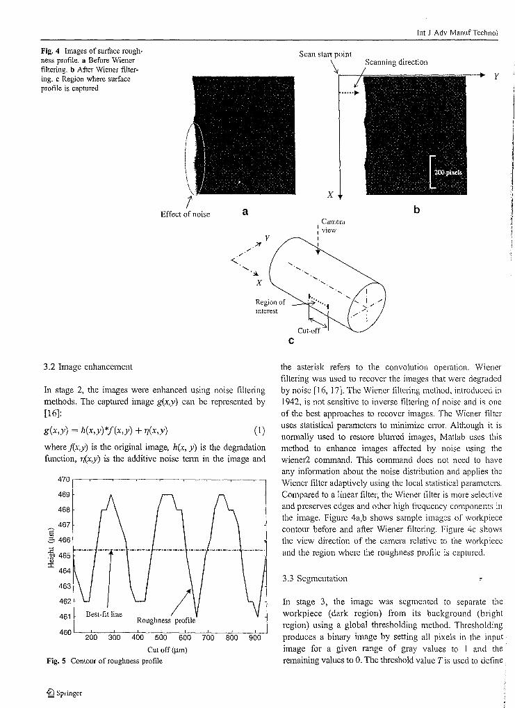
Fig. 4 Images of surface rough­ness profile. a Before Wienerfiltering. b After Wiener filter­ing. c Region where surfaceprotile is captured

Effect of noise

y.?f

/

Scan start point

\

x

CameraI .I viewII

Scanning direction

y

b

Region ofimeresl

3.2 Image enhancement

460 L.--::-'-=-~'-o---:~-::-::-::---=-'-::---=~-~--::-7-=--'200 300 400 500 600 700 800 900

Cut off (I.tm)

Fig. 5 Contour of roughness profile

the asterisk refers to the convolution operation. Wienerfiltering was used to recover the images that were degradedby noise [16, 17]. The Wiener filtering method, introduced in1942, is not sensitive to inverse filtering of noise and is oneof the best approaches to recover images. The Wiener filteruses statistical parameters to minimize error. Although it isnonnally used to restore blU11'ed images, Matlab uses thismethod to enhance images affected by noise using thewiener2 command. This command does not need to haveany infonnation about the noise distribution and applies theWiener filter adaptively using the local statistical parameters.Compared to a linear filter, the Wiener filter is more selectiveand preserves edges and other high frequency components inthe image. Figure 4a,b shows sample images of workpiececontour before and after Wiener filtering. Figure 4c showsthe view direction of the camera relative to the workpieceand the region where the roughness profile is captured.

In stage 3, the image was segmented to separate theworkpiece (dark region) from its background (brightregion) using a global thresholding method. Thresholdingproduces a binary image by setting all pixels in the inputimage for a given range of gray values to 1 and theremaining values to O. The threshold value T is used to define.

3.3 Segmentation

Roughness profileBest-fit line461

463

470 '--"'--~--"----~-~--"'-----'--r---o

469

468

467E.3 466

~Q 465~

464

In stage 2, the images were enhanced using noise filteringmethods. The captured image g(x,y) can be represented by[16]:

g(x,y) = h(x,y)*f(x,y) + 7J(x,y) (1)

where j(x,y) is the original image, hex, y) is the degradationfunction, 7J(x,y) is the additive noise term in the image and

tQ Springer

Int J Adv Manuf Technol

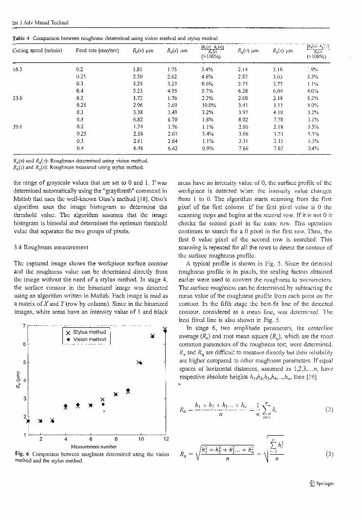
Table 4 Comparison between roughness determined using vision method and stylus method

Cutting speed (m/min) Feed rate (mm/rev) R,,(v) ~m R,,(s) ~mIR"(s)-R"(vll

Rq(v) ~m Rq(s) ~111!R./,) R.,(,·i!

R"(s) R.,(s)(xIOO%) (xIOO%)

16.3 0.2 1.81 1.75 3.4% 2.14 2.10 1.9%0.25 2.50 2.62 4.6% 2.87 3.03 5.3%0.3 3.25 3.23 0.6% 3.73 3.77 1.1%0.4 5.23 4.95 5.7% 6.28 6.04 4.0'Yo

23.8 0.2 1.72 1.76 2.3% 2.00 2.18 8.3%0.25 2.96 2.69 10.0% 3.41 3.13 9.0'Yo0.3 3.38 3.49 3.2% 3.97 4.10 3.2%0.4 6.82 6.70 1.8% 8.02 7.78 3.1%

39.6 0.2 1.74 1.76 1.1% 2.06 2.18 5.5%0.25 2.58 2.67 3.4% 3.06 3.23 5.3%0.3 2.61 2.64 1.1% 3.11 3.15 1.3%

0.4 6.48 6.42 0.9% 7.66 7.63 0.4%

K,(v) and Rq(v): Roughness determined using vision method.Rq(s) and R,is): Roughness measured using stylus method.

6

the range of grayscale values that are set to 0 and 1. Twasdetermined automaticaily using the "graythresh" command inMatlab that uses the well-known Otsu's method [18]. Otsu'salgorithm uses the image histogram to detennine thethreshold value. The algorithm assumes that the imagehistogram is bimodal and detennines the optimum thresholdvalue that separates the two groups of pixels.

3.4 Roughness measurement

The captured image shows the workpiece surface contourand the roughness value can be determined directly fromthe image without the need of a stylus method. In stage 4,the surface contour in the binarized image was detectedusing an algorithm written in Matlab. Each image is read asa matrix of X and Y (row by column). Since in the binarizedimages, white areas have an intensity value of 1 and black

7r--,---;:=====:::::;-r---~--~

IX Stylus method I• Vision method

5

areas have an intensity value of 0, the surface profile of theworkpiece is detected when the intensity value changesfrom I to O. The algorithm starts scanning from the firstpixel of the first column. If the first pixel value is 0 thcscanning stops and begins at the second row. If it is not 0 itchecks the second pixel in the same row. This operationcontinues to search for a 0 pixel in the first row. Then, thefirst 0 value pixel of the second row is searched. Thisscanning is repeated for all the rows to detect the contour ofthe surface roughness profile.

A typical profile is shown in Fig. 5. Since the detectedroughness profile is in pixels, the scaling factors obtainedearlier were used to convert the roughness to micrometers.The surface roughness can be detemlined by subtracting themean value of the roughness profile from each point on thecontour. In the fifth stage the best-fit line of the detectedcontour, considered as a mean line, was determined. Thebest fitted line is also shown in Fig. 5.

In stage 6, two amplitude parameters, the centerlineaverage (Ra) and root mean square (Rq), which are the mostcommon parameters of the roughness test, were determined.Ra and Rq are difficult to measure directly but their reliabilityare higher compared to other roughness parameters. If equalspaces of horizontal distances, assumed as 1,2,3, .. .n, haverespective absolute heights h\,h2,h3,h4 , ... ,h", then [19]

3

2(2)

Measurement number

Fig. 6 Comparison between roughness determined using the visionmethod and the stylus method

2 4 6 8 10 12

hi + h~ + h~ ... + h~

n

11

I:,hli~"

n(3)

%) Springer

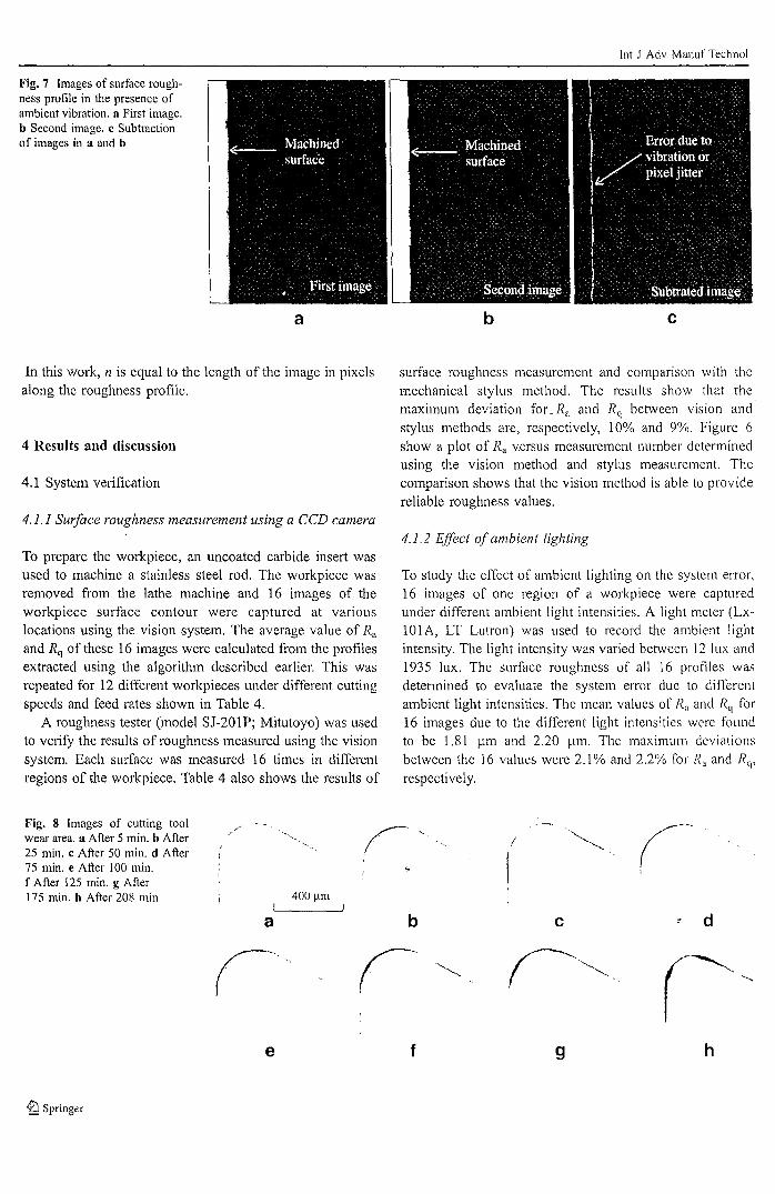
Fig. 7 Images of surface rough­ness profile in the presence ofambient vibration. a First image.b Second image. c Subtractionof images in a and b

Int J Adv ManuI' Technol

a b c

In this work, n is equal to the length of the image in pixelsalong the roughness profile.

4 Results and discussion

4.1 System verification

4.1.1 Surface roughness measurement using a CCD camera

To prepare the workpiece, an uncoated carbide insert wasused to machine a stainless steel rod. The workpiece wasremoved from the lathe machine and 16 images of theworkpiece surface contour were captured at variouslocations using the vision system. The average value of Ra

and Rq of these 16 images were calculated from the profilesextracted using the algorithm described earlier. This wasrepeated for 12 different workpieces under different cuttingspeeds and feed rates shown in Table 4.

A roughness tester (model SJ-201P; Mitutoyo) was usedto verify the results of roughness measured using the visionsystem. Each surface was measured 16 times in differentregions of the workpiece. Table 4 also shows the results of

surface roughness measurement and comparison with themechanical stylus method. The results show that themaximum deviation fOL Ra and Rq between vision andstylus methods are, respectively, 10% and 9%. Figure 6show a plot of Ra v.ersus measurement number detetminedusing the vision method and stylus measurement. Thecomparison shows that the vision method is able to providereliable roughness values.

4.1.2 Effect of ambient lighting

To study the effect of ambient lighting on the system error,16 images of one region of a workpiece were capturedunder different ambient light intensities. A light meter (Lx­lOlA, LT Lutron) was used to record the ambient lightintensity. The light intensity was varied between 12 lux and1935 lux. The surface roughness of all 16 profiles wasdetetmined to evaluate the system error due to differentambient light intensities. The mean values of Ra and Rq for16 images due to the different light intensities were foundto be 1.81 }-Lm and 2.20 }-Lm. The maximum deviationsbetween the 16 values were 2.1 % and 2.2% for Ra and R,prespectively.

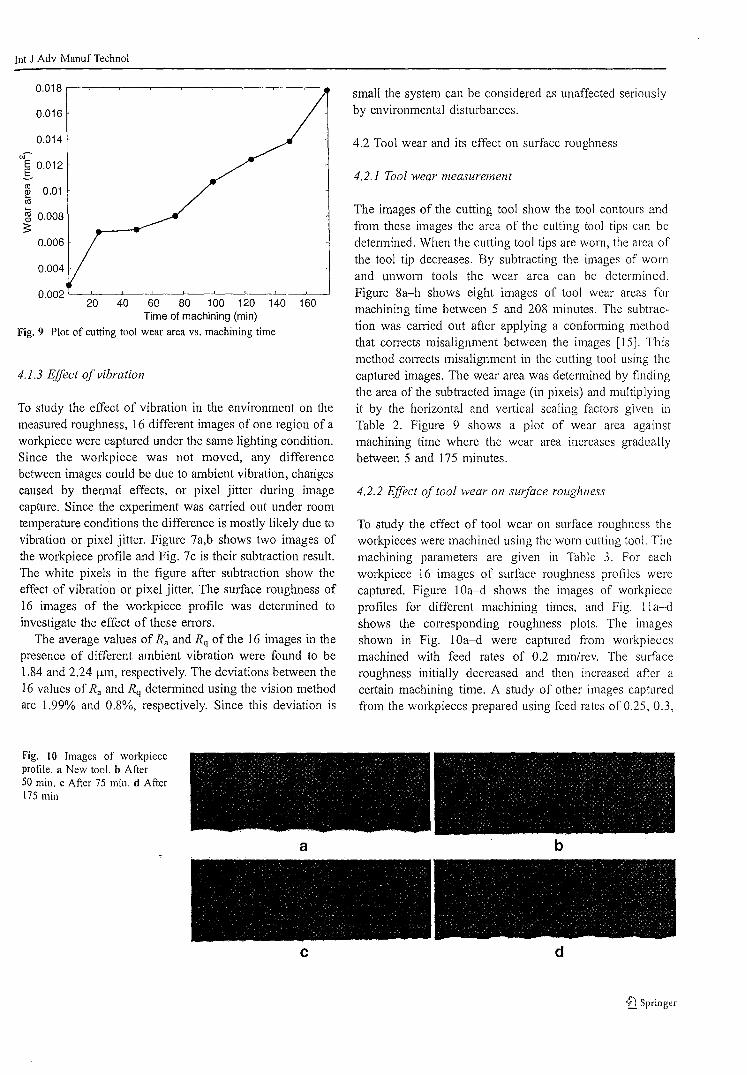
Fig. 8 Images of cutting toolwear area. a After 5 min. b After25 min. c After 50 min. dAfter75 min. e After 100 min.f After 125 min. g After175 min. h After 208 min

a

400 )lm

b

!

r

c d

1d Springer

e f 9 h

Int J Adv Manuf Technol

4.1.3 Ejfect of vibration

4.2.2 Effect of tool wear on surface roughness

To study the effect of tool wear on surface roughness theworkpieces were machined using the worn cutting tool. Themachining parameters are given in Table 3. For eachworkpiece 16 images of surface roughness profiles werecaptured. Figure 10a-d shows the images of workpieceprofiles for different machining times. and Fig. II a-dshows the corresponding roughness plots. The imagesshown in Fig. 10a-d were captured from workpiecesmachined with feed rates of 0.2 mm/rev. The surfaceroughness initially decreased and then increased after acertain machining time. A study of other images capturedfrom the workpieces prepared using feed rates of 0.25,0.3,

4.2.1 Tool wear measurement

The images of the cutting tool show the tool contours andfrom these images the area of the cutting tool tips can bedetermined. When the cutting tool tips are worn, the area ofthe tool tip decreases. By subtracting the images of WOl11

and unworn tools the wear area can be determined.Figure 8a-h shows eight images of tool wear areas formachining time between 5 and 208 minutes. The subtrac­tion was carried out after applying a conforming methodthat con'ects misalignment between the images [15]. Thismethod con'ects misalignment in the cutting tool using thecaptured images. The wear area was detennined by findingthe area of the subtracted image (in pixels) and multiplyingit by the horizontal and vertical scaling factors given inTable 2. Figure 9 shows a plot of wear area againstmachining time where the wear area increases graduallybetween 5 and 175 minutes,

4.2 Tool wear and its effect on surface roughness

small the system can be considered as unaffected seriouslyby environmental disturbances.

160

0.006

0.016

0.004

To study the effect of vibration in the environment on themeasured roughness, 16 different images of one region of aworkpiece were captured under the same lighting condition.Since the workpiece was not moved, any differencebetween images could be due to ambient vibration, changescaused by thennal effects, or pixel jitter during imagecapture. Since the experiment was carried out under roomtemperature conditions the difference is mostly likely due tovibration or pixel jitter. Figure 7a,b shows two images ofthe workpiece profile and Fig. 7c is their subtraction result.The white pixels in the figure after subtraction show theeffect of vibration or pixel jitter. The surface roughness of16 images of the workpiece profile was determined toinvestigate the effect of these errors.

The average values of Ra and Rq of the 16 images in thepresence of different ambient vibration were found to be1.84 and 2.24 J-lm, respectively. The deviations between the16 values of Ra and Rq detennined using the vision methodare 1.99% and 0.8%, respectively. Since this deviation is

0.002 L---L_--'-_----'-_---'_----''-_'--_-'----_-'------'

20 40 60 80 100 120 140Time of machining (min)

Fig. 9 Plot of cutting tool wear area vs. machining time

0.014

1. 0.012

~ 0.01<1l

m0.008~

Fig. 10 Images of workpieceprofile. a New tool. b After50 min. c After 75 min. dAfter175 min

a b

c d

id Springer

In! J Adv ManuI' Technol

570 515

510

560 505

500

E 550 E 4956 615 15 490oll Oll

'(i) 540 '0) 485::r::: ::r:

480

530 475

470

520 4650 200 400 600 800 1000 0 200 400 600 800 1000

Cut off (J..Lm) Cut off (J..Lm)

a b

450 530

440 520

E 430 E 510::l.. 6.'-'~

15.cOll Oll

'0) 420 '0) 500::r: ::r:

410 490

400 480a 200 400 600 800 1000 0 200 400 600 800 1000

Cut off (J..Lm) Cut off (J..Lm)

C dFig. 11 Roughness profiles of workpiece. a New tool. b After 50 min. c After 75 min. dAfter 175 min

-*- Feed rate", 0.2 mm/rev

-+- Feed rate", 0.25 mmlrev-II- Feed rate", 0.3 mmlrev

--+- Feed rate", 0.4 mm/rev10

12

OL---'-_-.Jl-_-L.-_---'--_----'--_--'-_-.J__L----.-J

20 40 60 80 100 120 140 160

Machining time (min)

Fig. 12 Effect of feed rate and machining time on Ra

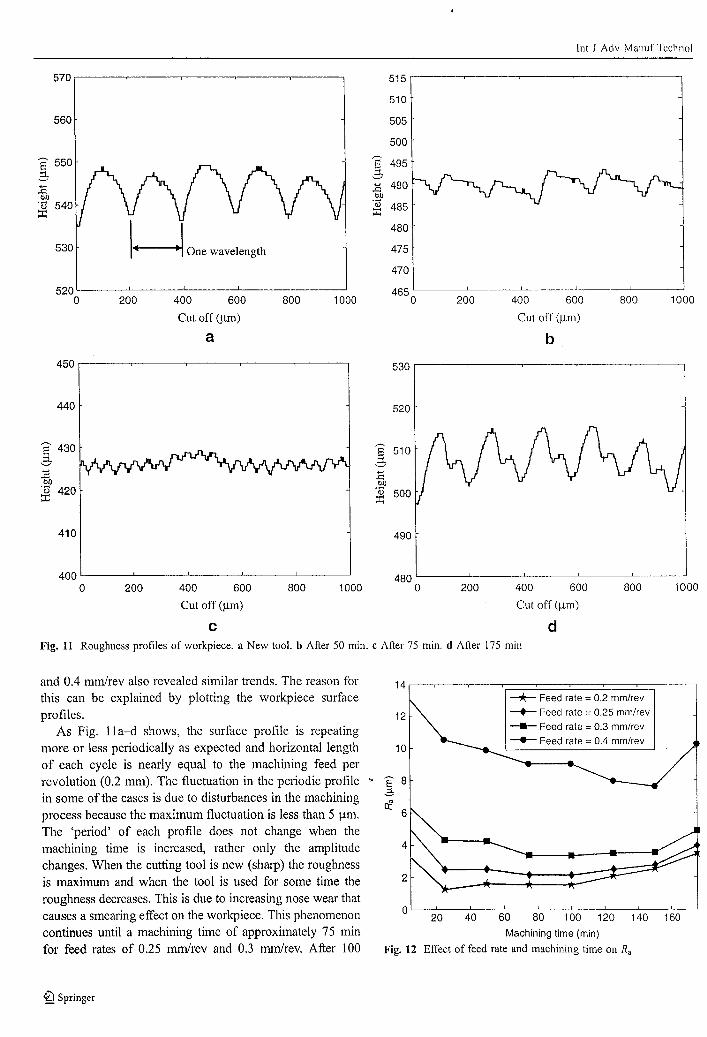
and 0.4 mm/rev also revealed similar trends. The reason forthis can be explained by plotting the workpiece surfaceprofiles.

As Fig. 11 a-d shows, the surface profile is repeatingmore or less periodically as expected and horizontal lengthof each cycle is nearly equal to the machining feed perrevolution (0.2 mm). The fluctuation in the periodic profile '>

in some of the cases is due to disturbances in the machiningprocess because the maximum fluctuation is less than 5 J..Lm.The 'period' of each profile does not change when themachining time is increased, rather only the amplitudechanges. When the cutting tool is new (sharp) the roughnessis maximum and when the tool is used for some time theroughness decreases. This is due to increasing nose wear thatcauses a smearing effect on the workpiece. This phenomenoncontinues until a machining time of approximately 75 minfor feed rates of 0.25 mm/rev and 0.3 mm/rev. After 100

id Springer

lnt J Adv Manuf Technol

minutes of machining time the roughness increases andcontinues to increase until the cutting tool breaks or is badlywom (175 min). Figure 12 shows the variation of surfaceroughness with machining time determined using themachine vision system. When the feed rate is higher, theroughness value is greater at any machining time.

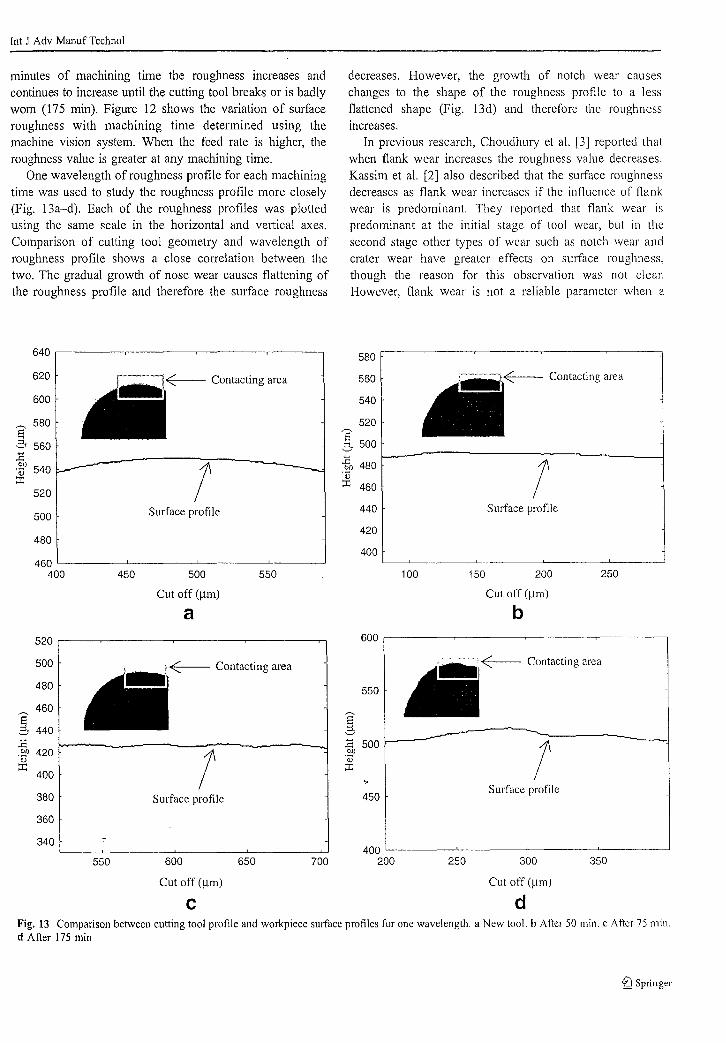
One wavelength of roughness profile for each machiningtime was used to study the roughness profile more closely(Fig. 13a-d). Each of the roughness profiles was plottedusing the same scale in the horizontal and vertical axes.Comparison of cutting tool geometry and wavelength ofroughness profile shows a close correlation between thetwo. The gradual growth of nose wear causes flattening ofthe roughness profile and therefore the surface roughness

decreases. However, the growth of notch wear causeschanges to the shape of the roughness profile to a lessflattened shape (Fig. 13d) and therefore the roughnessincreases.

In previous research, Choudhury et al. [3] reported thatwhen flank wear increases the roughness value decreases.Kassim et al. [2] also described that the surface roughnessdecreases as flank wear increases if the influence of flankwear is predominant. They reported that flank wcar ispredominant at the initial stage of tool wear, but in thesecond stage other types of wear such as notch wear andcrater wear have greater effects on surface roughness,though the reason for this observation was not clear.However, flank wear is not a reliable parameter when a

640 ,------,------,------,--------,

250

!Surface profile

150 200

Cut off (~Lm)

b

100

580

560

540

520s~ 500

\.-.------------~----:--~-~~____1

fn 480'v::c 460

440

420

400

-------

550500

Cut off (j..lm)

a

!Surface profile

450

r"~'-~~J-E-- Contacting area

.-460 '-- --1. -'- -L.-__---'

400

480

500

520

600

620

5808'~ 560

!

600 r----~----~---~----,

350

---'--'---~--......._~I

!

300

Cut off (!Jm)

d

Surface profile

250

ii" _E__ Contacting area

•400 '-- '-- .L- -'-- .._

200

550

~a~.c 500bn'v::c

.,.

450

700650600

Cut off (j..lm)

C

Surface profile

550

520

500

480

460E~ 440.c.~n 420OJ

::c 400

380

360

340

Fig. 13 Comparison between cutting tool profile and workpiece surface profiles for one wavelength, a New tool. b After 50 min. c After 75 min.dAfter 175 min

~ Springer

surface roughness requirement has to be met [19, 20]. In asimilar study, Pavel et a1. [13] reported that when the outputof a machining process is continuous chip the roughnessvalue increased with machining time. When the chip is notcontinuous the roughness value decreased with machiningtime. When notch wear is negligible the surface roughnessdecreases with flank wear, and when notch wear increasesthe roughness value increases. This was, however, notconfinned experimentally in their paper. The results of ourstudy show that increasing flank wear flattens the tool nosearea and this decreases the surface roughness of theworkpiece. However, increasing notch wear after 75 minutesof machining time increases the roughness value. Themachine vision system developed in this work can beextended to further study the effect ofnose wear on workpiecesurface roughness under other machining conditions, such asdifferent workpiece materials and cutting speeds.

5 Conclusion

The noncontact method using machine vision proposed inthis work and in previous work [15] enables the measure­ment of both cutting tool nose wear area and surfaceroughness of turned parts using the same setup. Analgorithm that employs Wiener filtering and simple thresh­olding on backlit images reduces errors caused by theenvironmental factors such as ambient lighting and vibra­tion. A comparative study using the stylus method ofroughness measurement showed that the maximum devia­tion in roughness value measured using the proposedsystem is about 10%. A study of 2D tool wear area usingthe system developed shows that increasing the feed rateincreases the smface roughness if other machining param­eters are not changed. Also, the results show that increasingthe machining time of the tool decreases the surfaceroughness in the first stage of machining due to increasein nose wear. However, in the second stage of machining(after 75 minutes), the roughness value increases due to theeffect of growing notch wear.

The surface profiles of the workpiece show thatroughness is periodic as expected, and this was clearlyvisible at different machining times. A close correlation was­found to exist between the shape of the wear area of thecutting tool and the roughness profile. The system andmeasurement algorithm developed can be applied withinthe workshop environment for the in-cycle monitoring oftool wear and workpiece surface roughness.

~ Springer

Int J Adv ManuI' Technol

Acknowledgement The authors wish to thank Universiti SainsMalaysia for the short-term grant that enabled this study to be calTied out.

References

I. Kurada S, Bradley C (1997) A review of machine vision sensorsfor tool condition monitoring. Comput Ind 34:55-72

2. Kassim AA, Mian Z, Mannan MA (2004) Connectivity orientedfast Hough transform for tool wear monitoring. Pattem Recogn37: 1925-1933

3. Choudhury SK, Bartarya G (2003) Role of temperature andsurface finish in predicting tool wear using neural network anddesign of experiments. Int J Mach Tools ManuI' 43:747-753

4. Sortino M (2003) Application of statistical filtering for opticaldetection of tool wear. Int J Mach Tools ManuI' 43:493-497

5. Pfeifer T, Wiegers L (2000) Reliable tool wear monitoring byoptimized image and illumination control in machine vision.Measurement 28:209-218

6. Lanzetta M (200 I) A new flexible high-resolution vision sensorfor tool condition monitoring. J Mater Process Technol 119:7382

7. Yang MY, Kwon OD (1996) Crater wear measurement usingcomputer vision and automatic focusing. J Mater Process Technol58:362-367

8. Wang WH, Hong GS, Wong YS (2006) Flank wear measurementby a threshold independent method with sub-pixel accuracy. 1m .JMach Tool Manu 46(2): 199-207

9. Kurada S, Bradley C (1997) A machine vision system for toolwear assessment. Tribology Int 30(4):294-304

10. Jurkovic J, Korosec M, Kopac J (2005) New approach in toolwear measuring technique using CCD vision system. Int J MachTools Manu 45:1023-1030

II. Dawson TG, Kurfess TR (2005) Quantification of tool wear usingwhite light intelferometry and three-dimensional computationalmelt·ology. Int .J Mach Tool Manu 45:591--596

12. Mannan MA, Kassim AA, Jing M (2000) Application of imageand sound analysis techniques to monitor the condition of cuttingtools. Pattern Recogn Lett 21 :969.. 979

13. Pavel R, Marinescu J, Deis M, Pillar J (2005) Effect of tool wearon surface finish for a case of continuous and interrupted hardturning. J Mater Process Technol 170:341349

14. Tamizharasan T, Selvaraj T, Noorul Haq A (2006) Analysis of toolwear and surface finish in hard turning. Int J Adv ManufTechnol28:671-679

IS. Shahabi HH, Ratnam MM (2007) On-line monitoring of tool wearin turning operation in the presence of tool misalignment. Int JAdv ManuI' Tech. DOl 10.1007/s00170-007-1119-4

16. Gonzalez RC, Woods RE, Eddins SL (2004) Digital imageprocessing using Matlab. Pearson-Prentice Hall, New Jersey

17. Lim JS (1990) Two-dimensional signal and image processing.Prentice Hall, Englewood Cliffs, NJ, pp 536-540

18. Otsu N (1979) A threshold selection method tl'om gray-levelhistograms. IEEE Trans Syst Man Cybem 9( 1):62-66

19. Gayler JFW, Shotbolt CR (1990) Metrology for engineers.Cassell, London

20. Kwon Y, Fischer GW (2003) A novel approach to quantifying toolwear and tool life measurements for optimal tool management. IntJ Mach Tool Manu 43:359-368

lnt J Adv Manuf Technol

DOl 10.1007/sOO 170-007-1119-4

On-line monitoring of tool wear in turning operationin the presence of tool misalignment

H. H. Shahabi . M. M. Ratnam

Received: 3 January 2007/Accepted: 4 June 2007C¢) Springer-Verlag London Limited 2007

Abstract A VISIon system using high-resolution CCDcamera and back-light was developed for the on-linemeasurement of nose wear of cutting tool inserts. Initialstudy showed that the system is sensitive to several factors inthe work environment such as misalignment of cutting tool,presence of micro-dust particles, vibration and intensityvariation of ambient light. An algorithm using Wienerfiltering, median filtering, morphological operations andthresholding was developed to decrease the system errorcaused by these factors. A conforming method was used toovercome misalignment of the tool insert during offline andon-line measurement. The algOlithm, combined with asubtraction method, was applied to measure the nose weararea of the inserts under different machining conditions.

Keywords Machine vision· Tool wear· Wiener filtering·Confooning

1 Introduction

Tool wear during machining operations is known to changethe geometry of the cutting tool, thus increasing cuttingforce, affecting surface finish and decreasing dimensionalaccuracy of the work piece. Monitoring of tool wear duringmachining is important to detect problems in the cuttingprocess, assess stability of machining, control surface finishof product and avoid damage to the machine tool itself.

H. H. Shahabi . M. M. Ratnam (C>::<:i)School of Mechanical Engineering, Engineering Campus,Universiti Sains Malaysia,14300 Nibong Tebal, Malaysiae-mail: nunaran@eng.usm.my

Thus, tool wear has been studied extensively as a significantresearch area in manufacturing in the past [1-18].

Most of the previous work in tool wear monitoringconcerns the measurement of crater wear and flank wearusing 2-D and 3-D methods. Crater wear occurs due to thecontact of chips with the rake face, while flank wear is due tothe rubbing of the work piece with the cutting tool.Measurement of flank and crater wear has been carried outmostly using offline methods due to the nature of the weararea and difficulty in implementing the instruments for on-linemeasurement. Investigation into the possibility of measuringnose wear for on-line (in-process) tool wear monitoring islimited. Lanzetta [6] measured nose wear offline using a toolfixture and found that the use of profile projection issufficiently accurate to measure the wear area. A similartechnique using back-lighting has been used for extractingthe lost material of a cutting tool from its 2-D profile [7].

Tool wear measurement methods can generally bedivided into indirect and direct methods. Examples ofindirect methods include acoustic emission, tool tiptemperature monitoring, vibration signatures (accelerationsignals), cutting force monitoring, stress/strain analysis andspindle motor current monitoring. In these methods theoptimized signal of the machining process is compared tothe live signals. Wl1en a live signal deviates from thc.,.optimized signal, -the system notifies the need to change thecutting tool. The acoustic emission and cutting forcemeasurement methods have been employed to monitor theeutting process in industries [8]. The main advantage ofindirect methods is their ability to be applied for on-linetool wear monitoring. Their implementation is, however,not easy due to inadequate knowledge on the effect of toolwear on the signals produced.

Machine vision can be used for directly measuring toolwear because different foons and geometries can be readily

~ Springer

lnt J Adv Manuf Technol

CCD cameraFrame grabber

2.2 Machining condition

Various parameters can influence the wear rate of thecutting tool, such as machining time, cutting speed, feedrate, tool material, work piece material and type of coolant.Table 1 shows the parameters used to shape the wear area inthis study. The machine used was a conventional lathemachine (Model: Pinocho S901200 (Italy)) and the workpiece was low-carbon steel bars of 45 mm diameter. The

.4

() , ///,:~Light source " ", " " , " Cutting tool

... "", .... , ... .::i,.. ),' I ,','

....... ", ~ 'II lIJx I insclt.. :::l.....::i... '1:,' / '1'-

................ ';' ... ,"- ...:.. /..... ;/~./'~...............Reflcetor

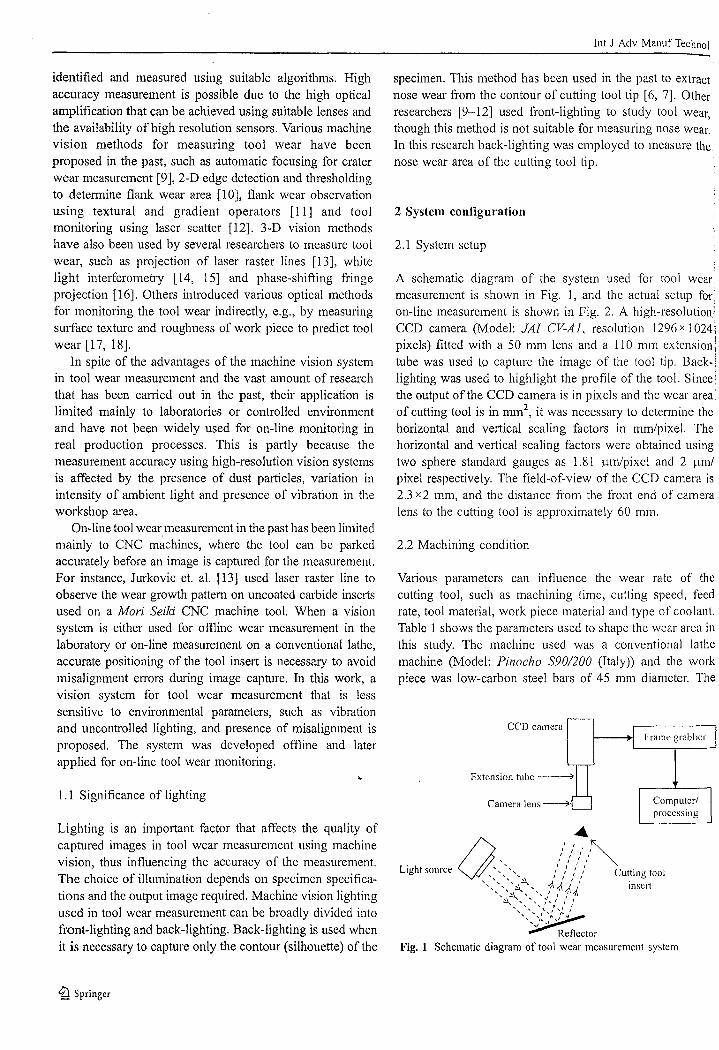
Fig. 1 Schematic diagram of tool wear measurement system

A schematic diagram of the system used for tool wear;measurement is shown in Fig. 1, and the actual setup forion-line measurement is shown in Fig. 2. A high-resolution!CCD camera (Model: JA! CV-Al, resolution 1296x 1024;pixels) fitted with a 50 mm lens and a 110 mm extension:tube was used to capture the image of the tool tip. Back-:lighting was used to highlight the profile of the tool. Since)the output of the CCD camera is in pixels and the wear areaof cutting tool is in mm2

, it was necessary to detennine thehorizontal and vertical scaling factors in mm/pixel. Thehorizontal and vertical scaling factors were obtained usingtwo sphere standard gauges as 1.81 I-un/pixel and 2 I-lm/pixel respectively. The field-of-view of the CCD camera is2.3 x2 mm, and the distance from the front end of cameralens to the cutting tool is approximately 60 mm.

2.1 System setup

2 System configuration

specimen. This method has been used in the past to extractnose wear from the contour of cutting tool tip [6, 7]. Otherresearchers [9-12] used front-lighting to study tool wear,though this method is not suitable for measuring nose wear.In this research back-lighting was employed to measure thenose wear area of the cutting tool tip.

Lighting is an important factor that affects the quality ofcaptured images in tool wear measurement using machinevision, thus influencing the accuracy of the measurement.The choice of illumination depends on specimen specifica­tions and the output image required. Machine vision lightingused in tool wear measurement can be broadly divided intofront-lighting and back-lighting. Back-lighting is used whenit is necessary to capture only the contour (silhouette) of the

1.1 Significance of lighting

identified and measured using suitable algorithms. Highaccuracy measurement is possible due to the high opticalamplification that can be achieved using suitable lenses andthe availability of high resolution sensors. Various machinevision methods for measuring tool wear have beenproposed in the past, such as automatic focusing for craterwear measurement [9], 2-D edge detection and thresholdingto detennine flank wear area [10], flank wear observationusing textural and gradient operators [II] and toolmonitoring using laser scatter [12]. 3-D vision methodshave also been used by several researchers to measure toolwear, such as projection of laser raster lines [13], whitelight interferometry [14, 15] and phase-shifting fringeprojection [16]. Others introduced various optical methodsfor monitoring the tool wear indirectly, e.g., by measuringsurface texture and roughness of work piece to predict toolwear [17, 18].

In spite of the advantages of the machine vision systemin tool wear measurement and the vast amount of researchthat has been carried out in the past, their application islimited mainly to laboratories or controlled environmentand have not been widely used for on-line monitoring inreal production processes. This is partly because themeasurement accuracy using high-resolution vision systemsis affected by the presence of dust particles, variation inintensity of ambient light and presence of vibration in theworkshop area.

On-line tool wearmeasurement in the past has been limitedmainly to CNC machines, where the tool can be parkedaccurately before an image is captured for the measurement.For instance, Jurkovic et. al. [13] used laser raster line toobserve the wear growth pattern on uncoated carbide insertsused on a Mori Seiki CNC machine tool. When a visionsystem is either used for offline wear measurement in thelaboratOly or on-line measurement on a conventional lathe,accurate positioning of the tool insert is necessary to avoidmisalignment errors during image capture. In this work, avision system for tool wear measurement that is lesssensitive to environmental parameters, such as vibrationand uncontrolled lighting, and presence of misalignment isproposed. The system was developed offline and laterapplied for on-line tool wear monitoring.

~ Springer

Int J Adv Manuf Technol

3.2 Image enhancement

across the image, whereby a sharp image produced maxi­mum intensity gradient between the btight and dark regions.

In Stage 2, the images were enhanced using noise filteringmethods. The captured image g(t, y) can be represented by:

( 1)

where j(x,y) is the original image, and TJ(t,y) is the noiseterm in the image.

Median filtering and Wiener filtering were used torecover the images of cutting tools that were degraded bynoise. Median filtering is a method used to remove impulsenoise without bluning the image. This method replaces thecunent pixel by the median of neighborhood pixels within amask. Compared to other filtering methods, medianfiltering maintains the edge details in the Oliginal imagewhile reducing noise [19]. The Wiener filtering method isan early method used to recover images comlpted by noise[20]. This method is one of the best approaches to recoverthe images and it is not sensitive to inverse filter of noise.

Figure 4 (a)--(c) show the effect of applying medianfiltering on the intensity profile across the tool insert.Figure 4 (b) shows the intensity profile after median filteringusing a 3 x3 window and Fig. 4 (c) shows the optimumintensity profile obtained using a lOx 10 window. Sincedifferent filter mask sizes produced different results, a totalof 10 masks ranging from 2 x2 to 11 x 11 were used todetermine the optimum mask size. Figure 4 (d) shows theeffect of using Wiener filtering on the intensity profile.Figure 5 shows the wear area of the cutting tool inse11 beforefiltering (Fig. 5 (a)), after applying median filteling (Fig. 5 (b»and after applying Wiener filtering (Fig. 5 (C». Although theresults after applying median and Wiener filtering look almostalike, there is a finite difference in the wear areas.

g(x,y) = f(x,y) + 1](x,y)

In Stage 1, a frame-grabber (data translation-DT3162) wasused to interface the CCD camera to the computer. Output ofthe camera was captured using the frame grabber. In thisstudy, it is important to ensure sharpness of image capturedbecause blurring decreases the accuracy of measurement. Thesharpness of image was ensured using the intensity profiles

3.1 Image acquisition

The various stages involved in the measurement of nosewear area are shown in Fig. 3, and are described below.

3 Wear measurement algorithm

cutting tools were uncoated carbide inserts manufactured bySandvik Co. Ltd. (Sweden). Three cutting speeds and fourmachining durations, i.e., 10 min, 20 min, 30 min and40 min, were used to monitor the growth of wear area ofthe cutting tool insert.

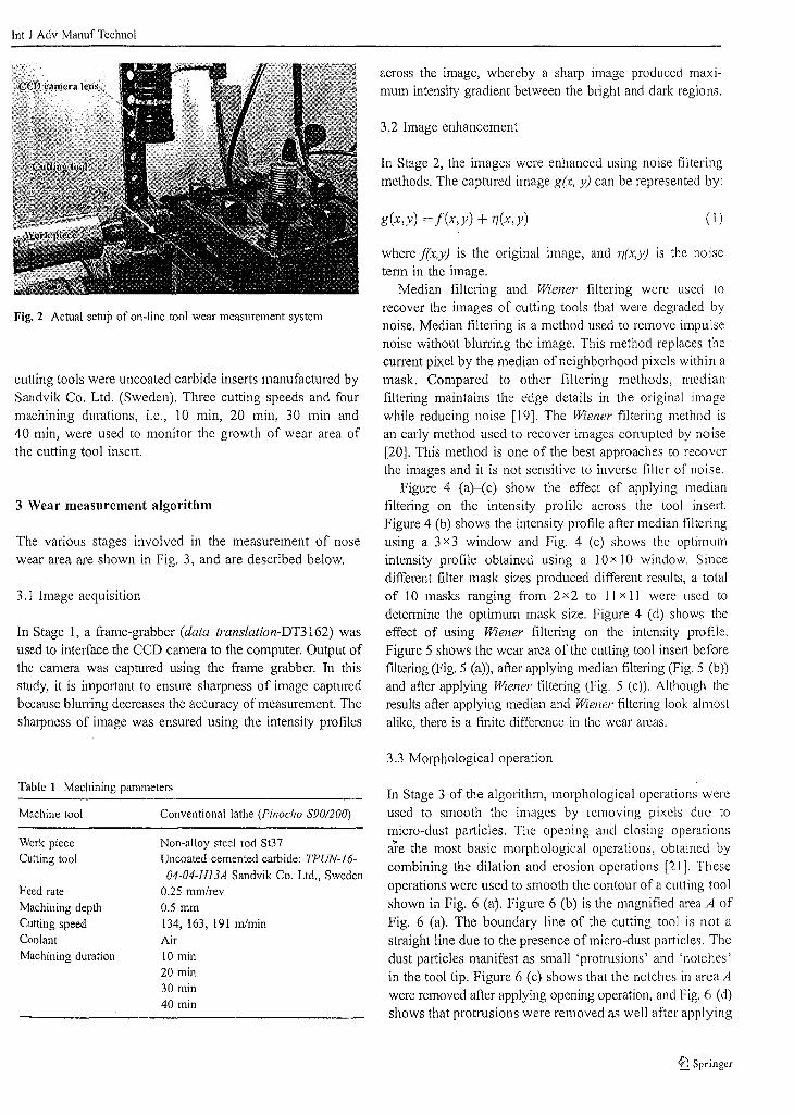
Fig. 2 Actual setup of on-line tool wear measurement system

3.3 Morphological operation

Table 1 Machining parameters

Machine tool

Work pieceCutting tool

Feed rate

Machining depth

Cutting speed

Coolant

Machining duration

Conventional lathe (Pinocho S90/200)

Non-alloy steel rod St37Uncoated cemented carbide: TPUN-16-

04-04-Hl3A Sandvik Co. Ltd., Sweden

0.25 mm/rev

0.5 mm

134, 163, 191 m/min

Air

10 min

20 min30 min

40 min

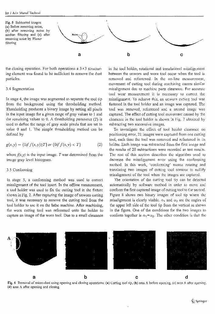
In Stage 3 of the algorithm, morphological operations wereused to smooth the images by removing pixels due tomicro-dust particles. The opening and closing operationsare the most basic morphological operations, obtained bycombining the dilation and erosion operations [21]. Theseoperations were used to smooth the contour of a cutting toolshown in Fig. 6 (aj. Figure 6 (b) is the magnified area A ofFig. 6 (a). The boundary line of the cutting tool is not astraight line due to the presence of micro-dust particles. Thedust particles manifest as small 'protrusions' and 'notches'in the tool tip. Figure 6 (c) shows that the notches in area Awere removed after applying opening operation, and Fig. 6 (d)shows that protrusions were removed as well after applying

©Springer

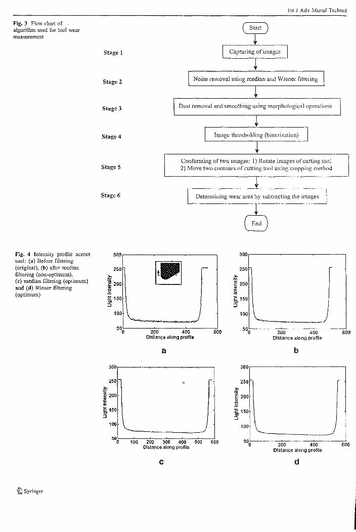
Fig. 3 Flow chart ofalgorithm used for tool wearmeasurement

Stage 1

Stage 2

Stage 3

Stage 4

Stage 5

Stage 6

lnt J Adv Manuf Technol

I Capturing of images I~

INoise removal using median and Wiener filtering I~

I Dust removal and smoothing using morphological operations I~

I Image thresholding (binarization) I~

Conforming of two images: 1) Rotate images of cutting tool2) Move two contours of cutting tool using cropping method

...

Determining wear area by subtracting the images

Fig. 4 Intensity profile acrosstooI: (a) Before fit tering(original), (b) after medianfiltering (non-optimum),(c) median filtering (optimum)and (d) Wiener filtering(optimum)

300r----.,....----...----~

25.0

100

500L..-.---2-'0...0----4-"0-0-----'600

DIStance along profile

a

30ilr--~-~-~--~-~--,

250~-

ell·

i 200

~150::;

300.-----~---~---__.

250

,C.~ 200<I>

£;~ 150::J

100

500L..-.----20.L.O---~4~OO--------'600

Distance along profile

b

300r----~---~---__,

250

~

~·200<I>

£;~ 150:::;

100 100

~ Springer

500~-1~O-=-0--=2~OO:---3:-00'"='O--:4~OO:---5:-'Oc::-0--:-l600

Distance along profile

c

500L-----=-20....,O,-------:-40....,0,---------::-:600

Distance along profile

d

Int J Adv Manuf Technol

Fig. 5 Subtracted images:(a) Before removing noise,(b) after removing noise bymedian filtering and (c) afterremoving noise by Wienerfiltering

a b c

3.5 COnfot111ing

3.4 Segmentation

where f(x,y) is the input image. Twas detennined from theimage gray level histogram.

the closing operation. For both operations a 3 x3 structur­ing element was found to be sufficient to remove the dustparticles.

in the tool holder, rotational and translational misalignmentbetween the unworn and worn tool occur when the tool isremoved and refastened. In the on-line measurement,movement of cutting tool during machining causes similarmisaligmnent due to machine parts clearance. For accuratetool wear measurement it is necessary to COITect themisalignment. To achieve this, an unworn cutting tool wasfastened in the tool holder and an image was captured. Thetool was removed, refastened and a second image wascaptured. The effect of cutting tool movement caused by theclearance in the tool holder is shown in Fig. 7 obtained bysubtracting two successive images.

To investigate the effect of tool holder clearance onpositioning error, 21 images were captured from one cuttingtool, each time the tool was removed and refastened in itsholder. Each image was subtracted from the first image andthe results of 20 subtractions were recorded as test results.The rest of this section describes the algorithm used todecrease the misalignment elTor using the confonningmethod. In this work, 'conforn1ing' means rotating andtranslating two images of cutting tool contour to nullifymisalignment of the tool when the images are captured.

The orientation of the cutting tool tip can be detectedautomatically by software method in order to move andconfonn the first caphlred image of cutting tool to the second.Figure 8 shows two binary images of tool tip where themisalignment is clearly visible. 0:1 and 0:2 are the angles ofthe upper left side of the tool tip from the vertical as shownin the figure. One of the conditions for the two images toconform together is 0:1 =n2. The other condition is that the

(2)g(x,y) = {1!ff(x,Y)2:T}or{Oi[ f(x,y) < T}

In stage 5, a confonning method was used to correctmisalignment of the tool insert. In the offline measurement,a tool holder was used to fix the cutting tool in the fixhtreshown in Fig. 2. After capturing the image of unworn cuttingtool, it was necessary to remove the cutting tool from thetool holder to use it on the lathe machine. After machining,the worn cutting tool was refastened onto the holder tocapture an image of the worn tool. Due to a small clearance

In stage 4, the image was segmented to separate the tool tipfrom the background using the thresholding method.Thresholding produces a binary image by setting all pixelsin the input image for a given range of gray values to 1 andthe remaining values to O. A thresholding parameter (T) isused to define the range of gray scale pixels that are set tovalue 0 and 1. The simple thresholding method can bedefined by

A

a b c dFig. 6 Removal of micro-dust using opening and closing operations: (a) Cutting tool tip, (b) area A before opening, (c) area A after opening,(d) area A after opening and closing

%! Springer

Int J Adv Mannf Techno!

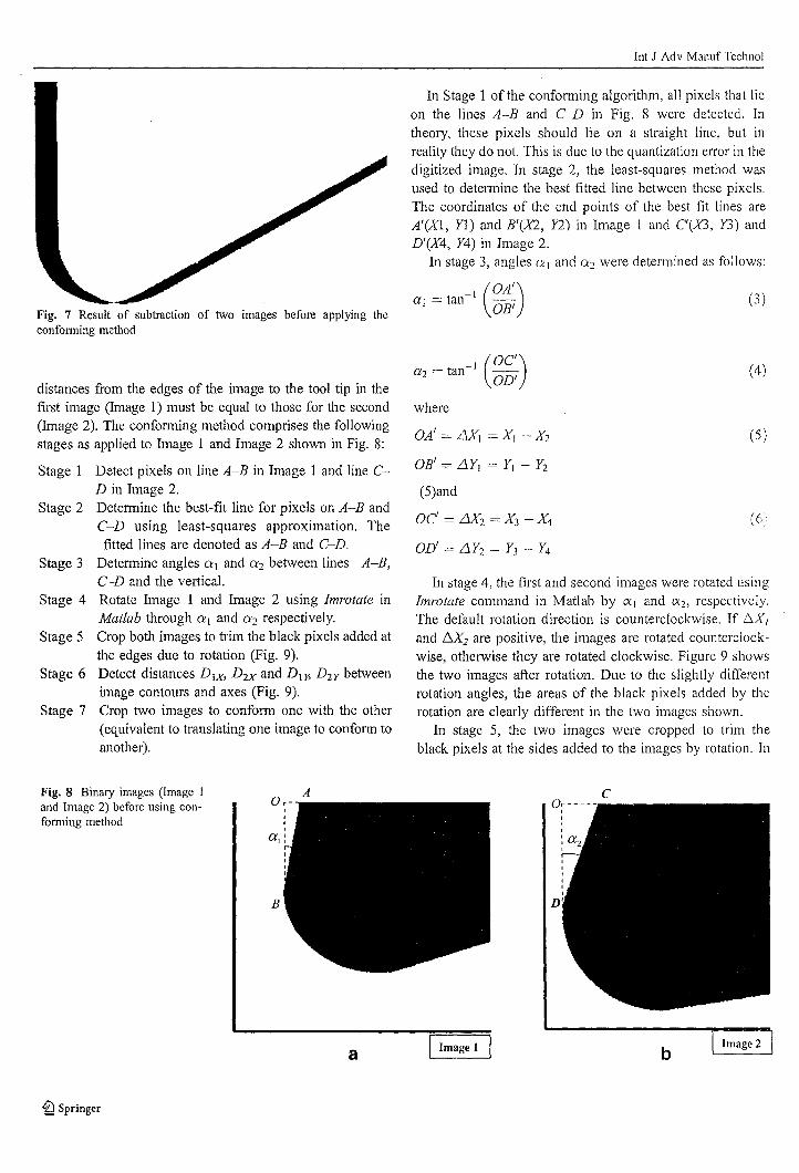
In Stage I of the confonning algorithm, all pixels that lieon the lines A-B and C-D in Fig. 8 were detected. Intheory, these pixels should lie on a straight line, but inreality they do not. This is due to the quantization error in thedigitized image. In stage 2, the least-squares method wasused to determine the best fitted line between these pixels.The coordinates of the end points of the best fit lines areA'(X!, Yl) and B'(X2, Y2) in Image 1 and C(X3, Y3) andD'(X4, Y4) in Image 2.

In stage 3, angles 01 and 02 were determined as follows:

In stage 4, the first and second images were rotated usingImrotate command in Matlab by {XJ and {X2, respectively.The default rotation direction is counterclockwise. If !:0{,

and /::0(2 are positive, the images are rotated counterclock­wise, otherwise they are rotated clockwise. Figure 9 showsthe two images after rotation. Due to the slightly differentrotation angles, the areas of the black pixels added by therotation are clearly different in the two images shown.

In stage 5, the two images were cropped to trim theblack pixels at the sides added to the images by rotation. In

Fig. 7 Result of subtraction of two images before applying theconforming method

distances from the edges of the image to the tool tip in thefirst image (Image 1) must be equal to those for the second(Image 2). The confonning method comprises the followingstages as applied to Image 1 and Image 2 shown in Fig. 8:

Stage 1 Detect pixels on line A-B in Image 1 and line c­D in Image 2.

Stage 2 Detennine the best-fit line for pixels on A-B andC-D using least-squares approximation. Thefitted lines are denoted as A-B and C-D.

Stage 3 Detennine angles 01 and 02 between lines A-B,C-D and the vertical.

Stage 4 Rotate Image I and Image 2 using Imrotate inMatlab through 01 and 02 respectively.

Stage 5 Crop both images to trim the black pixels added atthe edges due to rotation (Fig. 9).

Stage 6 Detect distances D 1X, D2X and D I !5 D2y betweenimage contours and axes (Fig. 9).

Stage 7 Crop two images to confOllli one with the other(equivalent to translating one image to confonn toanother).

(OA

I

)0'1 = tan-I OB'

(OC

I

)

OD'

where

OA' = LJXJ = XI - X2

OB' = LlY, = Y1 - Y2

(5)and

oC' = LJX2 = X3 - X4

OD' = LlY2 = Y3 - Y4

(3)

(4)

(5)

(6;

Fig. 8 Binary images (Image Iand Image 2) before using con­fomling method

a

~ Springer

I Image 1 I bI Image 2 I

Int J Adv Manuf Technol

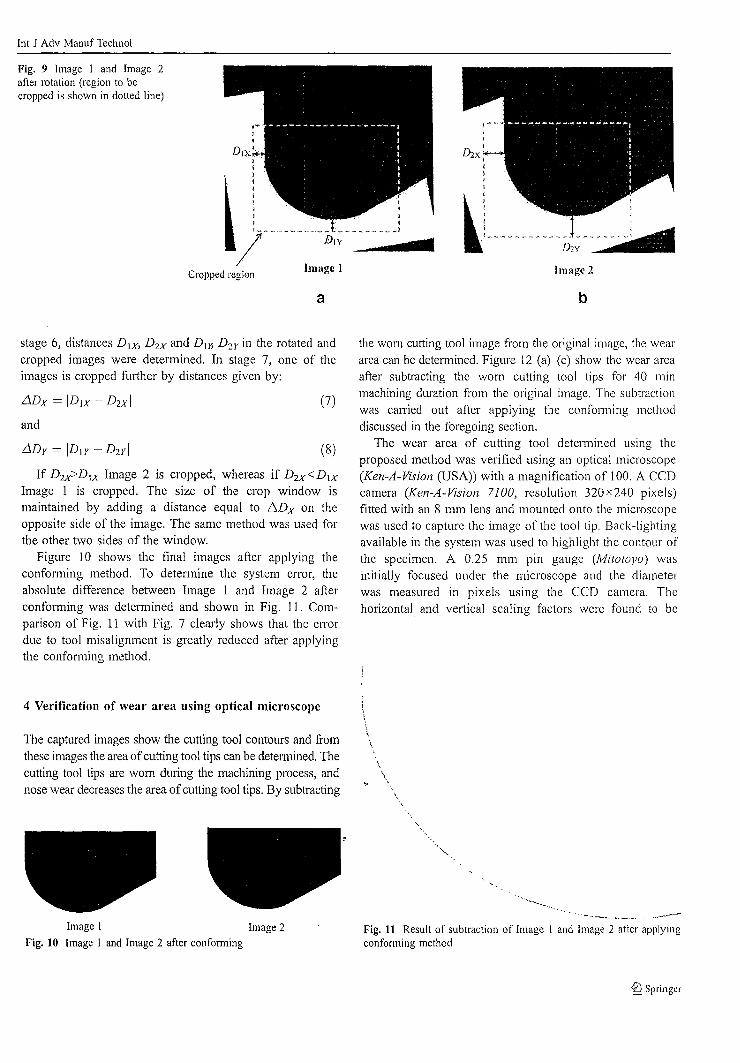
Fig. 9 Image I and Image 2after rotation (region to becropped is shown in dotted line)

;I""'.",,Drx',,

~ : m___ =I [m,::~ -_.....

Crpt'ped region

a

Image 2

b

stage 6, distances D 1X, D2X and D w Dzy in the rotated andcropped images were determined. In stage 7, one of theimages is cropped further by distances given by:

If D 2X>D tx Image 2 is cropped, whereas if D2X<D1X

Image 1 is cropped. The size of the crop window ismaintained by adding a distance equal to t::..Dx on theopposite side of the image. The same method was used forthe other two sides of the window.

Figure 10 shows the final images after applying theconfonning method. To determine the system error, theabsolute difference between Image 1 and Image 2 afterconfonning was determined and shown in Fig. 11. Com­parison of Fig. 11 with Fig. 7 clearly shows that the etTOrdue to tool misalignment is greatly reduced after applyingthe confonning method.

iJ.Dx = ID1.\:' - D2X Iand

(7)

(8)

the worn cutting tool image from the original image, the weararea can be detennined. Figure 12 (a)-(c) show the wear areaafter subtracting the worn cutting tool tips for 40 minmachining duration from the original image. The subtractionwas caJTied out after applying the confonning methoddiscussed in the foregoing section.

The wear area of cutting tool detetmined using theproposed method was verified using an optical microscope(Ken-A-Vision (USA)) with a magnification of 100. A CCDcamera (Ken-A-Vision 7100, resolution 320x240 pixels)fitted with an 8 mm lens and mounted onto the microscopewas used to capture the image of the tool tip. Back-lightingavailable in the system was used to highlight the contour ofthe specimen. A 0.25 mm pin gauge (Mitotoyo) wasinitially focused under the microscope and the diameterwas measured in pixels using the CCO camera. Thehorizontal and vertical scaling factors were found to be

4 Verification of wear area using optical microscope

The captured images show the cutting tool contours and fromthese images the area ofcutting tool tips can be detetmined. Thecutting tool tips are worn during the machining process, andnose wear decreases the area ofcutting tool tips. By subtracting

\."

- _--

Image I Image 2

Fig. 10 Image I and Image 2 after confoffi1ingFig. 11 Result of subtraction of Image 1 and Image 2 after applyingconforming method

~ Springer

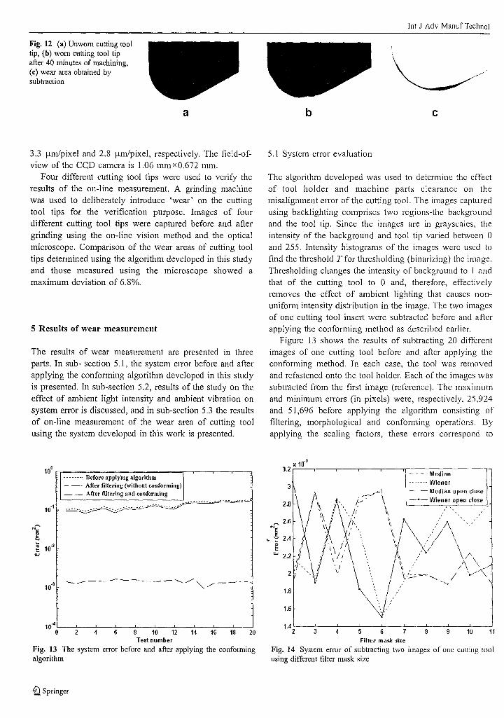
Fig. 12 (a) Unwom cutting tooltip, (b) wom cutting tool tipafter 40 minutes of machining,(c) wear area obtained bysubtraction

lnt J Adv Manuf Technol

a b c

3.3 11m/pixel and 2.8 11m/pixel, respectively. The field-of­view of the CCD camera is 1.06 mm x 0.672 mm.

Four different cutting tool tips were used to verify theresults of the on-line measurement. A grinding machinewas used to deliberately introduce 'wear' on the cuttingtool tips for the verification purpose. Images of fourdifferent cutting tool tips were captured before and aftergrinding using the on-line vision method and the opticalmicroscope. Comparison of the wear areas of cutting tooltips determined using the algorithm developed in this studyand those measured using the microscope showed amaximum deviation of 6.8%.

5 Results of wear measurement

The results of wear measurement are presented in threeparts. In sub- section 5.1, the system elTor before and afterapplying the confonning algorithm developed in this studyis presented. In sub-section 5.2, results of the study on theeffect of ambient light intensity and ambient vibration onsystem elTor is discussed, and in sub-section 5.3 the resultsof on-line measurement of the wear area of cutting toolusing the system developed in this work is presented.

10° n==============;,-..--..----,,...--,........ Before applying algorithm-- After filtering (withont conforming)- - Arter filtering and conforming

10·4 '--_'-_'--_'-_'--_'--_'--_'--_'------JL----..Jo 2 4 6 8 10 12 14 16 18 20

Test number

Fig. 13 The system error before and after applying the conformingalgorithm

%l Springer

5.1 System elTor evaluation

The algorithm developed was used to determine the effectof tool holder and machine parts clearance on themisalignment error of the cutting tool. The images capturedusing backlighting comprises two regions-the backgroundand the tool tip. Since the images are in grayscales, theintensity of the background and tool tip varied between 0and 255. Intensity histograms of the images were used tofind the threshold T for thresholding (binarizing) the image.Thresholding changes the intensity of background to I andthat of the cutting tool to 0 and, therefore, effectivelyremoves the effect of ambient lighting that causes non­unifonn intensity distlibution in the image. The two imagesof one cutting tool insert were subtracted before and afterapplying the conforming method as described earlier.

Figure 13 shows the results of subtracting 20 di ffcrcntimages of one cutting tool before and after applying theconfonning method. In each case, the tool was removedand refastened onto the tool holder. Each of the images wassubtracted from the first image (reference). The maximumand minimum elTors (in pixels) were, respectively, 25,924and 51,696 before applying the algorithm consisting offiltering, morphological and conforming operations. Byapplying the scaling factors, these enol'S correspond to

1.42'---'-3--4'----'-5--6'---'-7--'----'-----'10-----'11

Filter mask size

Fig. 14 System error of subtracting two images of one cutting toolusing different filter mask size

Int J Adv Manuf Techno!

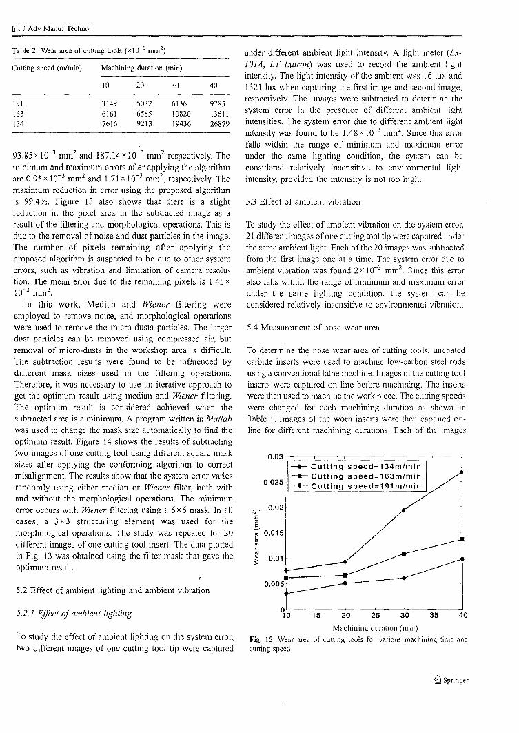
Table 2 Wear area of cutting tools (x 10-6 mm2)

5.2 Effect of ambient lighting and ambient vibration

93.85xlO-3 mm2 and 187.14xlO-3 mm2 respectively. The

minimum and maximum errors after applying the algorithmare 0.95X 10-3 mm2 and 1.71 x 10-3 mm2

, respectively. Themaximum reduction in error using the proposed algorithmis 99.4%. Figure 13 also shows that there is a slightreduction in the pixel area in the subtracted image as aresult of the filtering and morphological operations. This isdue to the removal of noise and dust particles in the image.The number of pixels remaining after applying theproposed algorithm is suspected to be due to other systemelTors, such as vibration and limitation of camera resolu­tion. The mean error due to the remaining pixels is 1.45 x

10-3 mm2.

In this work, Median and Wiener filtering wereemployed to remove noise, and morphological operationswere used to remove the micro-dusts particles. The largerdust particles can be removed using compressed air, butremoval of micro-dusts in the workshop area is difficult.The subtraction results were found to be influenced bydifferent mask sizes used in the filtering operations.Therefore, it was necessary to use an iterative approach toget the optimum result using median and Wiener filtering.The optimum result is considered achieved when thesubtracted area is a minimum. A program wtitten in Matlabwas used to change the mask size automatically to find theoptimum result. Figure 14 shows the results of subtractingtwo images of one cutting tool using different square masksizes after applying the confonning algorithm to correctmisalignment. The results show that the system error variesrandomly using either median or Wiener filter, both withand without the morphological operations. The minimumerror occurs with Wiener filtering using a 6 x 6 mask. In allcases, a 3 x 3 structuring element was used for themorphological operations. The study was repeated for 20different images of one cutting tool insert. The data plottedin Fig. 13 was obtained using the filter mask that gave theoptimum result.

0.Q1

0.03 r;=--+-==cC::::u=tt=i=n=g::=s=p=e=e=d::':==1=3=4=m=:O::/=m=i=n=;-~---1

--- Cutting speed=163m/min-+- Cutting speed=191 m/min0.025

'" 0.015~....'"'l)~

0.005

~ 0.02('6S

under different ambient light intensity. A light meter (Lx­lOlA, LT Lutron) was used to record the ambient lightintensity. The light intensity of the ambient was 16 lux and1321 lux when capturing the first image and second image,respectively. The images were subtracted to determine thesystem error in the presence of different ambient lightintensities. The system error due to different ambient lightintensity was found to be 1.48 x 10-3 mm2

. Since this errorfalls within the range of minimum and maximum errorunder the same lighting condition, the system can beconsidered relatively insensitive to environmental lightintensity, provided the intensity is not too high.

To study the effect of ambient vibration on the system error,21 different images ofone cutting tool tip were captured underthe same ambient light. Each of the 20 images was subtractedfrom the first image one at a time. The system error due toambient vibration was found 2x 10-3 mm". Since this erroralso falls within the range of minimum and maximum errorunder the same lighting condition, the system can beconsidered relatively insensitive to environmental vibration.

5.3 Effect of ambient vibration

To determine the nose wear area of cutting tools, uncoatedcarbide inserts were used to machine low-carbon steel rodsusing a conventional lathe machine. Images of the cutting toolinselts were captured on-line before machining. The inseltswere then used to machine the work piece. The cutting speedswere changed for each machining duration as shown inTable 1. Images of the worn inselts were then captured on­line for different machining durations. Each of the images

5.4 Measurement of nose wear area

97851361126879

4030

61361082019436

503265859213

2010

Machining duration (min)

314961617616

191163134

Cutting speed (m/min)

5.2.1 Effect ofambient lightingo'-__'---__"--__-'- -'--__-'--_---.-.J

10 15 20 25 30 35 40

To study the effect of ambient lighting on the system error,two different images of one cutting tool tip were captured

Machining duration (min)

Fig. 15 Wear area of cutting tools for various machining time andcutting speed

~ Springer

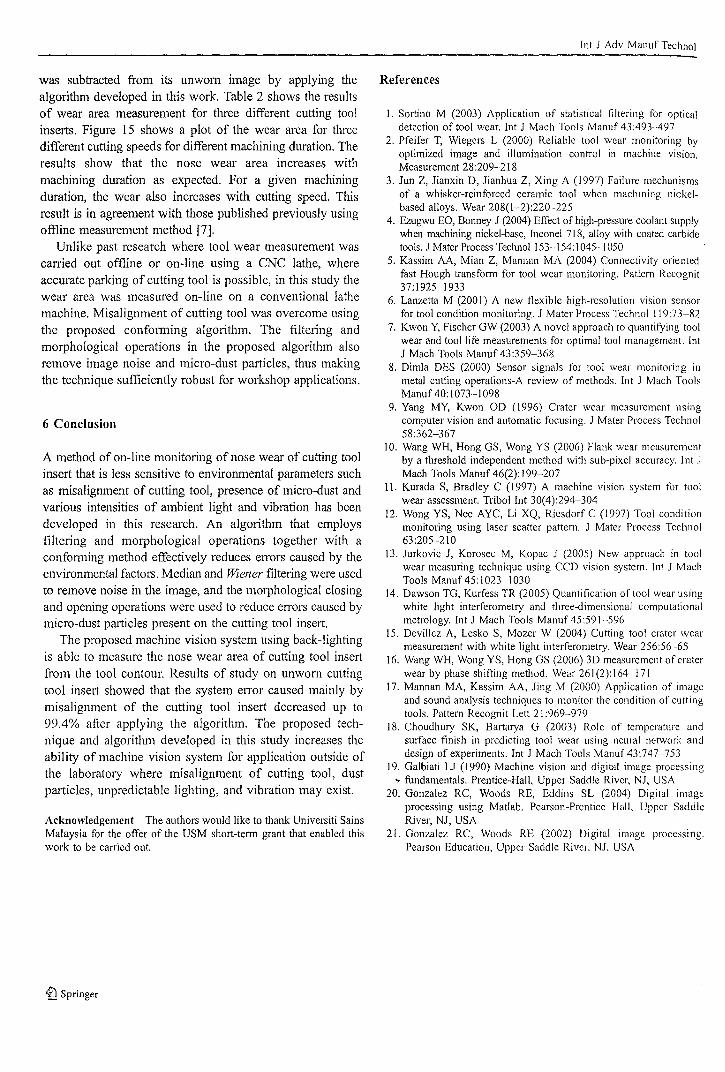
was subtracted from its unwom image by applying thealgorithm developed in this work. Table 2 shows the resultsof wear area measurement for three different cutting toolinserts. Figure 15 shows a plot of the wear area for threedifferent cutting speeds for different machining duration. Theresults show that the nose wear area increases withmachining duration as expected. For a given machiningduration, the wear also increases with cutting speed. Thisresult is in agreement with those published previously usingoffline measurement method [7].

Unlike past research where tool wear measurement wascan'ied out offline or on-line using a CNC lathe, whereaccurate parking of cutting tool is possible, in this study thewear area was measured on-line on a conventional lathemachine. Misalignment of cutting tool was overcome usingthe proposed confOlming algorithm. The filtering andmorphological operations in the proposed algorithm alsoremove image noise and micro-dust particles, thus makingthe technique sufficiently robust for workshop applications.

6 Conclusion

A method of on-line monitoring of nose wear of cutting toolinsert that is less sensitive to environmental parameters suchas misalignment of cutting tool, presence of micro-dust andvarious intensities of ambient light and vibration has beendeveloped in this research. An algorithm that employsfiltering and morphological operations together with acontonning method effectively reduces errors caused by theenvironmental factors. Median and Wiener filtering were usedto remove noise in the image, and the morphological closingand opening operations were used to reduce errors caused bymicro-dust particles present on the cutting tool insert.

The proposed machine vision system using back-lightingis able to measure the nose wear area of cutting tool insertfrom the tool contour. Results of study on unworn cuttingtool insert showed that the system error caused mainly bymisalignment of the cutting tool insert decreased up to99.4% after applying the algorithm. The proposed tech­nique and algorithm developed in this study increases theability of machine vision system for application outside ofthe laboratory where misalignment of cutting tool, dustparticles, unpredictable lighting, and vibration may exist.

Acknowledgement The authors would like to thank Universiti SainsMalaysia for the offer of the USM short-term grant that enabled thiswork to be carried out.

~ Springer

[nt J Adv Manuf Technol

References

I. Sortino M (2003) Application of statistical filtering for opticaldetection of tool wear. [nt J Mach Tools Manuf 43 :493497

2. Pfeifer T, Wiegers L (2000) Reliable tool wear monitoring byoptimized image and illumination control in machine vision.Measurement 28:209-218

3. Jun Z, Jianxin D, Jianhua Z, Xing A (1997) Failure mechanismsof a whisker-reinforced ceramic tool when machining nickel­based alloys. Wear 208(1-2):220-225

4. Ezugwu EO, Bonney J (2004) Effect of high-pressure coolant supplywhen machining nickel-base, lnconel 718, alloy with coated carbidetools. J Mater Process Technol 153·154: I045·1050

5. Kassim AA, Mian Z, Mannan MA (2004) Connectivity orientedfast Hough transform for tool wear monitoring. Pattern Recognit37:1925-1933

6. Lanzetta M (2001) A new flcxible high-resolution vision sensorfor tool condition monitoring. J Mater Process Technol 119:73-82

7. Kwon Y, Fischer GW (2003) A novel approach to quantifying toolwear and tool life measurements for optimal tool management. IntJ Mach Tools Manuf 43:359-·368

8. Dimla DES (2000) Sensor signals for tool wear monitoring inmetal cutting operations-A review of methods. [nt J Mach ToolsManuf 40: [073-1098

9. Yang MY, Kwon OD (1996) Crater wear measurement usingcomputer vision and automatic focusing. J Mater Process Technol58:362-367

10. Wang WH, Hong GS, Wong YS (2006) Flank wear measurementby a threshold independent method with sub-pixel accuracy. Int .J

Mach Tools Manuf 46(2): 199-20711. Kurada S, Bradley C (1997) A machine vision system for tool

wear assessment. Tribol Int 30(4):294-30412. Wong YS, Nee AYC, Li XQ, Riesdorf C (1997) Tool condition

monitoring using laser scatter pattern. J Mater Process Technol63:205-210

13. Jurkovic J, Korosec M, Kopac J (2005) New approach in toolwear measuring technique using CCD vision system. Int J MachTools Manuf 45: 1023 .. 1030

14. Dawson TG, Kurfess TR (2005) Quantification of tool wear usingwhite light interferometry and three-dimensional computationalmetrology. Int J Mach Tools ManuI' 45:591596

15. Devillez A, Lesko S, Mozer W (2004) Cutting tool crater wearmeasurement with white light interferometry. Wear 256:56-65

16. Wang WH, Wong YS, Hong GS (2006) 3D measurement of craterwear by phase sh ifting method. Wear 261 (2): 164 171

17. Mannan MA, Kassim AA, Jing M (2000) Application of imageand sound analysis techniques to monitor the condition of cuttingtools. Pattern Recognit Lett 21 :969-979

18. Choudhury SK, Bartarya G (2003) Role of temperaturc andsurface finish in predicting tool wear using neural network anddesign of experiments. Int J Mach Tools Manuf 43:747-753

19. Galbiati LJ (1990) Machine vision and digital image processing.,. fundamentals. Prentice-Hall, Upper Saddle River, NJ, USA

20. Gonzalez RC, Woods RE, Eddins SL (2004) Digital imageprocessing using Matlab. Pearson-Prentice Hall, Upper SaddleRiver, NJ, USA

21. Gonzalez RC, Woods RE (2002) Digital image processing.Pearson Education, Upper Saddle River, NJ, USA

lnt J Adv Manuf Technol

DOII0.1007/s00170-008-1437-1

Notch wear detection in cutting tools using gradientapproach and polynomial fitting

H. H. Shahabi . T. H. Low· M. M. Ratnam

Received: 5 June 2007/Accepted: 8 February 2008(;) Springer-Verlag London Limited 2008

Abstract Cutting tool wear is well known to affect thesurface finish of a turned part. Various machine visionmethods have been developed in the past to measure andquantify tool wear. The two most widely measuredparameters in tool wear monitoring are flank wear andcrater wear. Works carried out by several researchersrecently have shown that notch wear has a more severeeffect on the surface roughness compared to flank or crater

wear. In this work, a novel gradient detection approach hasbeen developed to detect the presence of micro-scalenotches in the nose area of the cutting tool. This methodis capable of detecting the location of the notch accurately

from a single worn cutting tool image.

Keywords Notch wear· Cutting tool· Gradient detection·Polynomial fitting

1 Introduction

Vision-based systems are gammg considerable attentionfrom the research community for tool wear measurementdue to their numerous advantages, such as direct measure­ment of wear, non-contacting, high spatial resolution, high­speed data processing, visualization of wear area, etc.

Kurada et al. [1] gave a review of the basic principles,instrumentation and processing schemes used in various

machine vision sensors. Two of the most common types oftool wear measured are flank wear and crater wear [2].

H. H. Shahabi . T. H. Low' M. M. Ratnam ([gJ)School of Mechanical Engineering, Engineering Campus,University Sains Malaysia,14300 Nibong Tebal, Malaysiae-mail: mmaran@eng.usm.my

Flank wear occurs on the relief face of the cutting tool andis mainly caused by the rubbing action of the tool on themachined surface, while crater wear occurs on the rake faceof the tool. The criteria for tool life is based on the width ofthe flank wear land defined in the IS03685 standard [3].According to the standard, the maximum width of the flankwear land VB smax =O.6 mm if the flank wear is notregularly worn. If the flank wear land is regularly worn,

the criteria for tool life is the average width of the flankwear land VBs =O.3 mm.

Several researchers used machine vision methods tomeasure the flank wear directly in the past. For instance,Kurada et al. [2] used a series of image processingoperations that include image enhancement by linear andmedian filtering, segmentation using edge operators andfeature extraction to measure the maximum wear landwidth. Wang et al. [4] measured flank wear using a

threshold-independent edge-detection approach based onmoment invariance. In another publication, Wang et al. [5]measured flank wear by capturing and processing succes­sive images of a moving cutting tool. Pfeifer et al. [6]extracted the flank wear contour using optimized adjust­

ment of illumination, while Sortino [7] used a statisticalfiltering method to detect the worn edge of the cutting tool.{eon et al. [8] used real-time vision technology to monitorthe average and maximum peak values of the wear land.

Unlike flank wear, measurement of crater wear hasreceived less attention in the past. Wang et al. [9] appliedthe phase-shifting method using fringe projection to extract'the 3-D wear crater profile, while Jurkovic et al. [10]

measured both crater wear and flank wear using structured

lighting.Although flank wear has been extensively studied in the

past, Ghani et al. [11] have shown experimentally that for

some machining conditions the surface roughness of the

©Springer

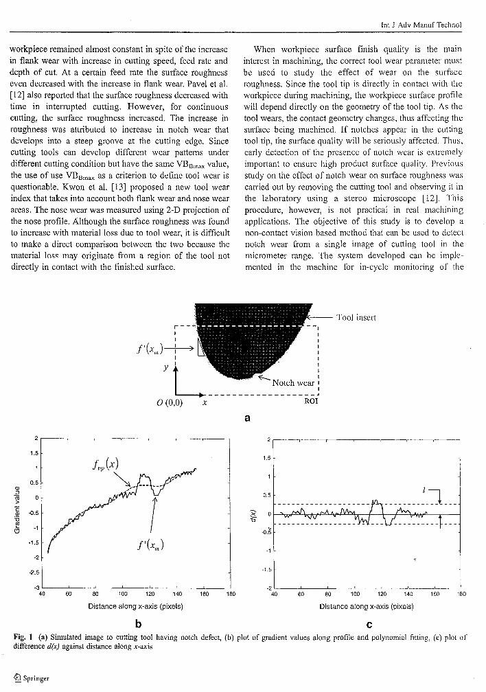
workpiece remained almost constant in spite of the increasein flank wear with increase in cutting speed, feed rate anddepth of cut. At a certain feed rate the surface roughnesseven decreased with the increase in flank wear. Pavel et al.[12] also reported that the surface roughness decreased withtime in interrupted cutting. However, for continuouscutting, the surface roughness increased. The increase inroughness was attributed to increase in notch wear thatdevelops into a steep groove at the cutting edge. Sincecutting tools can develop different wear patterns underdifferent cutting condition but have the same VBBmax value,the use of use VBBmax as a criterion to ddine tool wear isquestionable. Kwon et al. [13] proposed a new tool wearindex that takes into account both flank wear and nose wearareas. The nose wear was measured using 2-D projection ofthe nose profile. Although the surface roughness was foundto increase with material loss due to tool wear, it is difficultto make a direct comparison between the two because thematerial loss may originate from a region of the tool notdirectly in contact with the finished surface.

lnt J Adv Manuf Technol

When workpiece surface finish quality is the maininterest in machining, the correct tool wear parameter mustbe used to study the effect of wear on the surfaceroughness. Since the tool tip is directly in contact with theworkpiece during machining, the workpiece surface profilewill depend directly on the geometry of the tool tip. As thetool wears, the contact geometry changes, thus affecting thesurface being machined. If notches appear in the cuttingtool tip, the surface quality will be seriously affectcd. Thus,carly detection of the presence of notch wcar is extremelyimportant to ensure high product surfacc quality. Previousstudy on the effect of notch wear on surfacc roughncss wascarried out by removing the cutting tool and observing it inthe laboratory using a stereo microscope [12]. Thisprocedure, however, is not practical in real machiningapplications. The objective of this study is to develop anon-contact vision based method that can be used to dctcctnotch wear from a single image of cutting tool in themicrometer range. The system developed can be imple­mented in the machine for in-cycle monitoring of the

Tool insertr---ii

f'(x,J : )I I

YL ~_~~t~h_~~ac]0(0,0) x ROI

a

2

1.5

0.5(J)::>

Cii 0>C -0.5(J)

'5~ -1

<9

-1.5

-2

-2.5

-340 60 80 100

f'(x,J

120 140 160 180

-1

-1.5

-2 L....._---'-__-'-__-'--__

40 60 80 100 120 140 160 180

Distance along x-axis (pixels)

b

Distance along x-axis (pixels)

cFig. 1 (a) Simulated image to cutting tool having notch defect, (b) plot of gradient values along profile and polynomial fitting, (c) plot ofdifference d(x) against distance along x-axis

©Springer

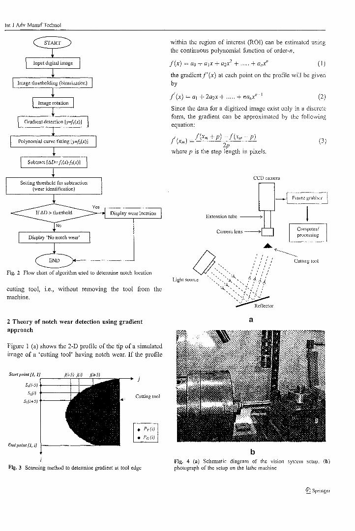
lnt J Adv Manuf Technol

(2)

( I )

!

(3)

Computer/processing

Frame grabber

() :' :'~~""i""OOI...... I I " I

" ", " I f I.. "', " , f I,'

, " ',~ "," ,Light source ",', , ~ , , " f...( ~

..... , ~ "', ',,' t / "~ ", I I

...... " '1 ... : ... :. /'~'{',.

"'... J' .. ,' "

" Reflector

Since the data for a digitized image exist only in a discretefonn, the gradient can be approximated by the followingequation:

the gradientf'(x) at each point on the profile will be givenby

within the region of interest (ROn can be estimated usingthe continuous polynomial function of order-n,

Extension tube -----:;>1

CCD camera

f'( ) _f(xm +p) -- f(x m -- p)

Xm -2p

where p is the step length in pixels.

f(x) = ao + ajX + a2x2 + ..... + aI/xII

Display wear location

Polynomial curve fitting [y=h(x)]

Image thresholding (binarization)

Setting threshold for subtraction(wear identification)

Fig. 2 Flow chart of algorithm used to detennine notch location

cutting tool, i.e., without removing the tool from themachine.

2 Theory of notch wear detection using gradientapproach

Figure 1 (a) shows the 2-D profile of the tip of a simulatedimage of a 'cutting tool' having notch wear. If the profile

a

b

j

• P y (i)

• Peri)

Cutting tool

Sdi-5) +-----+--+--::Sdi)

Sdi+5) t-----

Start poillt [1, 1]r-----,..---,c---,-----

Elld poillt [1, if

Fig. 3 Scanning method to detennine gradient at tool edgeFig. 4 (a) Schematic diagram of the vision system setup. (b)photograph of the setup on the lathe machine

~ Springer

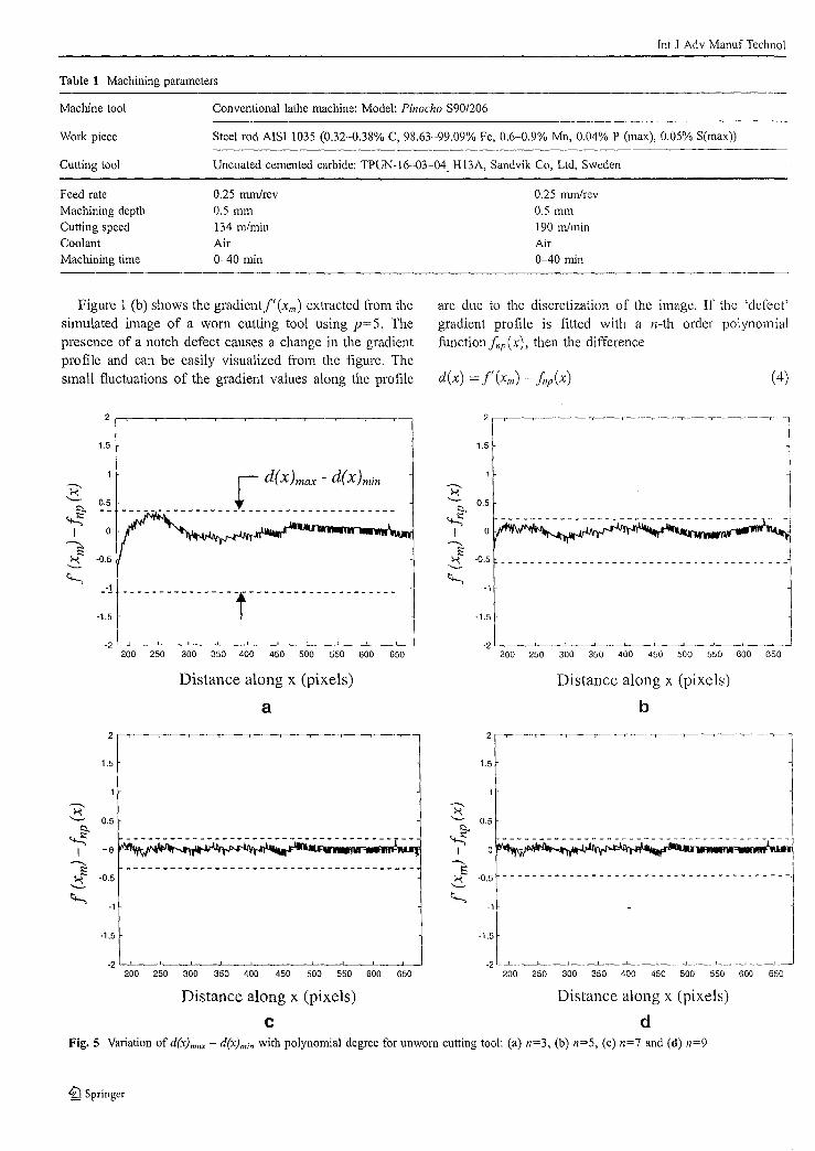
[nt J Adv Manuf Technol

Table 1 Machining parameters

Machine tool

Work piece

Cutting tool

Conventional lathe machine: Model: Pinocho S90/206

Steel rod AISI 1035 (0.32--0.38% C, 98.63-99.09% Fe, 0.6-0.9% Mn, 0.04% P (max), 0.05% S(max))

Uncoated cemented carbide: TPUN-16-03-04_HI3A, Sandvik Co, Ltd, Sweden

Feed rateMachining depthCutting speedCoolantMachining time

0.25 mrn/rev0.5 mm134 m/minAir0-40 min

0.25 mm/rev0.5 mm190 m/minAir0-40 min

are due to the discretization of the image. If the 'defect'gradient profile is fitted with a n-th order polynomialfunctionfnp(x), then the difference

Figure 1 (b) shows the gradient!, (xm) extracted from thesimulated image of a worn cutting tool using p=5. Thepresence of a notch defect causes a change in the gradientprofile and can be easily visualized from the figure. Thesmall fluctuations of the gradient values along the profile d(x) = f'(xm) - fnp(x) (4)

1.5

----.J -0.5

-:: ---------------~--------------------

2

1.5

---..~'-- 0.5

~<;...:;I 0

----;,.l::~ -0.5'--

~-1

-1.5

_C]

--------------------------------------1

-2 LJ._-"-_-'-_--'-_-'-_..L-_-'-_-'--_-'--_'---'200 250 300 350 400 450 500 550 600 650

Distance along x (pixels)

a

200 250 300 350 400 450 500 550 600 650

Distance along x (pixels)

b

1.5

0.5

~- -,:i.:n.: - - - - J~. - - - - - - - - - -,;.: - - - - - - - - - - - r - --9 - IW .". -,. '"""l'

----.J -0.5

-1

·1.5

-2 LJ._--'-_--'-_-'-_-'-_--'-_-'-_-'-_--'---_..L---I200 250 300 350 400 450 500 550 600 650

Distance along x (pixels)

C

2

1.5

---..~'-- 0.5

~<;...:;I 0

---..E::~ -0.5'--

~-1

-1.5

-2

l

1---------------------------------------

i--------------------------------------~

1J-....-_.L._--l

200 250 300 350 400 450 500 550 600 650

Distance along x (pixels)

dFig. 5 Variation of d('()mnx - d(X)min with polynomial degree for unworn cutting tool: (a) n=3, (b) n=5, (c) n=7 and (d) n=9

~ Springer

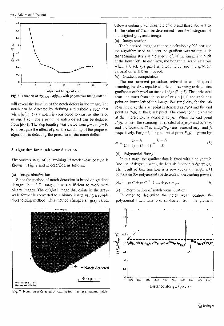
lnt J Adv Manuf Technol

0.2

1.6.,--------------------

3 Algorithm for notch wear detection

(6)

(5)

p(x) = P\Xn +p2'Y'-' + .... +PnX +PI7

(e) Determination of noteh wear locationIn order to determine the notch wear location, the

polynomial fitted data was subtracted from the gradient

below a certain pixel threshold T to 0 and those above T to1. The value of T can be determined from the histogram ofthe original grayscale image.(b) Image rotation

The binarized image is rotated clockwise by 90° becausethe algorithm used to detect the gradient was written suchthat scanning starts at the upper left of the image and endsat the lower left. In each row, the horizontal scanning stopswhen a black (0) pixel is encountered and the gradientcalculation will then proceed.(c) Gradient computation

The measurement procedure, refen-cd to as orthogonalscanning, involves repetitive horizontal scanning to detelminegradient at each pixel on the tool edge (Fig. 3). The horizontalscan line starts from the point of origin [1, I] and ends at apoint on lower left of the image. For simplicity, for the i-th

scan line Sdi) the stati point is denoted as Py(i) and the endpoint as Pdi) at the black pixel. The corresponding) valueat the intersection is denoted as j(i). When the end pointPeri) is met, the scanning is repeated at Sdi-p) and Sdi+p)and the locationsj(i-p) andj(i+p) are recorded as)\ andhrespectively. For p=5, the gradient at point Pc;(i) is given by:

h - j, h -)1m= =---

(i+5)-(i-5) 10

(d) Polynomial fIttingIn this stage, the gradient data is fitted with a polynomial

function of degree n using the Matlab function polyfit{-t,J',n).The result of this function is a row vector of length n+ 1containing the polynomial coefficients in descending powers:

30252015105O-l---~--~---~--~--~--__I

o

The various stage of determining of notch wear location isshown in Fig. 2 and is described as follows:

0.4

1.4

.::

~~ 0.8

><~ 0.6

1.2

(a) Image binarizationSince the method of notch detection is based on gradient

changes in a 2-D image, it was sufficient to work withbinary images. The original image that exists in the gray­scale format is converted to a binary image using a simplethresholding method. This method changes all gray values

will reveal the location of the notch defect in the image. Thenotch can be detected by defining a threshold t such thatwhen Id(x)1 > t a notch is considered to exist as illustratedin Fig. 1 (c). The size of the notch defect can be deducedfrom Id(x)l. The step lengthp was varied fromp=l to p=10to investigate the effect ofp on the capability ofthe proposedalgorithm in detecting the presence of the notch defect.

Polynomial fitting order, n

Fig. 6 Variation of d(x)max - d(>:)min with polynomial fitting order n

1.5

-... 0.5 /t~

c:..~~

I-...

~-1

-1.5

400 11mNotdlwearslaltsal520pixalNOlch wear ends 81554 pixel Distance along x (pixels)

Fig. 7 Notch wear detected on cutting tool having simulated notch

id Springer

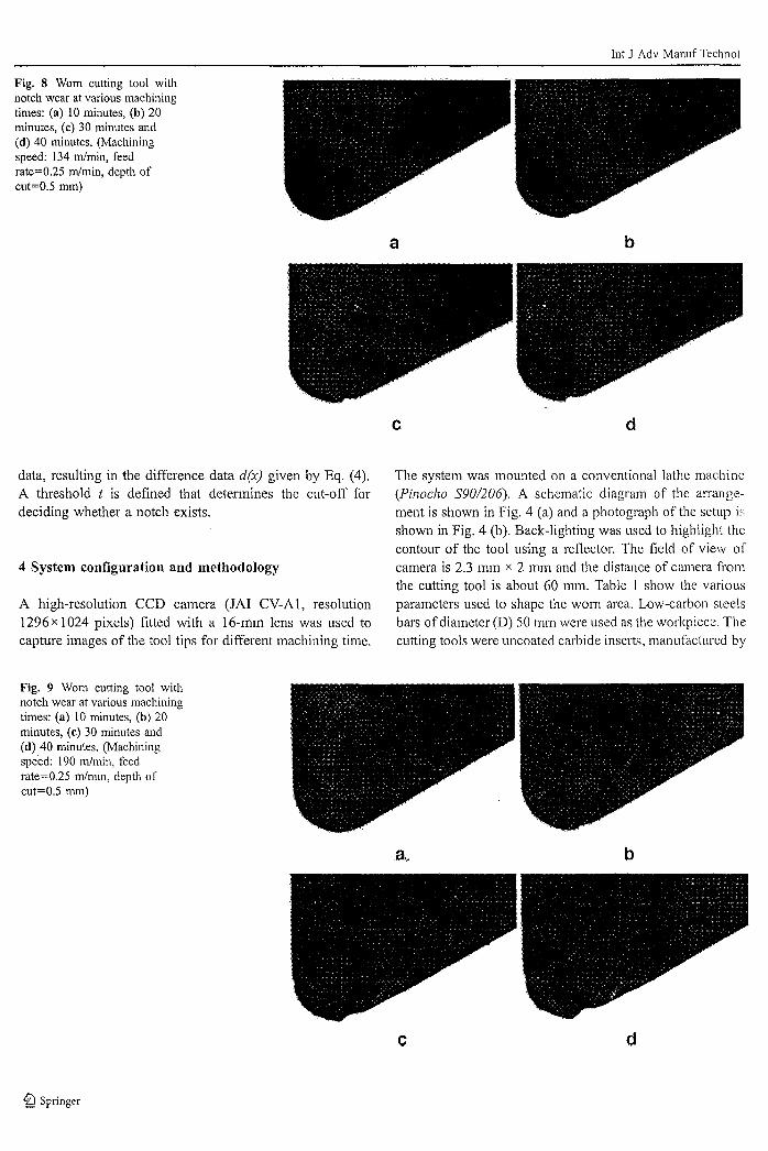
Fig. 8 Worn cutting tool withnotch wear at various machiningtimes: (a) 10 minutes, (b) 20minutes, (c) 30 minutes and(d) 40 minutes. (Machiningspeed: 134 m/min, feedrate=0.25 m/min, depth ofcut=0.5 mm)

Int J Adv Manuf Technol

a b

c d

data, resulting in the difference data d(x) given by Eq. (4).A threshold t is defined that determines the cut-off fordeciding whether a notch exists.

4 System configuration and methodology

A high-resolution CCD camera (JAI CV-Al, resolution1296x 1024 pixels) fitted with a 16-mm lens was used tocapture images of the tool tips for different machining time.

The system was mounted on a conventional lathe machine(Pinocho 590/206). A schematic diagram of the alTange­ment is shown in Fig. 4 (a) and a photograph of the setup isshown in Fig. 4 (b). Back-lighting was used to highlight thecontour of the tool using a reflector. The field of view ofcamera is 2.3 mm x 2 mm and the distance of camera fromthe cutting tool is about 60 mm. Table 1 show the variousparameters used to shape the worn area. Low-carbon steelsbars ofdiameter (D) 50 mm were used as the workpiece. Thecutting tools were uncoated carbide insel1s, manufactured by

Fig. 9 Worn cutting tool withnotch wear at various machiningtimes: (a) 10 minutes, (b) 20minutes, (c) 30 minutes and(d) 40 minutes. (Machiningspeed: 190 m/min, feedrate=0.25 m/min, depth ofcut=0.5 mm)

b

'f;) Springer

c d

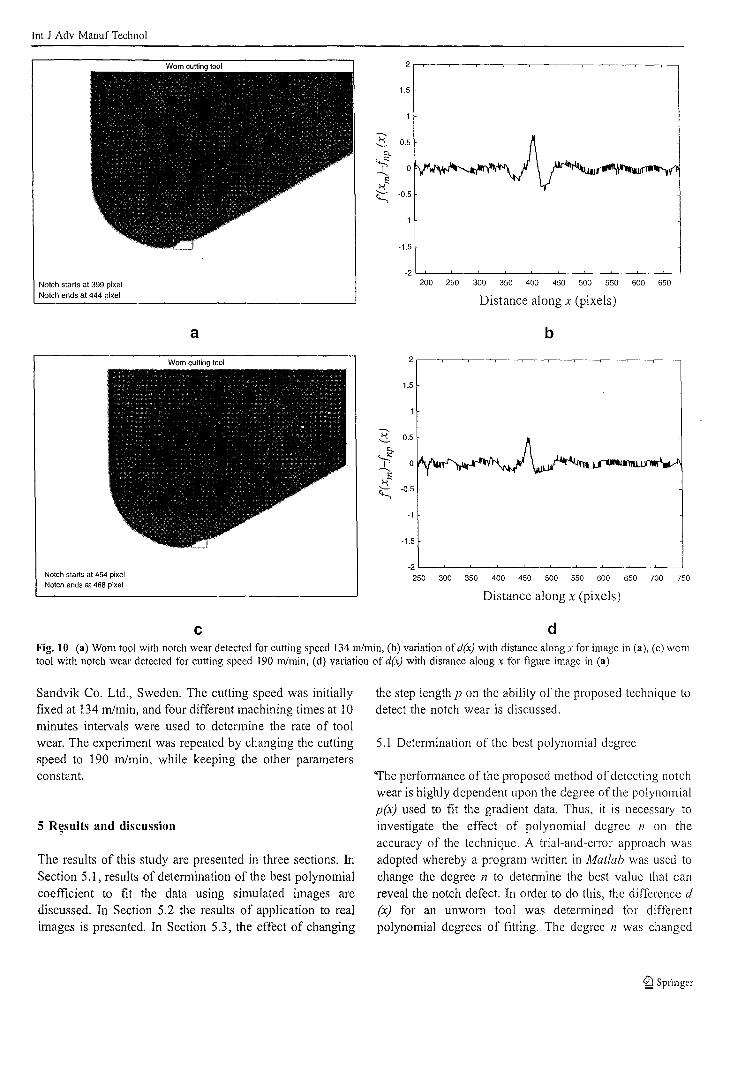
Int J Adv Manuf Technol

2

1.5

3 0.5

9-.....-;-

0I-...

~"t;::; -0.5

-1

-1.5

-2

Notch starts at 399 pixel 200 250 300 350 400 450 500 550 600 650

Notch ends at 444 pixel Distance along x (pixels)

a b

Worn cutting tool 2

1.5

-...~ 0.5

l:l..

~I-..."~"- -0.5

G-,

-1

-1.5

-2Notch starts at 454 pixel 250 300 350 400 450 500 550 600 650 700 750Notch ends at 488 pixel

Distance along x (pixels)

C dFig. 10 (a) Wom tool with notch wear detected for cutting speed 134 mlmin, (b) variation of d(.>:;) with distance along x for image in (a), (e) womtool with notch wear detected for cutting speed 190 mlmin, (d) variation of d(x) with distance along x for figure image in (a)

Sandvik Co. Ltd., Sweden. The cutting speed was initiallyfixed at 134 m/min, and four different machining times at 10minutes intervals were used to detet111ine the rate of toolwear. The experiment was repeated by changing the cuttingspeed to 190 m/min, while keeping the other parametersconstant.

5 R~sults and discussion

The results of this study are presented in three sections. InSection 5.1, results of detet111ination of the best polynomialcoefficient to fit the data using simulated images arediscussed. In Section 5.2 the results of application to realimages is presented. In Section 5.3, the effect of changing

the step length p on the ability of the proposed technique todetect the notch wear is discussed.

5.1 Determination of the best polynomial degree

"I'he performance of the proposed method of dctecting notchwear is highly dependent upon the degree of the polynomialp(x) used to fit the gradient data. Thus, it is necessary toinvestigate the effect of polynomial degree n on thcaccuracy of the techniquc. A trial-and-error approach wasadopted whereby a program wlitten in Matlah was used tochange the degree n to determine the best value that canreveal the notch defect. In order to do this, the difference d(x) for an unwom tool was detet111ined for differentpolynomial degrees of fitting. The degree n was changed

~ Springer

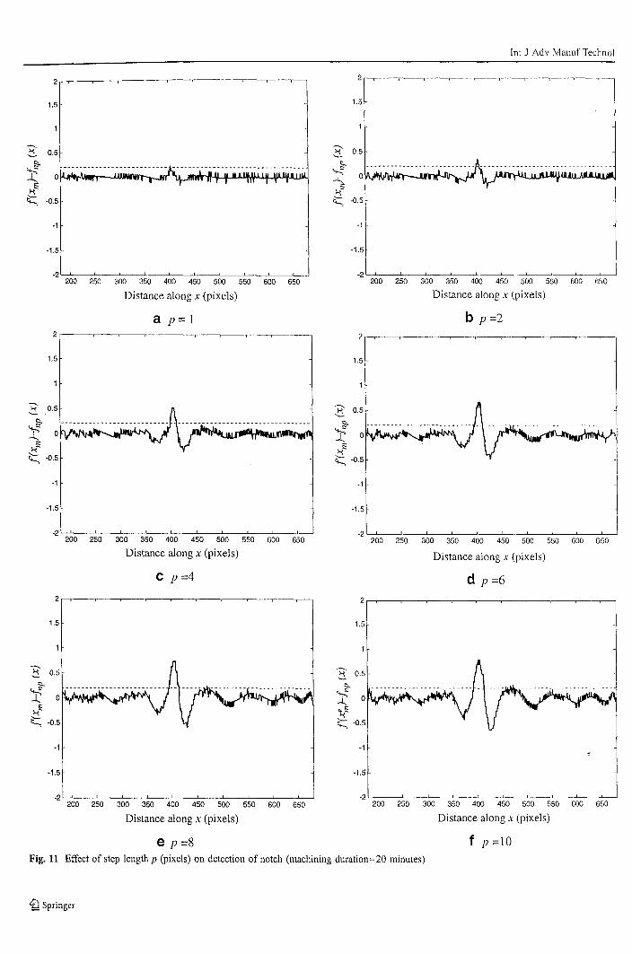
[nt J Adv Manuf Technol

1.5

--..~ 0.5

So...,.:;-l. 0

k,~

it:; -0.5

·1

-1.5

-2 '--'--'---'-------'-----'------'----'---'----'-------'--'200 250 300 350 400 450 500 550 600 650

Distance along x (pixels)

a p= 1

1.5

2 0.5

""~ 0I---;.,.k,'""- -0.5"'-.

-1

-1.5

-2 '--'---'-----'------'------'-------'---'-----'-----'-----'-----'~ ~ ~ ~ ~ ~ ~ ~ ~ B

Distance along x (pixels)

C p=4

1.5

-1

-1.5

-2 L2:-':0~0--:2::-50-=---,3:-':-0~0 --:3::-50.,---4::-00-=---4::-50.,---,5:-':-00.,---,5::-5~0 -6:-':-0-'0-6:-':-50----'

Distance along x (pixels)

2 ,..,--r---~-~-~.'---'-~---'~--'------'---_.----'...-

1.5

2 0.5

So...,.:;

0I---...;1

-0.5"'-.

-1

-1.5

-2 '--'__'-_-'----_...L--_---'--_--'-__'-_-'--_--'--_--'---!

~ ~ ~ ~ ~ ~ ~ ~ ~ ~

Distance along x (pixels)

b p=22,..,--r----.---~-....,..-~--r_-_.___-~-~___,

1.5

---..0.5k,

"-

""~I---..Ii:~"'-.

-1

-1.5

·2 '--'--'----'----'-----'-----'--'----'-------'-----'-------'200 250 300 350 400 450 500 550 600 650

Distance along x (pixels)

d p=6

1.5

---..~ 0.5

~'"'P~t;:::: -0.5

-1

-1.5

-2 '--'--'----'----'----'---------'---'-----'-----'---.:-':----'200 250 300 350 400 450 500 550 600 650

Distance along x (pixels)

e p=8Fig. 11 Effect of step length p (pixels) on detection of notch (machining duration=20 minutes)

~ Springer

f p =10

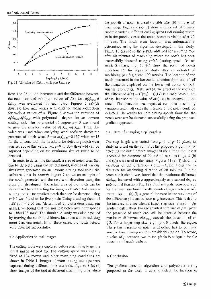
lnt J Adv Manuf Technol

5.2 Application to real images

the growth of notch is clearly visible after 20 minutes ofmachining. Figures 9 (a)-(d) show another set of imagescaptured under a different cutting speed (190 m/min) whereas in the previous case the notch becomes visible after 20minutes. The notch wear location was automaticallydetermined using the algorithm developed in this study.Figure 10 (a) shows the results obtained for a cutting toolafter 40 minutes of machining where the notch has beensuccessfully detected using t=0.2 (cutting speed 134 m/min). Similary, Fig. 10 (c) show the result of notchdetection for the repeated study after 20 minutes ofmachining (cutting speed 190 m/min). The location of thenotch measured in the horizontal direction from the left ofthe image is displayed on the lower left comer of bothimages. From Figs. 10 (b) and (d) the effect of the notch onthe difference d(x) = f'(xm) -.f~p(x) is clearly visible. Anabrupt increase in the value of d(x) can be observed at thenotch. The detection was repeated for other machiningdurations and in all cases the presence of the notch could bedetected. The results for both cutting speeds show that thenotch wear can be detected successfully using the proposedgradient approach.

The step length was varied from p= 1 to p= 10 pixels tostudy its effect on the ability of the proposed algorithm fordetecting the notch defect. Images of the cutting tool insel1machined for durations of 20 and 40 minutes (Figs. 8 (b)and (d) were used in this study. Figures 11 (a)-(f) show thevariation of the difference f'(xlIl ) -fl/p(x) along the x­direction for machining duration of 20 minutes. For thesame notch size it was found that the maximum differenced(x)l1lax increased with p approximately as a second degreepolynomial function (Fig. 12). Similar trends were observedfor the insert machined for 40 minutes (larger notch wear).From Figs. 11 (a)-(f) a general increase in the waviness ofthe difference plot can be seen as p increases. This is due tothe increase in error when a larger step size is used in thegradient calculation. For the smallest step size of p= I pixelthe presence of notch can still be detected because themaximum difference d(x)max exceeds the threshold of t=

g.2. For a larger step size, e.g., p> 10 pixels, the regionwhere the presence of notch is searched has to be madesmaller, thus missing notches outside this region. Therefore.a value of p between two to ten pixels is adequate for thedetection of notch defects.

5.3 Effect of changing step length p

10 II

Machining duration = 20 min

0. I +-........,---,---r--.,..--.,-----,---,---,--.,..--.,----j

°

from 3 to 25 in odd increments and the difference betweenthe maximum and minimum values of dr.,), i.e., d(x)ma[d(X)lIlif1 was evaluated for each case. Figures 5 (a)-(d)illustrate how d(x) varies with distance along x-directionfor various values of n. Figure 6 shows the variation ofd(x)max-d(X)mif1 with polynomial degree for an unworncutting tool. The polynomial of degree n= 15 was foundto give the smallest value of d(x)max-d(X)min' Thus, thisvalue was used when analyzing worn tools to detect thepresence of notch wear. Since d(x)max=0.137 when n=15for the unworn tool, the threshold for detecting notch wearwas set above this value, i.e., t=0.2. This threshold can beadjusted depending on the minimum size of notch to bedetected.

In order to determine the smallest size of notch wear thatcan be detected using the set threshold, notches of varioussizes were generated on an unworn cutting tool using thesoftware tools in Matlab. Figure 7 shows an example ofthe notch generated and the results of detection using thealgorithm developed. The actual area of the notch can bedetermined by subtracting the images of worn and unworncutting tools. The smallest notch that can be detected usingt=0.2 was found to be five pixels. Using a scaling factor of1.88 J.tm x 2.00 J.tm (determined by calibration using pingages), we found that the smallest notch area correspondsto 1.88 x 10-5 mm2

. The simulation study was also repeatedby moving the notch to different locations and introducingmore than one notch. In all these cases, the notch defectswere detected successfully.

1.3

I.l

0.9

j~ 0.7

0.5

0.3

Step length P (pixels)

Fig. 12 Variation of d(Y)max with step length p

The cutting tools were captured before machining to get theinitial image of tool tip. The cutting speed was initiallyfixed at 134 m/min and other machining conditions areshown in Table I. Images of worn cutting tool tips werecaptured during different time intervals. Figures 8 (a)-(d)show images of the tool at different machining time where

6 Conclusion

The gradient detection algorithm with polynomial fittingproposed in the work is able to detect the location of

©Springer

microscopic notch wear defects accurately from a single 2­D image of cutting tools. A camera mounted directly on thelathe machine enables image of the tool to be captured in­cycle (intermittently during machining) and analyzedwithout the need to dismantle the tool from the machine.Since previous researchers have shown that notch wear hasa direct effect on the surface roughness of the workpiece,the proposed technique can be use to detect problems earlyin the machining and prevent poor surface quality inproducts. The use of a single image overcomes the needfor positioning the camera accurately above the cutting tool.

Acknowledgement The authors would like to thank Universiti SainsMalaysia for the offer of the short-term grant that enabled this study tobe carried out and the reviewers for their valuable comments andcriticisms on this work.

References

1. Kurada S, Bradley C (1997) A review of machine vision sensorsfor tool condition monitoring. Computer in Industry 34:55-72

2. Kurada S, Bradley C (1997) A machine vision system for toolwear assessment. Tribol Int 30:295--304

%) Springer

Int 3 Adv Manuf Technol

3. International Standard (1993) Tool-life testing with single-pointturning tools: ISO 3685 2nd Edition, Switzerland

4. Wang WH, Hong GS, Wong YS (2006) Flank wear measurementby threshold independent method with sub-pixel accuracy. Int 3Mach Tools Manuf 46: 199-207

5. Wang WH, Wong YS, Hong GS (2005) Flank wear measurementby successive image analysis. Computer in Industry 56:816830

6. Pfeifer T, Wiegers L (2000) Reliable tool wear monitoring byoptimized image and illumination control in machine vision.Measurement 28:209--218

7. Sortino M (2003) Application of statistical filtering for opticaldetection of tool wear. Int J Mach Tools Manuf 43:493497

8. Jeon 3U, Kim SW (1988) Optical flank wear monitoring of cuttingtools by image processing. Wear 127:207-217

9. Wang WH, Wong YS, Hong GS (2006) 3D measurement of craterwear by phase shifting method. Wear 261:164-171

10. 3urkovic 3, Korosec M, Kopac J (2005) New approach in toolwear measuring technique using CCO vision system. Int J MachTools Manuf 45(2005): 1023-1 030

11. Ghani AK, Choudhury lA, Husni (2002) Study of tool life, surfaceroughness and vibration in machining nodular cast iron withceramic tool. 3 Mater Process Technol 127: 17-22

12. Pavel R, Marinescu 3, Deis M, Pillar J (2005) Effect of tool wearon surface finish for a case of continuous and intenupted hardturning. 3 Mater Process Technol 170(3):341-349

13. Kwon Y, Fischer GW (2003) A novel approach to quantifying toolwear and tool life measurements for optimal tool management. IntJ Mach Tools Manuf 43:359-368

at the

heldfrom

for the invention

18th- 20th May 2007

This is to certify that

has been awarded the

ITEX BRONZE MEDAL

TOOLMON: TOOL WEAR MONITORING ANDMEASUREMENT SYSTEM FOR LATHE MACHINES

18th International Invention, Innovation & Technology ExhibitionITEX 2007

Kuala Lumpur, Malaysia

ASSOC PROF DR MANI MARAN RATNAM, HAMIDREZAHSHAHABI

i,,I

it(~Y~~~~~l'!lWijXflf"~. ,

t • Q~ ~~J~l.... Invention - Innovation ~., Industrial Design - Technology

MINISTRY OF SCIENCE, MAL A Y 5 I A 0 ~TECHNOLOGY & INNOVATION ~~ MINDS ~

~tt,tt~~~~.~@~.~

~~~~~.,~tt,~~

~~

~~

~'l

~~," Dr Augustine 5'.' H. Ong ~.~,.~ President ~~ Malaysian Invention and Design Society ~

"~~~.A.~~~"'"'-~~ .

ttt ·