BOUNDARY LAYER STAGNATION POINT FLOW TOWARDSAN EXPONENTIALLY STRETCHING/SHRINKING SHEET

SAYED QASIM ALAVI

Thesis submitted in fulfilment of the requirementsfor the awards of the degree of

Master of Science (Mathematics)

Faculty of Industrial Sciences & TechnologyUNIVERSITI MALAYSIA PAHANG

October 2015

vi

ABSTRACT

The problem of boundary layer flow has many applications in industries andengineering field. Some of these applications are drawing of plastic films, glass fiberproduction, hot rolling and many others in industrial manufacturing processes. The finalproduct characteristics requested depends on the cooling liquid used and the rate ofstretching. Four common boundary conditions are used in modelling of convectiveboundary layer flow problems, which are constant or prescribed wall temperature,constant or prescribed surface heat flux, Newtonian heating and convective boundaryconditions. In this thesis, the mathematical modelling for the effects of radiation andMHD on stagnation point flow and heat transfer over an exponentiallystretching/shrinking sheet is investigated. In this study, the governing boundary layerequations are first transformed using an appropriate similarity transformation, which arethen solved numerically by using Keller-box method. MATLAB software is used as atool in order to obtain the numerical solution. Five parameters are investigated in thisproblem, which are Prandtl number Pr , velocity ratio parameter , conjugate parameter , magnetic parameter M and thermal radiation parameter RN . In conclusion, there

are dual solution when velocity ratio parameter satisfies 1.487068 0.9734 ,unique solution for 0.9734 and no solution exist for 1.487068 . To get aphysically acceptable value in second solution, the value of Prandtl number Pr must besmaller than a critical value Prc . It depends on conjugate parameter . While, the values

of conjugate parameter must be greater than some critical values c which also

depends on the Prandtl number Pr . Furthermore, increasing values of Prandtl numberPr and velocity ratio parameter has led to decrease in temperature profile while theincreasing in radiation parameter RN and magnetic parameter M has enhanced thetemperature profiles.

vii

ABSTRAK

Permasalahan aliran lapisan sempadan banyak diaplikasikan dalam industri dankejuruteraan. Aplikasi ini adalah pelakaran filem plastik, penghasilan gentian kaca,penggelekan panas dan pelbagai proses dalam industri pembuatan. Ciri-ciri produkakhir bergantung kepada cecair pendingin yang digunakan dan kadar perengangan.Kebiasaannya, terdapat empat syarat sempadan digunakan untuk pemodelan olakanaliran lapisan sempadan, antaranya adalah suhu dinding malar atau tetap, fluks habamalar atau tetap, pemanasan Newtonian dan syarat sempadan olakan. Dalam tesis ini,pemodelan matematik bagi kesan-kesan sinaran termal dan MHD ke atas aliran titikgenangan pemindahan haba melepasi lapisan meregang/mengecut secara eksponendikaji. Dalam kajian ini, persamaan menakluk lapisan sempadan pertama sekalidijelmakan dengan menggunakan kaedah penjelmaan setara yang sesuai, kemudiannyadiselesaikan secara berangka dengan menggunakan kaedah kotak Keller. PerisianMATLAB digunakan sebagai program komputer untuk pengekodan berangka. Limaparameter digunakan dalam permasalahan ini, iaitu nombor Prandtl Pr, parameter nisbahhalaju , parameter konjugat , parameter magnetik M dan parameter sinaran terma

RN . Kesimpulannya, permasalahan ini mempunyai dwi penyelesaian iaitu apabila

parameter nisbah halaju memenuhi ketaksamaan 1.487068 0.9734, penyelesaian unik bagi 0.9734 dan ketidakwujudan penyelesaian persamaan bagi

1.487068 . Bagi memperoleh nilai fizikal yang boleh diterima untuk penyelesaiankedua, nilai Pr mestilah lebih kecil daripada nilai kritikal Prc dan ia bergantung kepada

nilai , manakala nilai parameter konjugat mestilah lebih besar daripada nilai

kritikal c , yang juga bergantung kepada nilai Pr. Tambahan lagi, peningkatan nombor

Prandtl Pr dan parameter nisbah halaju memberi kesan kepada penyusutan suhuprofil manakala peningkatan parameter sinaran terma RN and parameter magnetik M

meningkatkan suhu profil.

viii

TABLE OF CONTENTS

Page

SUPERVISOR’S DECLARATION ii

STUDENT’S DECLARATION iii

DEDICATION iv

ACKNOWLEDGEMENT v

ABSTRACT vi

ABSTRAK vii

TABLE OF CONTENTS viii

LIST OF TABLES xi

LIST OF FIGURES xiii

LIST OF SYMBOLS xvii

LIST OF ABBREVIATIONS xix

CHAPTER 1 PRELIMINERIES

1.1 Introduction 1

1.2 Boundary Layer Theory 2

1.3 Boundary Conditions 3

1.3.1 Constant/Prescribed Wall Temperature 31.3.2 Constant/Prescribed Surface Heat Flux 41.3.3 Convective Boundary Conditions 5

1.4 Keller-Box Method 6

1.5 Stagnation Point 7

1.6 Research Objective 8

1.7 Research Scope 8

1.8 Literature Review 8

1.8.1 Boundary Layer Stagnation Point Flow over aStretching/Shrinking Sheet

8

1.8.2 Boundary Layer Stagnation Point Flow over anExponentially Stretching/Shrinking Sheet

12

1.8.3 Radiation Effects on MHD of the Boundary Layer StagnationPoint Flow over an Exponentially Stretching/Shrinking Sheet

14

ix

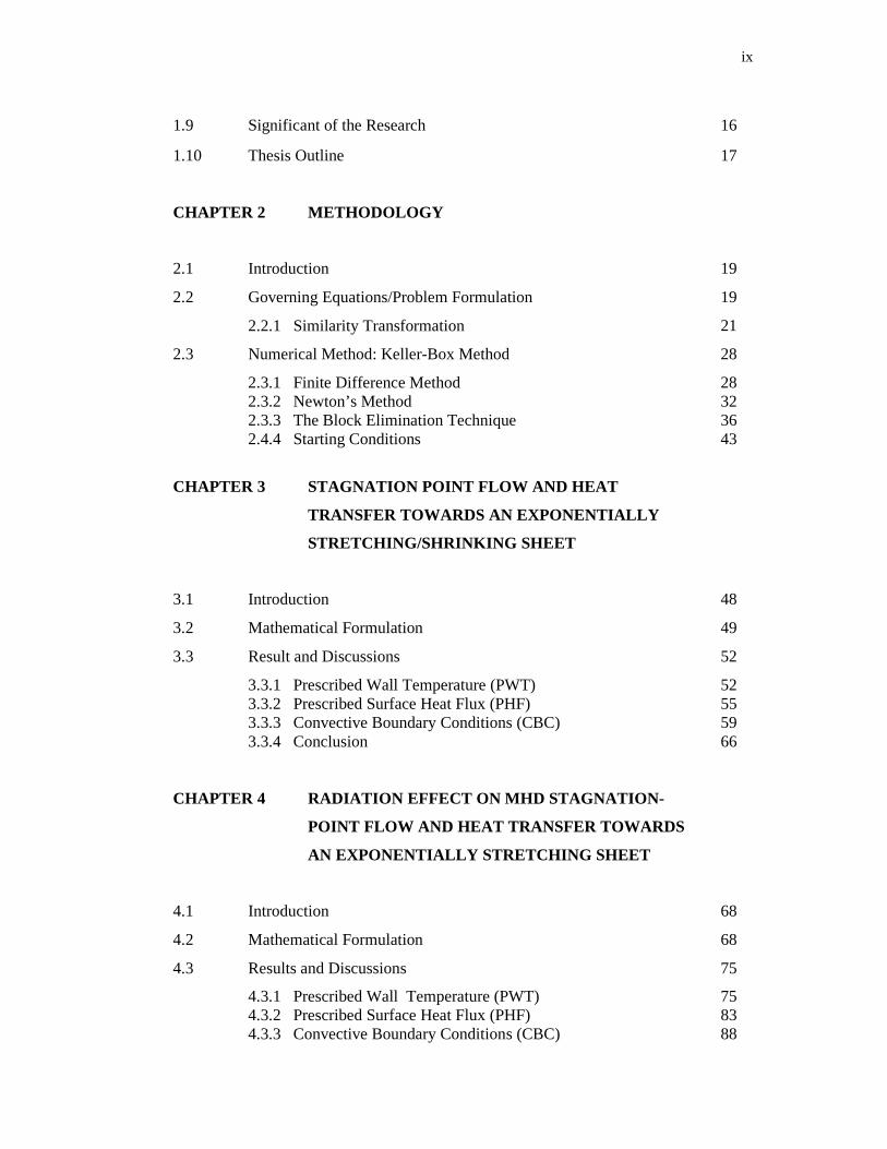
1.9 Significant of the Research 16

1.10 Thesis Outline 17

CHAPTER 2 METHODOLOGY

2.1 Introduction 19

2.2 Governing Equations/Problem Formulation 19

2.2.1 Similarity Transformation 21

2.3 Numerical Method: Keller-Box Method 28

2.3.1 Finite Difference Method 282.3.2 Newton’s Method 322.3.3 The Block Elimination Technique 362.4.4 Starting Conditions 43

CHAPTER 3 STAGNATION POINT FLOW AND HEAT

TRANSFER TOWARDS AN EXPONENTIALLY

STRETCHING/SHRINKING SHEET

3.1 Introduction 48

3.2 Mathematical Formulation 49

3.3 Result and Discussions 52

3.3.1 Prescribed Wall Temperature (PWT) 523.3.2 Prescribed Surface Heat Flux (PHF) 553.3.3 Convective Boundary Conditions (CBC) 593.3.4 Conclusion 66

CHAPTER 4 RADIATION EFFECT ON MHD STAGNATION-

POINT FLOW AND HEAT TRANSFER TOWARDS

AN EXPONENTIALLY STRETCHING SHEET

4.1 Introduction 68

4.2 Mathematical Formulation 68

4.3 Results and Discussions 75

4.3.1 Prescribed Wall Temperature (PWT) 754.3.2 Prescribed Surface Heat Flux (PHF) 834.3.3 Convective Boundary Conditions (CBC) 88

x

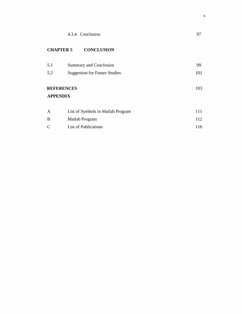
4.3.4 Conclusion 97

CHAPTER 5 CONCLUSION

5.1 Summary and Conclusion 99

5.2 Suggestion for Future Studies 101

REFERENCES 103

APPENDIX

A List of Symbols in Matlab Program 111

B Matlab Program 112

C List of Publications 116

xi

LIST OF TABLES

Table No Title Page

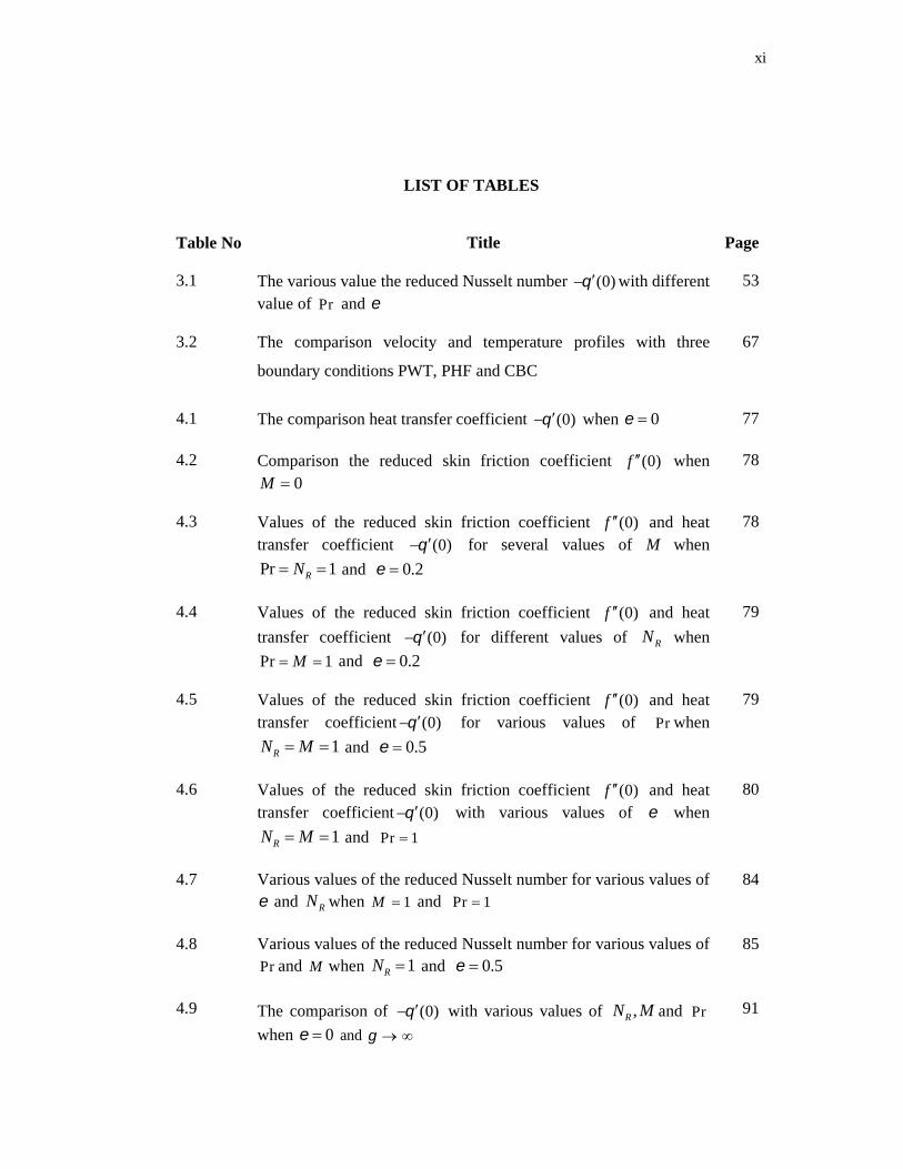
3.1 The various value the reduced Nusselt number (0) with differentvalue of Pr and

53

3.2 The comparison velocity and temperature profiles with three

boundary conditions PWT, PHF and CBC

67

4.1 The comparison heat transfer coefficient (0) when 0 77

4.2 Comparison the reduced skin friction coefficient (0)f when0M

78

4.3 Values of the reduced skin friction coefficient (0)f and heattransfer coefficient (0) for several values of M when

Pr 1RN and 0.2

78

4.4 Values of the reduced skin friction coefficient (0)f and heat

transfer coefficient (0) for different values of RN when

Pr 1M and 0.2

79

4.5 Values of the reduced skin friction coefficient (0)f and heattransfer coefficient (0) for various values of Pr when

1RN M and 0.5

79

4.6 Values of the reduced skin friction coefficient (0)f and heattransfer coefficient (0) with various values of when

1RN M and Pr 1

80

4.7 Various values of the reduced Nusselt number for various values of and RN when 1M and Pr 1

84

4.8 Various values of the reduced Nusselt number for various values ofPr and M when 1RN and 0.5

85

4.9 The comparison of (0) with various values of ,RN M and Pr

when 0 and

91

xii

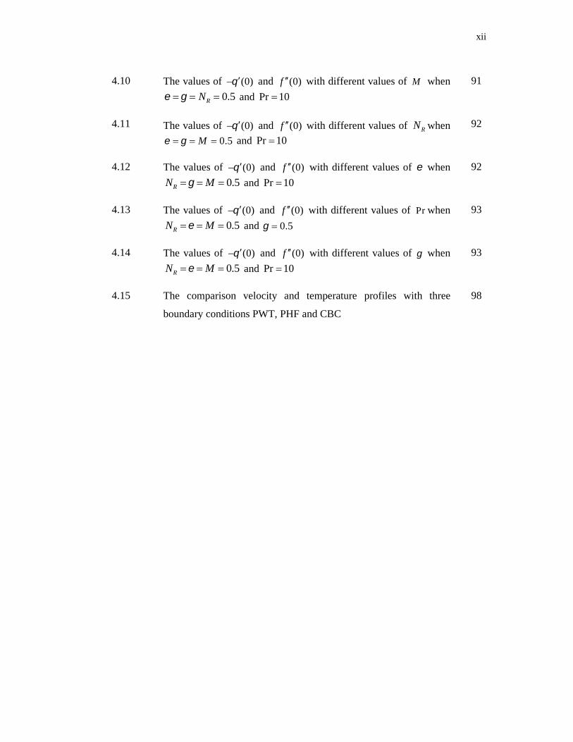
4.10 The values of (0) and (0)f with different values of M when

0.5RN and Pr 1091

4.11 The values of (0) and (0)f with different values of RN when

0.5M and Pr 10

92

4.12 The values of (0) and (0)f with different values of when

0.5RN M and Pr 1092

4.13 The values of (0) and (0)f with different values of Pr when

0.5RN M and 0.5

93

4.14 The values of (0) and (0)f with different values of when

0.5RN M and Pr 1093

4.15 The comparison velocity and temperature profiles with three

boundary conditions PWT, PHF and CBC

98

xiii

LIST OF FIGURES

Figure No Title Page

1.1 Velocity and thermal boundary layer 2

2.1 Physical model and coordinate system 20

2.2 Net rectangle for difference approximations 29

2.3 Flow diagram for the Keller-box method 46

3.1 Comparison of the reduced skin friction coefficient (0)f withdifferent values of

53

3.2 Comparison of the reduced Nusselt number (0) with differentvalues of when Pr 0.2

54

3.3 Variation of temperature profile ( ) with different values ofPr 0.2,1,3,7,10 when 0.5

54

3.4 Variation of temperature profile ( ) with different values of0.7,0.7,3,7,10 when Pr 0.2

55

3.5 The value of1

2Rex xNu with 56

3.6 Variation of velocity profiles ( )f with various values of whenPr 0.2

57

3.7 Variation of temperature profiles ( ) with different values of3,5,7,9 when Pr 0.7

57

3.8 Variation of temperature profile ( ) with different values ofPr 0.3,0.5,0.7,1,3 when 3

58

3.9 Variation of velocity profile f with different values of

3,5,7,10 when Pr 0.7

58

3.10 Variation of velocity profile f with different values of

0.7, 0.3,0.3,0.7 when Pr 0.7

59

xiv

3.11 Variation of the reduced skin friction coefficient (0)f with whenPr 0.2 and 0.5

61

3.12 Comparison of the reduced Nusselt number (0) with differentvalues of when Pr 0.2 and

61

3.13 Variation of the temperature (0) with when Pr 0.2 and0.5

62

3.14 Variation of the temperature (0) with Pr when 0.5,1 and1.2

62

3.15 Variation of the temperature (0) with when Pr 0.2 and1.2

63

3.16 Temperature profile ( ) for various values of 1.1, 1.2, 1.3 when Pr 0.2 and 0.5

63

3.17 Temperature profile for various values of Pr 0.1,0.2,0.25when 1.2 and 0.5

64

3.18 Temperature profile ( ) for various values of 0.5, 1,2 whenPr 0.2 and 1.2

64

3.19 Velocity profiles f for different values of 1.1, 1.2, 1.3 when Pr 0.2 and 0.5

65

3.20 Velocity profiles ( )f for different values of0.2,0.3,0.7,1.0,1.3,1.7,2.2 when Pr 0.2 and 0.5

65

4.1 Physical model and coordinate system 69

4.2 The velocity profile ( )f with for different values of

0,0.5,1,1.5,2 when Pr 1RN and 0.1M 80

4.3 The velocity profile ( )f with for different values of

0,0.5,1M when 0.1, 2 and Pr 1RN 81

4.4 The temperature profile ( ) with for different values of

0.1, 0.5, 1, 2, 4 when Pr 1RN and 1M

81

4.5 The temperature profile ( ) with for different values of

Pr 0.5, 1, 2, 4, 7 when 1RN and 1M

82

xv

4.6 The temperature profile ( ) with for different values of

0.5, 1, 2, 4RN when Pr 1 and 1M

82

4.7 The temperature profile ( ) with for different values of

0, 1, 2, 4M when Pr 1RN and 0.2 83

4.8 The temperature profile ( ) with for different values of

0.1, 0.5, 1, 2 when Pr 1RN and 1M

85

4.9 The temperature profile ( ) with for different values of

Pr 0.5, 1, 2, 4, 7 when 1RN and 1M

86

4.10 The temperature profile ( ) with for different values of

0, 1, 2, 4M when Pr 1RN and 0.2 86

4.11 The temperature profile ( ) with for different values of

0.5, 1, 2, 4RN when Pr 1 and 1M

87

4.12 The velocity profile ( )f with for different values of

0.3,0.5,0.7, 1.3, 1.5, 1.7 when Pr 1RN and 0.5M 87

4.13 The velocity profile ( )f with for different values of

0.0,0.3,0.5,0.7, 0.9M when 0.2,2 and Pr 1RN 88

4.14 The temperature profiles ( ) for several values of

0,2, 0.5, 1,2M when Pr 0.5RN and 0.5

94

4.15 The temperature profiles ( ) for several values of

0.2, 0.5, 1,2RN when Pr 0.5M and 0.5

94

4.16 The temperature profiles ( ) for several values of

0,2, 0.5, 1,2 when Pr 0.5M and 0.5RN 95

4.17 The temperature profiles ( ) for several values of

Pr 0,2, 0.5, 1,2 when 0.5RN M and 0.5

95

4.18 The temperature profiles ( ) for several values of

0,2, 0.5, 1,2 when Pr 0.5RN M and 0.5

96

4.19 The velocity profiles ( )f for several values of

0,0.4,0.8,1.3,1.6,2.0 when Pr 0.5RN M and 0.5

96

xvi

4.20 The velocity profiles ( )f for several values of 0.2,0.5,1,2M when Pr 0.5RN and 0.5, 1.7

97

xvii

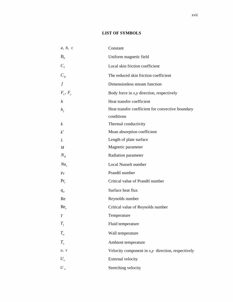
LIST OF SYMBOLS

, , ca b Constant

0B Uniform magnetic field

fC Local skin friction coefficient

fxC The reduced skin friction coefficient

f Dimensionless stream function

,x yF F Body force in x,y direction, respectively

h Heat transfer coefficient

fh Heat transfer coefficient for convective boundary

conditions

k Thermal conductivity

k Mean absorption coefficient

L Length of plate surface

M Magnetic parameter

RN Radiation parameter

xNu Local Nusselt number

Pr Prandtl number

Prc Critical value of Prandtl number

wq Surface heat flux

Re Reynolds number

Rex Critical value of Reynolds number

T Temperature

fT Fluid temperature

wT Wall temperature

T Ambient temperature

,u v Velocity component in x,y direction, respectively

eU External velocity

wU Stretching velocity

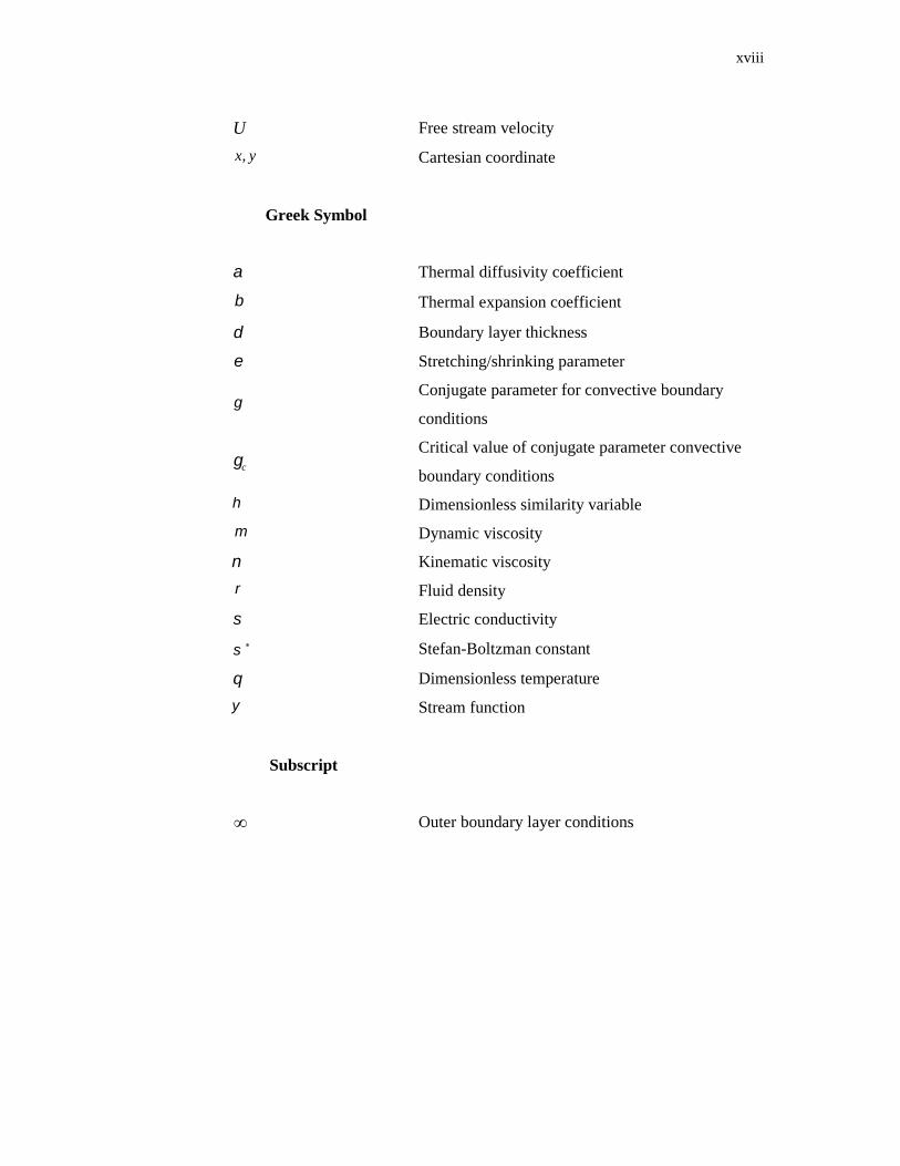
xviii

U Free stream velocity

,x y Cartesian coordinate

Greek Symbol

Thermal diffusivity coefficient

Thermal expansion coefficient

Boundary layer thickness

Stretching/shrinking parameter

Conjugate parameter for convective boundary

conditions

cCritical value of conjugate parameter convective

boundary conditions

Dimensionless similarity variable

Dynamic viscosity

Kinematic viscosity

Fluid density

Electric conductivity

Stefan-Boltzman constant

Dimensionless temperature

Stream function

Subscript

Outer boundary layer conditions

xix

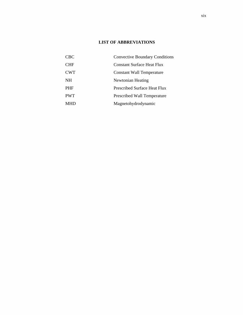
LIST OF ABBREVIATIONS

CBC Convective Boundary Conditions

CHF Constant Surface Heat Flux

CWT Constant Wall Temperature

NH Newtonian Heating

PHF Prescribed Surface Heat Flux

PWT Prescribed Wall Temperature

MHD Magnetohydrodynamic

CHAPTER 1

PRELIMINARIES

1.1 INTRODUCTION

Heat transfer is defined as the thermal energy transfer from a hotter object to a

cooler object. The transition can be made by conduction, radiation and convection. Heat

transfer by direct molecular contact which takes place without significant molecules

being moved in solids is called conduction. Conduction heat transfer can also take place

through direct contact of two bodies with different temperatures. Radiation heat transfer

takes place by the transition of heat through electromagnetic waves. Electromagnetic

waves can pass through a vacuum and also go through materials. In this study,

convection heat transfer will be considered. The transition of heat from one place to

another, through the physical movement of fluids and which, usually takes place

between a solid surface and fluid molecules through physical contact. Liquids and gases

are fervently used for dominant form of heat transfer. The convective mode of heat

transfer basically occurs into three elementary processes, which are free, forced and

mixed convection (Baehr and Stephan, 1994).

Forced convection happens when fluid motion is generated mechanically by

external forced like a fan, blower, nozzle or jet. Fluid motion related to a surface can be

generated by moving an object, such as a missile, through a fluid. Otherwise, the free

convection happens when the fluid motion is generated by gravitational field.

Occurrence of free convection requires fluid density change. In free convection,

temperature changes are primarily due to variations in density. Fluid flow and heat

transfer link to each other because of this continuity process from buoyancy to a

difference in temperature. An increase in the rate of heat exchange normally uses forced

2

convection. Heat radiator systems and regulatory temperature systems in the body’s

circulatory system, are examples of forced convection (Merkin and Pop, 2011).

Convective heat transfer can also be classified as having either internal or

external flow. Free, forced and mixed convection processes may be divided into having

an external flow over immersed body such as flat plates, cylinder, sphere or an internal

flow in ducts such as pipes, channels and enclosures. The resultant flow can further be

categorized as laminar (stable) or turbulent (unstable) flow. Laminar flow is smooth,

with a particle of fluid moving steadily in a smooth line parallel to a surface, while on

the other hand, turbulent flow is described as chaotic of fluid moving unsteadily

(Incropera, 2011).

1.2 BOUNDARY LAYER THEORY

The Ludwig Prandtl (1875-1953) on August 1904, introduced and developed the

boundary layer theory which states that a thin layer (region) sticks to a surface that is

embedded in a fluid motion field. This region (thin layer) near the surface is called the

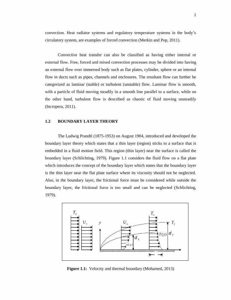
boundary layer (Schlichting, 1979). Figure 1.1 considers the fluid flow on a flat plate

which introduces the concept of the boundary layer which states that the boundary layer

is the thin layer near the flat plate surface where its viscosity should not be neglected.

Also, in the boundary layer, the frictional force must be considered while outside the

boundary layer, the frictional force is too small and can be neglected (Schlichting,

1979).

Figure 1.1: Velocity and thermal boundary (Mohamed, 2013)

T

yU U

T

fT

( )T y

( )u y

hT

3

Boundary layer equations can be derived by setting a few assumptions on the

boundary layer flow which are (Ahmad, 2009);

(i) The viscous effects are limited in a boundary layer only. The viscous effects

outside of the boundary layer are not important.

(ii) The boundary layer is smaller than the flat plate surface. If is the boundary

layer thickness and L is the length of flat plate surface, then 1L . Also,

x O L and y O .

(iii) The fluid obeys the no slip condition on a plate surface while the free stream

velocity at the outside of the boundary, when

, 0 0, ( ,0) 0, ( , )u x v x u x U and ( , ) 0v x where u and v are

velocity component in x and y direction, respectively, also U is free stream

velocity.

(iv) In the boundary layer, let ( )u O U .

1.3 BOUNDARY CONDITIONS

Generally, there are four common heating processes specifying the wall-to-

ambient temperature distributions (Merkin, 1994). These are the constant/prescribed

wall temperature (CWT/PWT), the constant/prescribed surface heat flux (CHF/PHF),

the Newtonian heating (NH) and the convective boundary conditions (CBC). In this

research, three types of boundary conditions are considered namely the prescribed wall

temperature (PWT), the prescribed surface heat flux (PHF) and the convective boundary

conditions (CBC). The precise mathematical form of the boundary conditions depends

on the specific problem.

1.3.1 Constant/Prescribed Wall Temperature

Usually, constant wall temperature and prescribed surface heat flux are applied

as boundary conditions in modelling natural convection flow. A constant wall

temperature is the thermal boundary condition which can be imposed at the inside wall

4

of the duct. For constant wall temperature, the temperature wT is constant, and boundary

condition is

20 , 1.1

x

LwT T T e

where T is the stream temperature assumed to be constant, 0T is a constant

which measures the rate of temperature increase along the sheet, L is the reference

length, In addition, the heat transfer coefficient in the laminar flow is strongly

dependent on the thermal boundary conditions. In laminar flow, the thermal boundary

layer has the biggest effects on the heat transfer coefficient. This boundary condition is

approximated in condensers, evaporators and liquids to the gas heat exchangers with

high velocity liquid flows (Kakac et al., 2013).

A number of researches on the boundary layer flow on exponentially stretching

with constant wall temperature have been done. For example, Sajid and Hayat (2008)

and Bidin and Nazar (2009) have solved analytically and numerically the effect of

radiation on the boundary layer flow and heat transfer over an exponentially stretching

sheet, respectively. Moreover, the effect of radiation on MHD flow and heat transfer on

an exponentially stretching sheet with constant wall temperature was solved

numerically and analytically by Ishak (2011) and Mabood et al. (2014), respectively.

Further, Ishak (2011) studied MHD flow and heat transfer over an exponentially

stretching sheet with radiation effects with constant wall temperature.

1.3.2 Constant/Prescribed Surface Heat Flux

For constant surface heat flux wq we first note that it is a simple matter to

determine the heat transfer coefficient and the boundary condition is

, 1.2w

Tk q

y

where0

( ) 2 x Lw wq x q a vLe is the variable surface heat flux and k is thermal

conductivity in the laminar flow over a flat plate, the heat transfer coefficient on a plate

5

is constantly maintained. There are many practical applications of constant surface heat

flux over the surface, for example; electric resistance heating, nuclear heating and in a

counter flows heat exchanger with equal thermal capacity rates. It is well-established

that convective heat transfer depends on the form of the thermal boundary conditions

imposed, with it being usual to take either a prescribed temperature or a prescribed

surface heat flux on the boundary surface. However, in many problems, particularly

those involving the cooling of electrical and nuclear components, the wall heat flux is

known (Shu and Pop, 1998).

In addition, heat transfer from a stretching surface with constant surface heat

flux is investigated by Shu and Pop (1998). Kumari et al. (1990) studied MHD flow

and heat transfer over a stretching sheet with prescribed wall temperature and heat flux.

Elbashbeshy and Aldawody (2010) studied the unsteady boundary layer flow and heat

transfer on a stretching sheet with heat flux in the presence of a heat source or sink.

Some other researchers also drew attention to investigate the boundary layer problem

with the case of constant surface heat flux. For example; Pavithra and Gireesha (2014)

numerically studied the unsteady boundary layer flow and heat transfer of a quiescent

fluid over an exponentially stretching sheet. Boundary layer flow and heat transfer over

an exponentially stretching porous sheet with the surface heat flux was investigated by

Mandal and Mukhopadhyay (2013).

1.3.3 Convective Boundary Conditions

Recent trends and demands in heat transfer engineering have forced researchers

to develop various new types of compact and light-weight heat transfer equipment with

superior performance and efficiency. Consider a fluid over a sheet along the x-axis. The

lower face of the sheet is in contact with another fluid a temperature fT . The sheet is

stretched and the fluid starts moving, this situation is called convective boundary

condition and the boundary condition is,

, 1.3f f

Tk h T T

y

6

where fT is the temperature of the hot fluid and fh is the heat transfer

coefficient. Due to the increase in the need for small-size units, the focus has been

casted on the effects of the interaction between developments of the thermal boundary

layer in both fluid streams, and of axial wall conduction, which usually affects heat

exchange performance (Salleh et al., 2010a, 2010b).

Since an early paper written by Luikov et al. (1971), many researchers have

studied the topics of conjugate heat transfer. In addition, the laminar flow and thermal

boundary layer over the flat plate in a uniform stream of fluid with convective boundary

condition was studied by Aziz (2009). Recently, Makinde and Aziz (2010) and Ishak

(2010) investigated the MHD mixed convection flow and steady laminar boundary layer

flow over a flat plate and vertical plate with convective boundary conditions,

respectively. Furthermore, the stagnation point flow and heat transfer over a

stretching/shrinking sheet with convective boundary condition was studied by Bachok

et al. (2013).

1.4 KELLER-BOX METHOD

Keller (1970) introduced the Keller-box to solve differential equation problems.

This method is implicit finite difference method used with Newton’s method for

linearization. It is suitable to solve parabolic partial differential equations and can also

be modified to solve a problem in any order. This method has been used widely since it

is flexible, fast, and easy to be programmed (Keller and Cebeci, 1972). The Keller-box

that is used in this study is based on the explanation by Na (1979) and Cebeci and

Cousteix (2005).

Kumari and Nath (1989), Nazar et al. (2002) and Ishak et al. (2008b) solved

boundary layer problems using the Keller-box method. Recently, other researchers had

used the Keller-box in solving the boundary layer problems including Salleh et al.

(2010a), Anwar et al. (2012) and Mohamed et al. (2013). A solution by the Keller-box

method involves the following four steps:

(i) The ordinary differential equation in reducing to a first-order system.

(ii) Writing the differential equations using the central differences.

7

(iii) The resulting algebraic equations from step 2 are linearised using Newton’s

method and rewritten in matrix-vector form.

(iv) The linear system is solved by using the block triadiagonal elimination

technique.

The detailed procedure for the Keller-box method will be discussed in Section 2.7.

1.5 STAGNATION POINT

Throughout the past decades, many researchers have been interested to

investigate the stagnation point flow because of the industrial scientific applicability.

For example, its application in the cooling of fans electronic devices, the cooling of

nuclear reactors during emergency shutdowns, the solar central receivers exposed to

wind currents, and hydrodynamic processes. At a stagnation point the speed of the fluid

is zero and all of the kinetic energy has been converted to internal energy and is added

to the local static enthalpy. In problems of fluid mechanics, the point in the flow field

where the local velocity of the fluid becomes zero is called a stagnation-point. This

point exists at the surface of the object where the fluid is brought to be at rest because of

a force exerted by the object. The Bernoulli equation shows that the total pressure in

terms of static pressure is called stagnation where the pressure is at maximum value

when the fluid velocity is zero (Jafar et al., 2011).

The stagnation point marks the location in the fluid flow where the approaching

flow divides and passes on both sides along a surface. The stagnation point flow exists

everywhere in the sense that, it certainly appears as a component of more complicated

flow fields. For example, in some situations, the flow is stagnated by a solid wall while

in others, there is a line interior to a homogeneous fluid domain or the interface between

two immiscible fluids (Tilley and Weidman, 1998). There are several types of

stagnations-point flows such as viscous or inviscid, steady or unsteady, two-

dimensional or three dimensional, orthogonal or oblique, and forward or rear (Lok,

2008). The two dimensional stagnation point which flows moving towards a stationary

plate was first studied by Hiemenz (1911), using similarity transformation to reduce the

Navier-Stokes equations to nonlinear ordinary differential equations.

8

1.6 RESEARCH OBJECTIVE

This research embarks on the following objectives:

(i) To analyse the mathematical models for the following problems:

a. The boundary layer stagnation point boundary layer flow and heat transfer

towards an exponentially stretching/shrinking sheet.

b. Effects of radiation on MHD boundary layer stagnation point flow towards

and exponentially stretching/shrinking sheet.

(ii) To carry out mathematical formulation and analyses of these problems.

(iii) To develop numerical algorithms for the computations of these problems.

(iv) To provide theoretical predictions and mathematical formulations that will help

to explain and verify experimental results in the future.

1.7 RESEARCH SCOPE

The flow is considered to be two-dimensional, Newtonian, incompressible and

laminar. The boundary conditions are prescribed wall temperature, prescribed surface

heat flux and convective boundary conditions. The Keller-box method with appropriate

numerical algorithm is used to solve the set of ordinary differential equations in related

problems.

1.8 LITERATURE REVIEW

1.8.1 Boundary Layer Stagnation Point Flow over a Stretching/Shrinking Sheet

During the last few decades, the viscous flow and heat transfer in the boundary

layer region due to a stretching sheet has attracted a considerable attention for many

researchers. In fact, it has several theoretical and technical applications in industrial

manufacturing processes. Some of the applications are the aerodynamic extrusion of

plastic sheets, hot rolling, wire drawing, glass-fibre production, the cooling and drying

of paper and textiles (Nadeem and Lee, 2012). The two-dimensional flow of a fluid near

a stagnation point is a classical problem in fluid mechanics. It was first examined by

9

Hiemenz (1911), who demonstrated that the Navier-Stokes equations governing flow

can be reduced to an ordinary differential equation using similarity transformation.

Later, Sakiadis (1961) introduced the concept of the boundary layer flow due to ambient

fluid on a continuous moving surface with a constant speed.

Then, Tsou et al. (1967) certified that the Sakiadis’s theoretical predictions for

Newtonian fluids by means of experimental studies. In this problem, the analytical and

experimental nature of the laminar and turbulent boundary layer flow and heat transfer

on a continuous moving surface was investigated. An exact solution of a steady two-

dimensional boundary layer flow over a linearly stretching surface was first considered

by Crane (1970). Gupta and Gupta (1977) investigated two-dimensional heat and mass

transfer over a stretching sheet subject to suction or blowing. In the same way, Chen

and Char (1988) studied the laminar boundary layer heat transfer flow over a linearly

stretching and moving plate with suction consideration, blowing and constant surface

heat flux. It was found that the thermal boundary layer thickness and wall temperature

reduces with increase in values of Prandtl number. The work of Hiemenz (1911) and

Crane (1970) was developed by Chiam (1994), who studied the stagnation point flow

towards a stretching surface.

The stagnation point flows have many applications in industrial science and

engineering. Because of that many researchers have examined the two-dimensional

stagnation point flow. Such as, Wang (2008) was the first to investigate the two-

dimensional and axisymmetric stagnation flow towards a shrinking sheet and analysed

using similarity transformation which reduces the Navier-Stokes equations to a set of

nonlinear ordinary differential equations. The results of this problem showed that the

unique solution exists for stretching/shrinking ( 1 ), as well as that the boundary

layer thickness becomes thinner as shrinking is decreased. Ishak et al. (2006) studied the

steady mixed convection boundary layer flow near the stagnation point flow over a

stretching vertical sheet immersed in an incompressible viscous fluid. In this study, the

Keller-box method was used to solve for the nonlinear ordinary differential. For

assisting flow, it showed that the value of the skin friction coefficient and the local

Nusselt number were increasing when the buoyancy parameter increases. Meanwhile,

by increasing the values of Pr, the local Nusselt number increases but the skin friction