Vol. 31 No. 2Diciembre 15, 2014

Sociedad Cubana de Físicay Facultad de Física,Universidad de La Habana

VOLVIENDO A LA CIMACuba en la XIX Olimpiada Iberoamericana de Física

Revista Cubana de FísicaImpresa: ISSN 0253 9268En línea: ISSN 2224 9268

La Revista Cubana de Física es una publicación arbitrada bi-anual auspiciada por la Sociedad Cubana de Física y la Facultad de Física de la Universidad de La Habana, que aparece los días 15 de julio y 15 de diciembre*The Revista Cubana de Fisica is a biannual, peer-reviewed journal released by the Cuban Physical Society and the Physics Faculty, University of Havana, on July 15th and December 15th *

59

61

66

71

75

83

90

96

98

101

103

106

REVISTA CUBANA DE FÍSICA Vol. 31, No. 2 (Diciembre 15, 2014)

EDITOR

E. ALTSHULER Facultad de Física, Universidad de la Habana 10400 La Habana, Cuba ealtshuler@fisica.uh.cu

EDICIÓN ELECTRÓNICA

R. CUAN Facultad de Física, Universidad de la Habana rcuan@fisica.uh.cu

J. J. GONZÁLEZ Facultad de Física, Universidad de la Habana jjgonzalez@fisica.uh.cu

EDITORES ASOCIADOS

A. J. BATISTA-LEYVA Instec, La Habana abatista@instec.cu

W. BIETENHOLZ Instituto de Ciencias Nucleares, UNAM wolbi@nucleares.unam.mx

G. DELGADO-BARRIO IMAFF-CSIC, Madrid gerardo@imaff.cfmac.csic.es

O. DÍAZ-RIZO Instec, La Habana odrizo@instec.cu

V. FAJER-ÁVILA SCF, La Habana vfajer@infomed.sld.cu

J. O. FOSSUM NTNU, Trondheim jon.fossum@ntnu.no

J.-P. GALAUP Lab.A. Cotton(CNRS) & Univ. Paris- Sud jean-pierre.galaup@lac.u-psud.fr

O. DE MELO Facultad de Física, Universidad de La Habana omelo@fisica.uh.cu

R. MULET Facultad de Física, Universidad de La Habana mulet@fisica.uh.cu

P. MUNÉ Facultad de Ciencias, Universidad de Oriente mune@cnt.uo.edu.cu

T. POESCHEL University Erlangen-Nuremberg thorsten.poeschel@fau.de

T. SHINBROT Rutgers University shinbrot@soemail.rutgers.edu

C. A. ZEN-VASCONCELOS Univ. Federal Rio Grade du Sul cesarzen@cesarzen.com

DISEÑO ERNESTO ANTÓN E. ALTSHULER

PORTADA: Delegación cubana a la XIX OibF. Desde la izquierda: E. Rodríguez-Pino, M. Romero (ORO), J. L. Gózalez (MENCIÓN), M. Ávila (BRONCE), H. Hernández y J. M. Mora. Foto: Carlos González

COORDENADASMi mensaje como presidenta de la Sociedad Cubana de FísicaM. Sánchez

ARTÍCULOS ORIGINALESDecay of perturbations in a quantum-dot-optical microcavity model [Decaimiento de las perturbaciones en un modelo de punto cuántico acoplado a una microcavidad óptica]A. González (Ed. J. P. Galaup)

Electrical characterizatons of CdTe/CdS polycrystalline thin film solar cells [Caracterizaciones eléctricas de celdas solares policristalinas a capas delgadas de CdTe/CdS]O. Almora-Rodríguez, L. Vaillant y A. Bosio (Ed. O. de Melo)

Mutagenesis and background neutron radiation [Mutagénesis y radiación de fondo de neutrones] A. González (Ed. E. Altshuler)

Optimización de un modelo para los planos CuO en el La2CuO4 [Optimization of a model for the CuO planes of La2CuO4]Y. Vielza y A. Cabo-Montes de Oca (Ed. E. Altshuler)

Estabilidad, observabilidad, controlabilidad y respuesta a frecuencias de un conmutador optoelectrónico de VO2, considerado como un dispositivo de entrada-salida en representaciones TF, SS y ZPK [Stability, observability, controlability and frequency response of a VO2 optoelectronic commuter, assuming it as an input-output devicein the TF, SS and ZPK representations]L. Benavides (Ed. E. Altshuler)

Estudio de superficies de aceros ferromagnéticos mediante microscopía holográfica digital por reflexión[Surface study of ferromagnetic steels by reflexion digital holographic microscopy]G. Moreno, J. Ricardo, F. Palacios, M. Muramatsu, L. F. Gomes, G. Palacios, J. L.Valin y Y. Marzo (Ed. V. Fajer)

COMUNICACIONES ORIGINALESTransverse magnetoresistance in BSSCO-Ag multi-filamentary tapes[Magnetorresistenca transversal en cintas multifilamentares de BSSCO-Ag]A. S. García-Gordillo, A. Borroto and E. Altshuler (Ed. P. Muné)

Energy storage power of antiferroelectric and relaxor ferroelectric ceramics [Poder de almacenamiento de energía de cerámicas antiferroeléctricas y ferroeléctricas relajadoras]A. Peláiz-Barranco, Y. González-Abreu, J.Wang y T. Yang (Ed. E. Altshuler)

The photobiological regime and oceanic primary production[El régimen fotobiológico y la producción oceánica primaria]L. Peñate, R. Cárdenas y S. Agusti (Eds. A. López & E. Altshuler)

La producción de entropía en la glicólisis del cáncer [Entropy production in the glycolysis of cancer]A. Guerra, L. Triana, S. Montero, R. Martín, J. Rieumont y J. M. Nieto-Villar (Ed. E. Altshuler)

An atomistic model of intermolecular interactions for simulations of liquid n-octane [Modelo atomístico de las interacciones intermoleculares para la simulación del líquido de n-octano]B. Rodríguez-Hernández, L. Uranga-Piña y A. Martínez-Mesa (Eds. A. Cabo & E. Altshuler)

*Titulo abreviado (ISO 4): Rev. Cub. Fis/ Abbreviated Title (ISO 4): Rev. Cub. Fis.

110

114

117

121

123

Molecular dynamics in hyperspherical coordinates [Dinámica molecular en coordenadas hiperesféricas]V. M. Freixas-Lemus, A. Martínez-Mesa y L. Uranga-Piña (Eds. A. Cabo & E. Altshuler)

PARA FÍSICOS Y NO-FÍSICOS And white light was created[Y se hizo la luz blanca]M. Sánchez (Ed. E. Altshuler)

NUESTRA FÍSICA EN NOTICIAS

COMENTARIOSCarta al Editor: Sobre el artículo “La cultura científica y la desfactualización de la enseñanza de la Física” [Letter to the Editor: on the paper “Scientific culture and the de-factualization of physics teaching”]F. Herrmann (Ed. E. Altshuler)

Carta al Editor: Respuesta al comentario de F. Herrmann[Letter to the Editor: reponse to F. Herrmann’s comment]A. González-Arias (Ed. E. Altshuler)

59

RE

VIS

TA C

UB

AN

A D

E F

ÍSIC

A,

Vol. 3

1,

No.

2 (

20

14

)CO

ORDE

NAD

AS

COORDENADAS

MI MENSAJE COMO PRESIDENTA DE LA SOCIEDAD CUBANA DE FÍSICA

En esta comunicación a los físicos de todo el país mi primer comentario está dirigido a los problemas que presenta hoy la enseñanza de nuestra ciencia en Cuba. Comencemos por el problema de la enseñanza básica, que tiene varios matices. En las escuelas hay dificultades que van desde la falta de materiales, hasta el espacio físico y la ausencia de laboratorios. Pero sobre todo, existe un problema de capacitación. Es obvia la falta de dominio y actualización de los maestros, y no hay medios de enseñanza, laboratorios o equipos modernos que puedan suplir la falta de conocimientos. Los problemas de formación básica que arrastran los jóvenes se aprecian en los resultados de los exámenes de ingreso a la educación superior. Luego, al ingresar en carreras en las que reciben asignaturas de Matemática, Física y Química dentro del currículo base, obtienen por lo general malos resultados en las evaluaciones, lo que resulta en altos índices de arrastre y repitencia.

Para ponerle fin a este problema, creo sinceramente que es imprescindible hacer una reforma educativa en el país. Hay que cambiar radicalmente la manera de impartir las ciencias básicas, utilizando nuevos métodos de enseñanza enfocados a desarrollar habilidades que potencien la capacidad de razonamiento y el análisis. Por otra parte, es necesario reforzar los preuniversitarios vocacionales y reinstaurar los exámenes especiales de ingreso a las carreras de ciencias básicas de la educación superior. En el caso de la capacitación, la sociedad cubana de Física (SCF), con el apoyo de la facultad de física de la Universidad de la Habana, se propone organizar escuelas anuales para contribuir a la superación de los profesores de enseñanza media. Un segundo tema íntimamente relacionado con el anterior es la necesidad de fomentar una cultura científica en nuestra sociedad. Para esto quiero proponer a nombre de la SCF realizar una campaña de divulgación científica en el país titulada Con-CIENCIA. Esta campaña estará dirigida a que la ciencia se vea como algo cotidiano, y a despertar la curiosidad y el interés en nuestros jóvenes y niños. Que en las calles, en el transporte colectivo, en los menús de las cafeterías, aparezcan mensajes y notas relacionados con la ciencia. Se trata de crear un ambiente que propicie la familiaridad con estos temas de una manera

ocurrente y atractiva. Ojalá logremos que la televisión y nuestros medios de prensa se involucren: es necesario que divulguen los temas científicos, de la misma manera en que se hace con el arte, el deporte, la economía y la política. Para poner un solo ejemplo de las actuales carencias, del 28 de septiembre al 4 de octubre de este año se celebró la XIX Olimpiada Iberoamericana de Física en Paraguay, donde nuestros muchachos obtuvieron una medalla de Oro, una de bronce y una mención. Este descastadísimo resultado solo se reseñó en la Revista Juventud Técnica. Sin embargo, si se obtiene una medalla de bronce en un evento deportivo incluso de menor categoría, los medios ofrecen una amplia cobertura a nivel nacional.

Hoy se habla cada vez más de la sociedad del conocimiento, pero la verdadera Sociedad del Conocimiento existirá cuando la ciencia forme parte de la cultura del país.

En las Universidades también faltan recursos, sobre todo para el desarrollo de la investigación. Existe, además, el problema del envejecimiento de los claustros y el del éxodo, sobre todo de los jóvenes, que emigran buscando mejores oportunidades en otros países. En particular, el prolongado proceso de reparación del edificio sede de la facultad de Física de la Universidad de la Habana, que ya lleva ocho años de duración, pone en peligro la sostenibilidad de la investigación y la formación de recursos humanos en el campo de la Física desarrollados durante los pasados 50 años en el país. Creo que la Academia de Ciencias de Cuba y las sociedades científicas deben tener una participación más activa en la solución de todos estos problemas.

Hablando ahora del funcionamiento interno de la Sociedad Cubana de Física, debo decir que en el mandato del presidente anterior se avanzó mucho en la integración de los físicos. En especial, se fortaleció el trabajo de los colectivos de físicos de las regiones central y oriental de la isla. Sin embargo, varias secciones se debilitaron: algunas, como la de Energías no convencionales y la de Protección radiológica, prácticamente han desaparecido. En este periodo me propongo reanimar el trabajo de todas las secciones y, en particular, rescatar estas dos.

En medio de todo esto, la SCF posee hoy una excelente representación y vínculo con las organizaciones relacionadas con la Física en la región. Presidimos el consejo directivo del Centro Latinoamericano de Física, y ocupamos el secretariado de la sociedad Iberoamericana de física (FEIASOFI).

Estamos en un momento donde los físicos cubanos han logrado una gran madurez. No puedo imaginar una mejor compañía para enfrentar los problemas que hoy nos afectan, a lo cual dedicaré toda la energía disponible durante mi mandato.

Rev. Cub. Fis. 31, 59 (2014)

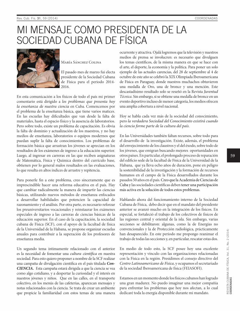
María Sánchez Colina

El pasado mes de marzo fui electa presidente de la Sociedad Cubana de Física para el periodo 2014-2016.

60

61

RE

VIS

TA C

UB

AN

A D

E F

ÍSIC

A,

Vol. 3

1,

No.

2 (

20

14

)AR

TÍCU

LOS

ORIG

INAL

ESE

d. J

.-P.

Gal

aup

ARTÍCULO ORIGINAL

DECAY OF PERTURBATIONS IN A QUANTUM-DOT-OPTICAL MICROCAVITY MODELDECAIMIENTO DE LAS PERTURBACIONES EN UN MODELO DE PUNTO CUÁNTICO ACOPLADO A UNA MICROCAVIDAD ÓPTICA

A. González

Instituto de Cibernetica, Matematica y Fsica, La Habana. agonzale@icimaf.cu

(Recibido 30/9/2013 ; Aceptado 18/6/2014)

The dynamics of small perturbations against the stationary density matrix of a pumped polariton system with only one photon polarization is studied. Depending on the way the system is pumped and probed, decay times ranging from 30 to 5000 ps are found. The large decay times under resonant pumping are related to a bottleneck effect in the decay of the excess (probe) populations of dark polariton states. No singular behaviour at the threshold for polariton lasing is observed.

Se estudia la evolución temporal de pequeñas perturbaciones alrededor de la matriz densidad estacionaria de un sistema bombeado de polaritones con sólo una polarización para los fotones. Dependiendo de la forma en que el sistema es bombeado y medido se obtienen tiempos de relajación en el rango de 30 a 5000 ps. Los tiempos grandes en régimen de bombeo resonante se relacionan con un efecto de embotellamiento en el decaimiento de las poblaciones en exceso de los estados polaritónicos oscuros. No se observa un comportamiento singular en el umbral del láser polaritónico.

PACS: 71.36.+c Polaritons, 78.47.Cd Time resolved luminescence, 42.55.Sa Microcavity and microdisk lasers

Polariton lasers are lasers without population inversion [1]. Coherence buildup in them is the result of the quasibosonic statistics of the polaritons, i.e. quasiparticles composed by electron-hole pairs from a quantum well strongly interacting with photons from a semiconductor microcavity. They share similarities with ordinary photon lasers and Bose-Einstein condensates [2, 3]. In these devices, the threshold power for lasing is 1 - 2 orders of magnitude lower than in ordinary lasers. Room-temperature polariton lasing has been recently reported [4].

Besides these promising characteristics, polaritons in microcavities provide an exceptional possibility for fundamental research. An example is the recent paper [5], where the authors seek for evidences of the Goldstone boson, which should appear in connection with the buildup of coherence in the polariton system. Indeed, in a cylindrical microcavity, the two (approximately) circular polarizations of the fundamental photon mode are related to two degenerate polariton “condensates”. The relative phase between the two photon polarizations acts as an order parameter. Phase fixing leads to a linear polarization [6], whose direction can be easily rotated (the Goldstone excitation). In paper [5], Ballarini et. al. study the changes in the PL response of a planar microcavity induced by small pulse perturbations of the pumping. They measure the lifetime of these perturbations, showing that it is much higher than the cavity decay time, and that it increases when the stationary pumping approaches the threshold for polariton lasing. These results are interpreted as a measurement of the lifetime of the Goldstone boson [7].

Recent experimental measurements of time-resolved PL in similar systems [8] reveal the importance of both the dynamics involving a single polarization, and the dynamics involving the two photon polarizations. On the other hand, a system with a single photon polarization - a single polariton condensate - could be realized by means of a strong magnetic field breaking the degeneracy between the “right-handed” and “left-handed” condensates.

In the present paper, I consider a model with a single photon polarization and explore how the way the system is pumped and probed influences the decay dynamics of the perturbations. I started from a scheme, sketched in Refs. [9, 10], in which pumping and photon losses in the polariton system are described by means of two terms in the master equation for the density matrix. The linearization of the master equation around the stationary solution leads to a system of equations with a source term for the small perturbations. The way the system is pumped determines the small-oscillation modes of these equations, whereas the way the system is probed determines which of the eigenmodes are excited. In an oversimplified model, with very strong exciton-photon coupling, I found decay times from 30 to 5000 ps, with no singular behaviour at the polariton lasing threshold. The large decay times correspond to eigenmodes involving the excitation of dark polariton states which, under resonant pumping, exhibit a bottleneck effect. In this sense, our results show that large decay times may not necessarily be connected with the lifetime of a Goldstone boson.

Rev. Cub. Fis. 31, 61 (2014)

62

RE

VIS

TA C

UB

AN

A D

E F

ÍSIC

A,

Vol. 3

1,

No.

2 (

20

14

)AR

TÍCU

LOS

ORIG

INAL

ESE

d. J

.-P.

Gal

aup

The starting point is a simple expression for the stationary spectral function, S(ω), describing the PL emission along the cavity symmetry axis, Eq. (19) of Ref. [11]:

S(ω) =1

π

∑I,J

|〈I|a|J〉|2ρ(∞)J ΓIJ

Γ2IJ + (ωIJ − ω)2

.

(1)

The magnitudes ΓIJ (linewidhts) and ωIJ = (EJ − EI )/ depend only on the many-polariton wavefunctions and energies, and the system parameters, P (pumping rate), and κ = 0.1 ps−1 (photon losses rate). ⟨I|a|J⟩ are the matrix elements of the photon annihilation operator between the many-polariton wavefunctions |J⟩ and |I⟩.

In our model, describing a many-exciton quantum dot strongly interacting with the lowest photon mode of a microcavity [11], the wavefunctions and energies, and from them ΓIJ , ωIJ, and ⟨I|a|J⟩, are obtained by numerically diagonalizing the electron-hole-photon Hamiltonian. On the other hand, the stationary solutions, should be obtained from the master equation for the occupations (coherences are three orders of magnitude smaller [10] and will be neglected):

dρIdt

= κ∑J

|〈I|a|J〉|2ρJ − κ ρI∑J

|〈J |a|I〉|2

+∑

Npol(J)=Npol(I)−1

ρJ PJI

− ρI∑

Npol(J)=Npol(I)+1

PIJ .

(2)

Npol(J) is the polariton number (number of electron-hole pairs plus number of photons, which is a conserved quantity) of state |J⟩, and PJI is the pumping rate from state J to state I. Notice that Eqs. (2) depends only on κ, P, and the matrix elements ⟨I|a|J⟩. These equations are linearly dependent, which expresses the conservation of probability:

∑I

ρI = 1. (3)

The stationary solutions, ρI(∞), are obtained by making

the l.h.s. of Eqs. (2) equal to zero, and complementing this homogeneous linear system with the normalization condition, Eq. (3).

Under a small perturbation of the pumping rate, δP(t), there is a variation of the density matrix, δρ(t), and a variation of the spectral function:

δS(ω, t) =1

π

∑I,J

|〈I|a|J〉|2 δρJ(t) ΓIJ

Γ2IJ + (ωIJ − ω)2

.

(4)

The response, δρI, to the pulsed perturbation δP(t) satisfies the linear system obtained by varying Eqs. (2):

dδρIdt

= κ∑J

|〈I|a|J〉|2δρJ − |〈J |a|I〉|2δρI

+∑

Npol(J)=Npol(I)−1

(δρJ PJI + ρ

(∞)J δPJI(t)

)

−∑

Npol(J)=Npol(I)+1

(δρIPIJ + ρ

(∞)I δPIJ(t)

),

(5)

which should be complemented with: ∑I

δρI = 0. (6)

The structure of Eqs. (5) is the following: dδρ/dt = Aδρ + δP(t)Bρ(∞). The eigenvalues of matrix A are the small oscillation frequencies of the system, whereas the probe perturbation, matrix B, and the stationary density matrix conform the source term determining which oscillation modes are excited by the probe pulse.

0.0001 0.00012 0.00014 0.00016 0.000181489

1489.2

1489.4Po

sitio

n of

the

PL p

eak

(meV

)

0.0001 0.00012 0.00014 0.00016 0.00018

Pumping Rate (ps-1

)

1.1

1.15

1.2

1.25

1.3

1.35

2nd

Ord

er C

oher

ence

Fun

ctio

n

(a)

(b)

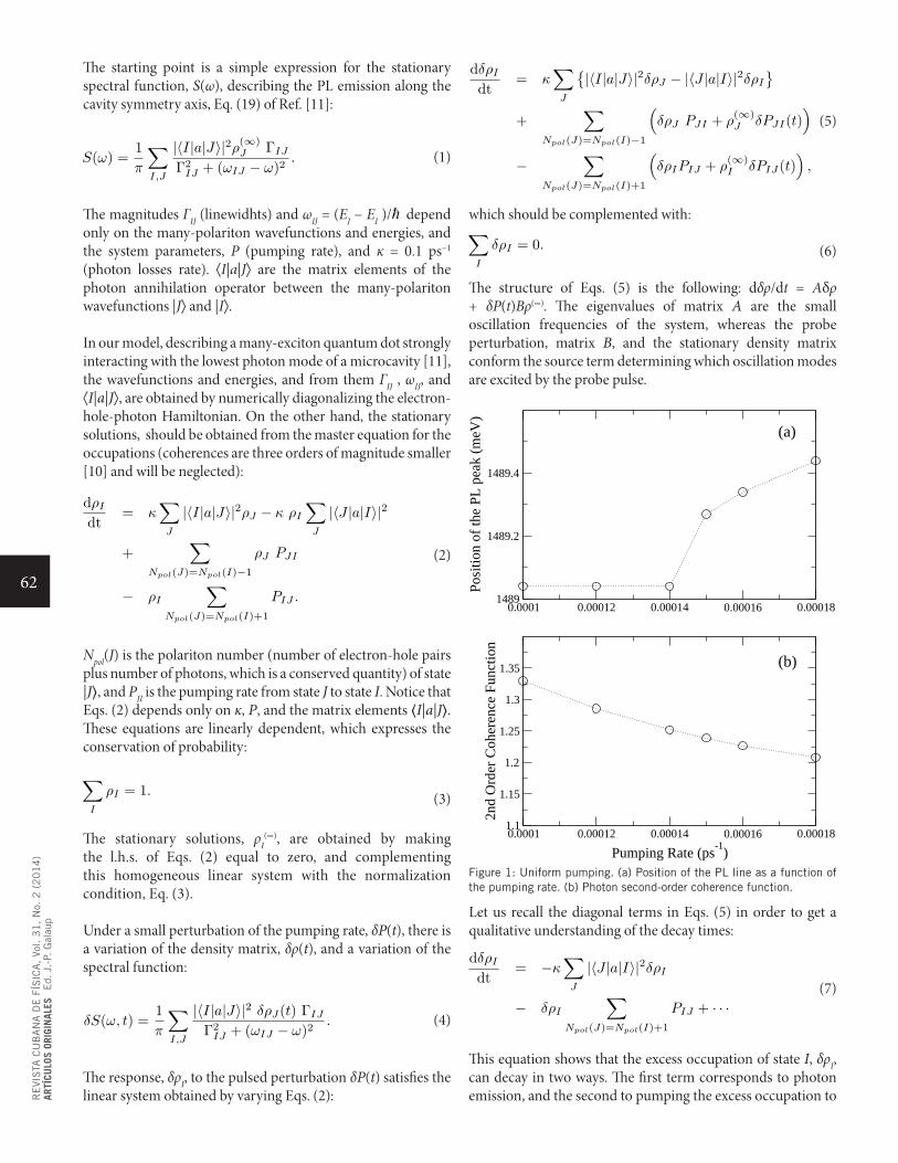
Figure 1: Uniform pumping. (a) Position of the PL line as a function of the pumping rate. (b) Photon second-order coherence function.

Let us recall the diagonal terms in Eqs. (5) in order to get a qualitative understanding of the decay times:

dδρIdt

= −κ∑J

|〈J |a|I〉|2δρI

− δρI∑

Npol(J)=Npol(I)+1

PIJ + · · ·

(7)

This equation shows that the excess occupation of state I, δρI, can decay in two ways. The first term corresponds to photon emission, and the second to pumping the excess occupation to

63

RE

VIS

TA C

UB

AN

A D

E F

ÍSIC

A,

Vol. 3

1,

No.

2 (

20

14

)AR

TÍCU

LOS

ORIG

INAL

ESE

d. J

.-P.

Gal

aup

a higher polariton state, J, which may further decay through photon emission. When the state I is dark, ΣJ|⟨J|a|I⟩|2 ≈ 0, only the second mechanism acts. If, in addition, δρI is not pumped to higher states because of selective pumping (PIJ ≈ 0), then the decay of δρI may take very long times. Below, we consider different regimes of pumping and probing the polariton system.

(a) Uniform pumping and uniform perturbation In this case, PIJ = P, and δPIJ(t) = δP (t). This situation seems to correspond to laser excitation energies well above the lower polariton branch, and perturbations at these higher energies.

I show in Fig. 1 the position of the main PL line as a function of the pumping rate, and the corresponding photon second-order coherence function, g(2)(0). The jump in the position of the line, and the values near one of g(2)(0) identify the threshold for polariton lasing at Pthr ≈ 0.00014 ps−1 in the model, where I use the following states in order to solve Eqs. (2) for the stationary density matrix: the vacuum (I =1), the 17 existing one-polariton states in the model (I =2−18), the 256 existing two-polariton states (I =19−274), and 256 states in each sector with 2 < Npol ≤ 10.

0 20 40 60 80 100

t (ps)0

0.0002

0.0004

0.0006

0.0008

0.001

Inte

grat

ed d

S (a

rb. u

nits

)

P=0.00012 ps-1

P=0.00014 ps-1

P=0.00015 ps-1

0 50 100 150 200

t (ps)

-2e-05

-1e-05

0

1e-05

2e-05

3e-05

Inte

grat

ed d

S (a

rb. u

nits

)

P=0.00012 ps-1

P=0.00014 ps-1

P=0.00015 ps-1

(a) Uniform Pumping, Uniform perturbation

(b) Uniform Pumping, Selective Perturbation

Figure 2: (Color online) Time evolution of the energy-integrated differential PL response, Eq. (9), under uniform pumping. (a) Uniform perturbation. (b) Selective perturbation.

I will study the decay dynamics of the probe for P values in the vicinity of Pthr . The probe pulse is taken in the following way:

δP (t) = 10−5 exp−(t− 1)2 ps−1, (8)

where t is given in ps. We find the δρI from Eqs. (5) and compute,

as in the experiment [5], the energy-integrated differential PL response:

δS(t) =∑J

δρJ(t)∑I

|〈I|a|J〉|2. (9)

The sum over I is restricted to states such that |EJ −EI − Eref| < δE, where δE = 2 meV, and the reference energy in the present case is Eref = 1489.2 meV.

0.02 0.03 0.04 0.05 0.06 0.07 0.081487.1

1487.2

1487.3

1487.4

1487.5

1487.6

Posi

tion

of th

e PL

pea

k (m

eV)

0.02 0.03 0.04 0.05 0.06 0.07 0.08

Pumping Rate (ps-1

)

1

1.02

1.04

1.06

1.08

1.12n

d or

der

Coh

eren

ce F

unct

ion

(a)

(b)

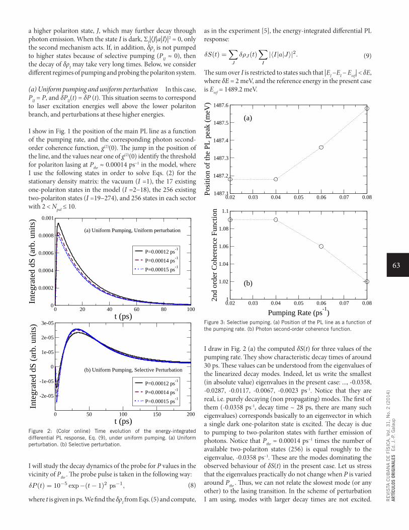
Figure 3: Selective pumping. (a) Position of the PL line as a function of the pumping rate. (b) Photon second-order coherence function.

I draw in Fig. 2 (a) the computed δS(t) for three values of the pumping rate. They show characteristic decay times of around 30 ps. These values can be understood from the eigenvalues of the linearized decay modes. Indeed, let us write the smallest (in absolute value) eigenvalues in the present case: ..., -0.0358, -0.0287, -0.0117, -0.0067, -0.0023 ps-1. Notice that they are real, i.e. purely decaying (non propagating) modes. The first of them (-0.0358 ps-1, decay time ~ 28 ps, there are many such eigenvalues) corresponds basically to an eigenvector in which a single dark one-polariton state is excited. The decay is due to pumping to two-polariton states with further emission of photons. Notice that Pthr = 0.00014 ps−1 times the number of available two-polariton states (256) is equal roughly to the eigenvalue, -0.0358 ps−1. These are the modes dominating the observed behaviour of δS(t) in the present case. Let us stress that the eigenvalues practically do not change when P is varied around Pthr . Thus, we can not relate the slowest mode (or any other) to the lasing transition. In the scheme of perturbation I am using, modes with larger decay times are not excited.

64

RE

VIS

TA C

UB

AN

A D

E F

ÍSIC

A,

Vol. 3

1,

No.

2 (

20

14

)AR

TÍCU

LOS

ORIG

INAL

ESE

d. J

.-P.

Gal

aup

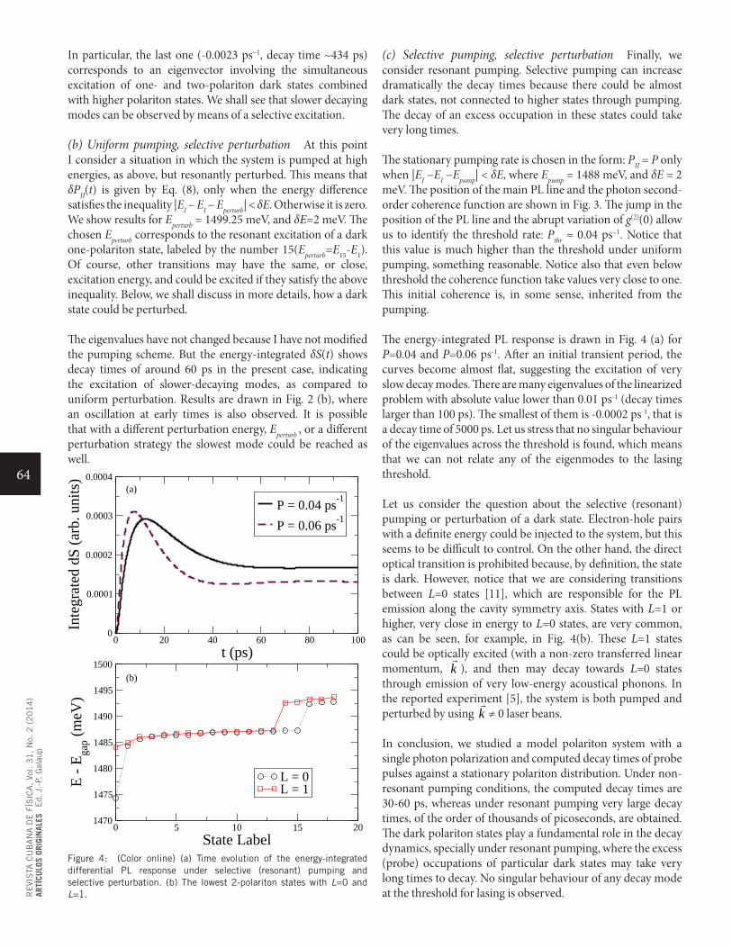
In particular, the last one (-0.0023 ps−1, decay time ~434 ps) corresponds to an eigenvector involving the simultaneous excitation of one- and two-polariton dark states combined with higher polariton states. We shall see that slower decaying modes can be observed by means of a selective excitation.

(b) Uniform pumping, selective perturbation At this point I consider a situation in which the system is pumped at high energies, as above, but resonantly perturbed. This means that δPIJ(t) is given by Eq. (8), only when the energy difference satisfies the inequality |EJ − EI − Eperturb| < δE. Otherwise it is zero. We show results for Eperturb = 1499.25 meV, and δE=2 meV. The chosen Eperturb corresponds to the resonant excitation of a dark one-polariton state, labeled by the number 15(Eperturb=E15-E1). Of course, other transitions may have the same, or close, excitation energy, and could be excited if they satisfy the above inequality. Below, we shall discuss in more details, how a dark state could be perturbed.

The eigenvalues have not changed because I have not modified the pumping scheme. But the energy-integrated δS(t) shows decay times of around 60 ps in the present case, indicating the excitation of slower-decaying modes, as compared to uniform perturbation. Results are drawn in Fig. 2 (b), where an oscillation at early times is also observed. It is possible that with a different perturbation energy, Eperturb , or a different perturbation strategy the slowest mode could be reached as well.

0 20 40 60 80 100

t (ps)0

0.0001

0.0002

0.0003

0.0004

Inte

grat

ed d

S (a

rb. u

nits

)

P = 0.04 ps-1

P = 0.06 ps-1

0 5 10 15 20

State Label1470

1475

1480

1485

1490

1495

1500

E -

Ega

p (m

eV)

L = 0L = 1

(a)

(b)

Figure 4: (Color online) (a) Time evolution of the energy-integrated differential PL response under selective (resonant) pumping and selective perturbation. (b) The lowest 2-polariton states with L=0 and L=1.

(c) Selective pumping, selective perturbation Finally, we consider resonant pumping. Selective pumping can increase dramatically the decay times because there could be almost dark states, not connected to higher states through pumping. The decay of an excess occupation in these states could take very long times. The stationary pumping rate is chosen in the form: PIJ = P only when |EJ −EI −Epump| < δE, where Epump = 1488 meV, and δE = 2 meV. The position of the main PL line and the photon second-order coherence function are shown in Fig. 3. The jump in the position of the PL line and the abrupt variation of g(2)(0) allow us to identify the threshold rate: Pthr ≈ 0.04 ps−1. Notice that this value is much higher than the threshold under uniform pumping, something reasonable. Notice also that even below threshold the coherence function take values very close to one. This initial coherence is, in some sense, inherited from the pumping.

The energy-integrated PL response is drawn in Fig. 4 (a) for P=0.04 and P=0.06 ps-1. After an initial transient period, the curves become almost flat, suggesting the excitation of very slow decay modes. There are many eigenvalues of the linearized problem with absolute value lower than 0.01 ps-1 (decay times larger than 100 ps). The smallest of them is -0.0002 ps-1, that is a decay time of 5000 ps. Let us stress that no singular behaviour of the eigenvalues across the threshold is found, which means that we can not relate any of the eigenmodes to the lasing threshold.

Let us consider the question about the selective (resonant) pumping or perturbation of a dark state. Electron-hole pairs with a definite energy could be injected to the system, but this seems to be difficult to control. On the other hand, the direct optical transition is prohibited because, by definition, the state is dark. However, notice that we are considering transitions between L=0 states [11], which are responsible for the PL emission along the cavity symmetry axis. States with L=1 or higher, very close in energy to L=0 states, are very common, as can be seen, for example, in Fig. 4(b). These L=1 states could be optically excited (with a non-zero transferred linear momentum, k

), and then may decay towards L=0 states through emission of very low-energy acoustical phonons. In the reported experiment [5], the system is both pumped and perturbed by using k

≠ 0 laser beans.

In conclusion, we studied a model polariton system with a single photon polarization and computed decay times of probe pulses against a stationary polariton distribution. Under non-resonant pumping conditions, the computed decay times are 30-60 ps, whereas under resonant pumping very large decay times, of the order of thousands of picoseconds, are obtained. The dark polariton states play a fundamental role in the decay dynamics, specially under resonant pumping, where the excess (probe) occupations of particular dark states may take very long times to decay. No singular behaviour of any decay mode at the threshold for lasing is observed.

65

RE

VIS

TA C

UB

AN

A D

E F

ÍSIC

A,

Vol. 3

1,

No.

2 (

20

14

)AR

TÍCU

LOS

ORIG

INAL

ESE

d. J

.-P.

Gal

aup

This work was supported by the Programa Nacional de Ciencias Basicas (Cuba) and the Caribbean Network for Quantum Mechanics, Particles and Fields (ICTP). The author is grateful to Alejandro Cabo and Alexey Kavokin for discussions.

[1] A. Imamoglu, R.J. Ram, S. Pau, and Y. Yamamoto, Phys. Rev. A 53, 4250 (1996). [2] H. Deng, G. Weihs, D. Snoke, J. Bloch, and Y. Yamamoto, Proc. Natl. Acad. Sci. 100, 15318 (2003). [3] D. Bajoni, P. Senellart, A. Lemaitre, and J. Bloch, Phys. Rev. B 76,201305 (R) (2007). [4] S. Christopoulos, G. Baldassarri Hoger von Hogersthal,

A.J.D. Grundy, et. al., Phys. Rev. Lett. 98, 126405 (2007). [5] D. Ballarini, D. Sanvitto, A. Amo, et. al., Phys. Rev. Lett. 102, 056402 (2009). [6] J. Kasprzak, R. Andre, Le Si Dang, et. al., Phys. Rev. B 75, 045326 (2007). [7] M. Wouters and I. Carusotto, Phys. Rev. B 75, 075332 (2007). [8] A.A. Demenev, A.A. Shchekin, A.V. Larionov, S.S. Gavrilov, and V.D. Kulakovskii, Phys. Rev. B 79, 165308 (2009). [9] H. Vinck-Posada, B.A. Rodriguez, P.S.S. Guimaraes, A. Cabo, and A. Gonzalez, Phys. Rev. Lett. 98, 167405 (2007). [10] C.A. Vera, A. Cabo, and A. Gonzalez, Phys. Rev. Lett. 102, 126404 (2009). [11] C.A. Vera, H. Vinck-Posada, and A. Gonzalez, Phys. Rev. B 80, 125302 (2009).

66

RE

VIS

TA C

UB

AN

A D

E F

ÍSIC

A,

Vol. 3

1,

No.

2 (

20

14

)AR

TÍCU

LOS

ORIG

INAL

ESE

d. O

. de

Mel

o

ARTÍCULO ORIGINAL

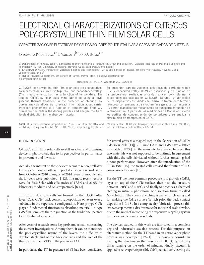
ELECTRICAL CHARACTERIZATIONS OF CdTe/CdS POLY-CRYSTALLINE THIN FILM SOLAR CELLS CARACTERIZACIONES ELÉCTRICAS DE CELDAS SOLARES POLICRISTALINAS A CAPAS DELGADAS DE CdTE/CdS

O. Almora-Rodríguez,a ‡ L. Vaillantb † and A. Bosioc *

a) Department of Physics, José A. Echeverría Higher Polytechnic Institute (ISPJAE) and ENERMAT Division, Institute of Materials Science and Technology (IMRE), University of Havana, Havana, Cuba; oalmora89@gmail.com‡b) ENERMAT Division, Institute of Materials Science and Technology (IMRE) and School of Physics, University of Havana, Havana, Cuba; vaillant@fisica.uh.cu†b) INFM- Physics Department, University of Parma, Parma, Italy; alessio.bosio@unipr.it*† corresponding author

(Recibido 21/3/2014; Aceptado 20/10/2014)

CdTe/CdS poly-crystalline thin film solar cells are characterized by means of dark current-voltage (I-V) and capacitance-voltage (C-V) measurements, both as a function of temperature. The studied CdTe/CdS solar cells were fabricated using a novel gaseous thermal treatment in the presence of chloride. I-V curves analysis allows us to extract information about carrier transport phenomena as a function of temperature. From C-V curves we can obtain the doping profiles and analyze the traps levels distribution in the absorber material.

Se presentan caracterizaciones eléctricas de corriente-voltaje (I-V) y capacidad voltaje (C-V) en oscuridad y en función de la temperatura, realizadas a celdas solares policristalinas a capas delgadas basadas en CdTe/CdS. Durante la fabricación de los dispositivos estudiados se utilizó un tratamiento térmico novedoso con presencia de cloro en fase gaseosa. La respuesta I-V permitió analizar los mecanismos de transporte en función de la temperatura. A partir de las mediciones de C-V se obtuvieron los perfiles de concentración de portadores y se analiza la distribución de trampas en el CdTe.

PACS: Thin films electrical properties of, 73.61.Ga; Thin film III-V and II-VI solar cells, 88.40.jm; Transport processes in thin films, 73.50.-h, 73.61.-r; Doping profiles, 61.72.U-, 81.70.Jb; Deep energy levels, 71.55.-I; Defect levels bulk matter, 71.55.-I.

INTRODUCTION

CdTe/CdS thin films solar cells are still an actual and promising device in photovoltaic due to its perspectives in performance improvement and low cost.

Actually, the interest on these devices seems to renew, well after ten years without an official reported efficiency record, since from October of 2010 to August of 2014 seven for modules and six for cells were publicized [1-12]. The most recent records were for First Solar with efficiencies of 17.5% and 21.0% for laboratory modules and cells respectively [8,12].

Thin film CdTe solar cells are formed by the TCO/ buffer layer/ CdS/ CdTe/ back contact superposition of layers over a substrate in the superstrate configuration. Here, p-type CdTe plays a fundamental function as absorbing material. n-type CdS film complete the p-n junction as the traditional partner for CdTe-based solar cell.

After years of research some key problems remain concerning the current investigations. Among them, it can be mentioned the poly-crystalline nature of the layers, the difficulty to develop stable and ohmic back contacts and the role of the thermal treatment (TT) in the presence of Cl.

In particular, the TT in presence of Cl has been considered

for several years as a magical step in the fabrication of CdTe/CdS solar cells [13][12]. Since CdTe and CdS have a lattice mismatch of 9.7% [14], the main interface created between this two materials was not supposed to be optimal. In agreement with this, the cells fabricated without further annealing had a poor performance. However, after the introduction of the TT in 1985 [15], the treated cells crossed the frontier of 11% conversion efficiency [16].

For the TT the most common procedure is to growth a CdCl2 layer on top of the CdTe surface, then heat the structure between 350°C and 400°C, and finally to practices a chemical etching in nitric + phosphoric acid solution (usually called NP solution). The chemical etching is made for cleaning and for making the CdTe surface Te-rich prior the back contact deposition [17, 18]. In a complete dry fabrication process this last wet step means a disadvantage for industrial scale develop, due to the need of introducing the expensive recycling system for the derived chemical residuals.

The devices studied in this work are fabricated in a complete dry and industrially scalable process. For this purpose, an alternative method for the TT based in an entire vapor phase process was developed [19-21]. This basically consists in heating the structure in the presence of HCF2Cl gas during times ranging on the order of minutes. Finally, vacuum is applied to re-evaporate possible CdCl2 remainders, leaving the

Rev. Cub. Fis. 31, 66 (2014)

67

RE

VIS

TA C

UB

AN

A D

E F

ÍSIC

A,

Vol. 3

1,

No.

2 (

20

14

)AR

TÍCU

LOS

ORIG

INAL

ESE

d. O

. de

Mel

o

CdTe surface ready for the back contact layer deposition.

In order to characterize CdTe/CdS solar cells treated with this alternative annealing the dark current-voltage (I-V) and capacitance-voltage (C-V) characteristics were considered, both as a function of temperature. Dark I-V curves allow us to investigate aspects related to the transport phenomena and C-V about the doping profiles and the presence of trap levels. These characterizations, mainly C-V, varying temperature are not frequently found in literature.

EXPERIMENTAL

The substrates used in the studied structure were soda-lime glasses of 2.5 cm2. Prior the cell fabrication the substrates are cleaned by submerging them in acetic acid, later in a solution of ethyl alcohol and nitric acid (with volumetric proportions of 1:3), and finally in a mixing of propanol and acetone. For the front contact fabrication the TCO was ITO and ZnO was introduced as the buffer layer. Both materials were deposited with direct current (DC) magnetron sputtering technique. For ITO deposition the substrate temperature was of 400°C - 450°C and the inert atmosphere was of 10-3 mbar of Ar with presence of oxygen in the chamber. The resulting film thickness was of about 1.0 μm. Similar parameters, but dispensing with the oxygen presence, were required for the ZnO layer.

Once the fabrication of the front contact was done, the structure was placed in the radio frequency (RF) magnetron sputtering system for the CdS film deposition. In this case were also used 10-3 mbar of Ar atmosphere, but this time with the inclusion of CHF3 in the atmosphere composition of the chamber. The substrate temperature was kept at 220°C and the thickness of the films was around 0.05 μm.

Subsequently, the CdTe layer fabrication was done by Close-Spaced Sublimation (CSS). In this step was used an atmosphere of pure Ar in the CSS chamber and the temperatures for the source and the substrate were about 570°C - 590°C and 510°C - 530°C, respectively. The resulting films presented thickness between 10 - 15 μm and columnar oriented grains with sizes near the 20 μm in the perpendicular sense of the light path.

For our novel TT the grown structure was located in the furnace chamber where the initial vacuum reached 10-6 mbar. After heating, the temperature was established around the 400°C. Later the compositions of HCF2Cl and Ar of 20 - 100 mbar and 800 - 900 mbar, respectively, were introduced in the chamber. Then the structure was treated during times between 2 and 10 minutes. After TT was practiced vacuum during 10 minutes for re-evaporate probable CdCl2 remainders.

The two back contact constituent layers (Sb2Te3 and Mo) were fabricated once more using the RF magnetron sputtering, with 10-3 mbar of Ar pressure and substrate temperature of 400°C. The thickness of the complete back contact film was evaluated in 0.1 μm. Following, the light soaking process was

practiced leaving the cells for several hours under 10 or more suns at temperatures higher than 100°C without observing degradation.

All the pressure measurements and controlling were performed by a Varian MultiGauge. The fabricated cells studied in this work reported efficiencies of 10.6-13.3% with active areas of 1.57 - 1.74 cm2. More information about the fabrication process can be found in [21].

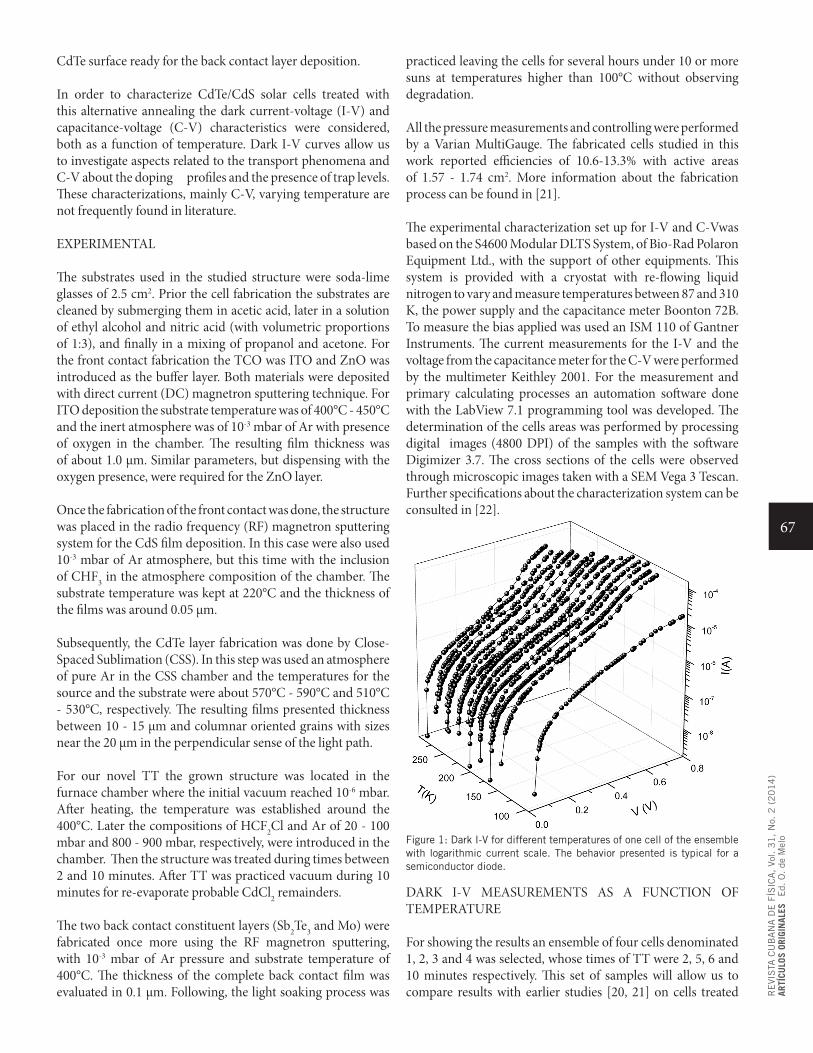
The experimental characterization set up for I-V and C-Vwas based on the S4600 Modular DLTS System, of Bio-Rad Polaron Equipment Ltd., with the support of other equipments. This system is provided with a cryostat with re-flowing liquid nitrogen to vary and measure temperatures between 87 and 310 K, the power supply and the capacitance meter Boonton 72B. To measure the bias applied was used an ISM 110 of Gantner Instruments. The current measurements for the I-V and the voltage from the capacitance meter for the C-V were performed by the multimeter Keithley 2001. For the measurement and primary calculating processes an automation software done with the LabView 7.1 programming tool was developed. The determination of the cells areas was performed by processing digital images (4800 DPI) of the samples with the software Digimizer 3.7. The cross sections of the cells were observed through microscopic images taken with a SEM Vega 3 Tescan. Further specifications about the characterization system can be consulted in [22].

Figure 1: Dark I-V for different temperatures of one cell of the ensemble with logarithmic current scale. The behavior presented is typical for a semiconductor diode.

DARK I-V MEASUREMENTS AS A FUNCTION OF TEMPERATURE

For showing the results an ensemble of four cells denominated 1, 2, 3 and 4 was selected, whose times of TT were 2, 5, 6 and 10 minutes respectively. This set of samples will allow us to compare results with earlier studies [20, 21] on cells treated

68

RE

VIS

TA C

UB

AN

A D

E F

ÍSIC

A,

Vol. 3

1,

No.

2 (

20

14

)AR

TÍCU

LOS

ORIG

INAL

ESE

d. O

. de

Mel

o

with approximately the half of pressure in the chamber.

Dark I-V characteristic behavior for the four cells presented the typical performance of a semiconductor diode [23], as it is shown in figure 1. The recombination-generation current region is displayed as the best defined, while the diffusion-current and high injection regions presented a slight trend to overlapping with the decrease of temperature.

Some differences in the evolution of the I-V curves with the temperature can be better appreciated in the linear scale, as it is shown in figure 2. The remarkable increase of the curves slope with temperature in the high voltage region suggests the decrease of series resistance (Rs) with the rise of temperature. The nature of this behavior responds to the predominant resistive element in the entire structure. In this sense the most likely factors to consider are the bulk of CdTe and the back contact. The bulk of CdTe occupy nearly the entire volume of the cell and its carrier concentration is significantly lower. On the other hand the back contact is known by its current rectifying effect for forward bias.

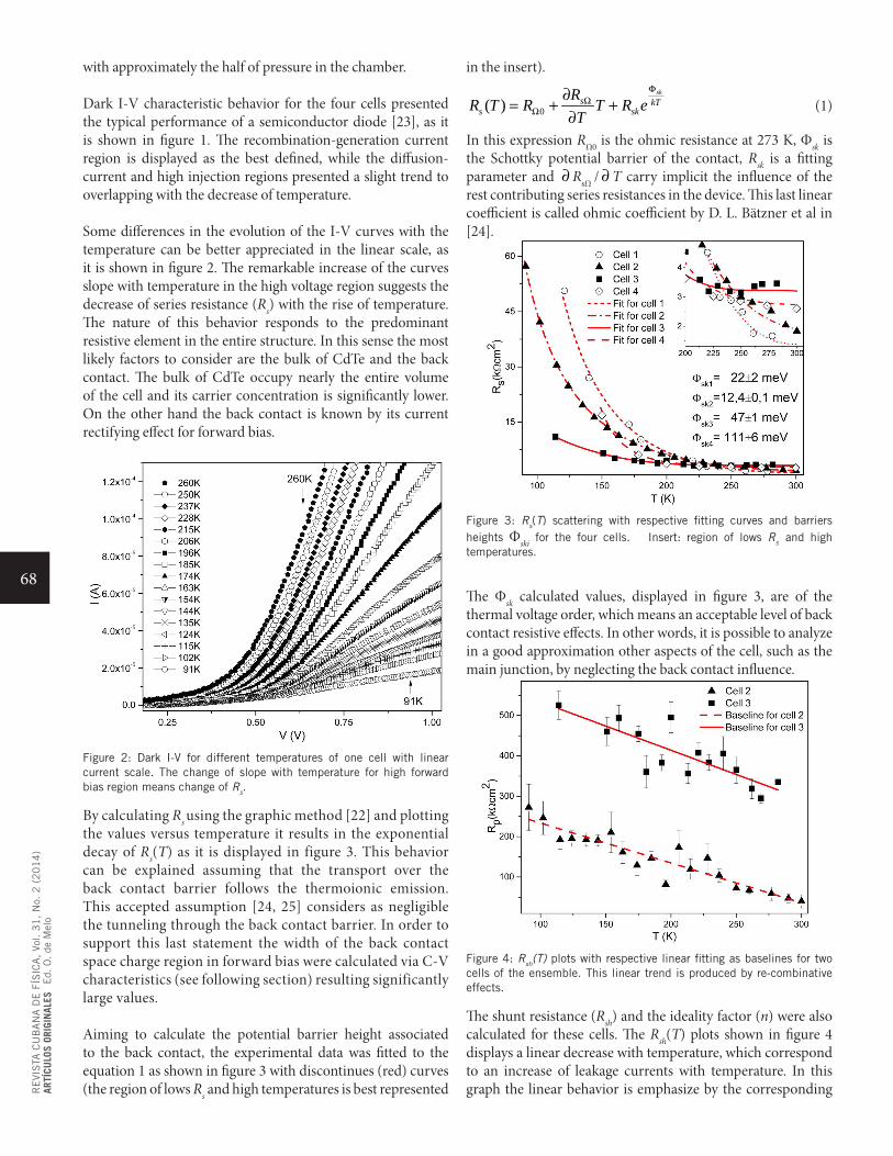
Figure 2: Dark I-V for different temperatures of one cell with linear current scale. The change of slope with temperature for high forward bias region means change of Rs.

By calculating Rs using the graphic method [22] and plotting the values versus temperature it results in the exponential decay of Rs(T) as it is displayed in figure 3. This behavior can be explained assuming that the transport over the back contact barrier follows the thermoionic emission. This accepted assumption [24, 25] considers as negligible the tunneling through the back contact barrier. In order to support this last statement the width of the back contact space charge region in forward bias were calculated via C-V characteristics (see following section) resulting significantly large values.

Aiming to calculate the potential barrier height associated to the back contact, the experimental data was fitted to the equation 1 as shown in figure 3 with discontinues (red) curves (the region of lows Rs and high temperatures is best represented

in the insert).

0( )sk

s kTs sk

RR T R T R e

T

ΦΩ

Ω∂

= + +∂

(1)

In this expression RΩ0 is the ohmic resistance at 273 K, Φsk is the Schottky potential barrier of the contact, Rsk is a fitting parameter and ∂ RsΩ / ∂ T carry implicit the influence of the rest contributing series resistances in the device. This last linear coefficient is called ohmic coefficient by D. L. Bätzner et al in [24].

Figure 3: Rs(T) scattering with respective fitting curves and barriers heights Φski for the four cells. Insert: region of lows Rs and high temperatures.

The Φsk calculated values, displayed in figure 3, are of the thermal voltage order, which means an acceptable level of back contact resistive effects. In other words, it is possible to analyze in a good approximation other aspects of the cell, such as the main junction, by neglecting the back contact influence.

Figure 4: Rsh(T) plots with respective linear fitting as baselines for two cells of the ensemble. This linear trend is produced by re-combinative effects.

The shunt resistance (Rsh) and the ideality factor (n) were also calculated for these cells. The Rsh(T) plots shown in figure 4 displays a linear decrease with temperature, which correspond to an increase of leakage currents with temperature. In this graph the linear behavior is emphasize by the corresponding

69

RE

VIS

TA C

UB

AN

A D

E F

ÍSIC

A,

Vol. 3

1,

No.

2 (

20

14

)AR

TÍCU

LOS

ORIG

INAL

ESE

d. O

. de

Mel

o

linear fitting curves that serve as baselines. This sort of tendency can be explained as a consequence of re-combinative effects in the low voltage region [26].

The Arrhenius plot displayed in figure 5 was elaborated for the analysis of n. Two remarkable characteristics predominate in that graph: the decrease of n with temperature and its values, higher than 2 practically for all of them. In CdTe/CdS devices these features suggest the prevailing of tunneling as a transport mechanism through the main junction [27]. A third characteristic is shaded in gray, which was the change in slope presented by all the cells around the 205 K; that is interpreted as a change in the main transport mechanisms at that temperature [24]. In our case this change may well be from the tunneling, at low temperatures, to recombination in the depletion region, at high temperatures [22].

Figure 5: Arrhenius plot of n for the four cells. The presented change of slope trend is shaded evidencing a change of main transport mechanisms.

C-V MEASUREMENTS AS A FUNCTION OF TEMPERATURE

C-V characteristics were performed always while decreasing the AC voltage and with a constant frequency of 1 MHz. These are aspects to attend due to the hysteresis effects always present in the capacitance studies [28].

The measurements are presented in the typical Mott-Schottky-plots, as displayed in figure 6 for one cell of the ensemble. The non-linearity of this curves evidence the strong presence of trap levels in the forbidden band of CdTe. Moreover, these kinds of irregularities make physically senseless the calculus of the majority carriers density and the built in potential by the model of the abrupt junction [23]. A correction to this model in such conditions has been proposed earlier [28] with the introduction of an intrinsic region inside the depletion region. The space charge region would have then a transition region where the majority carriers concentrations would vary between the intrinsic part, located next the juncture, and the concentration value in the border of the depletion region.

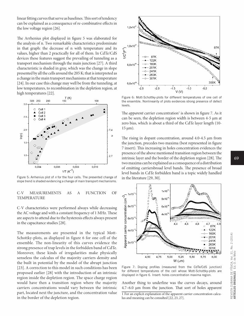
Figure 6: Mott-Schottky-plots for different temperatures of one cell of the ensemble. Nonlinearity of plots evidences strong presence of defect levels.

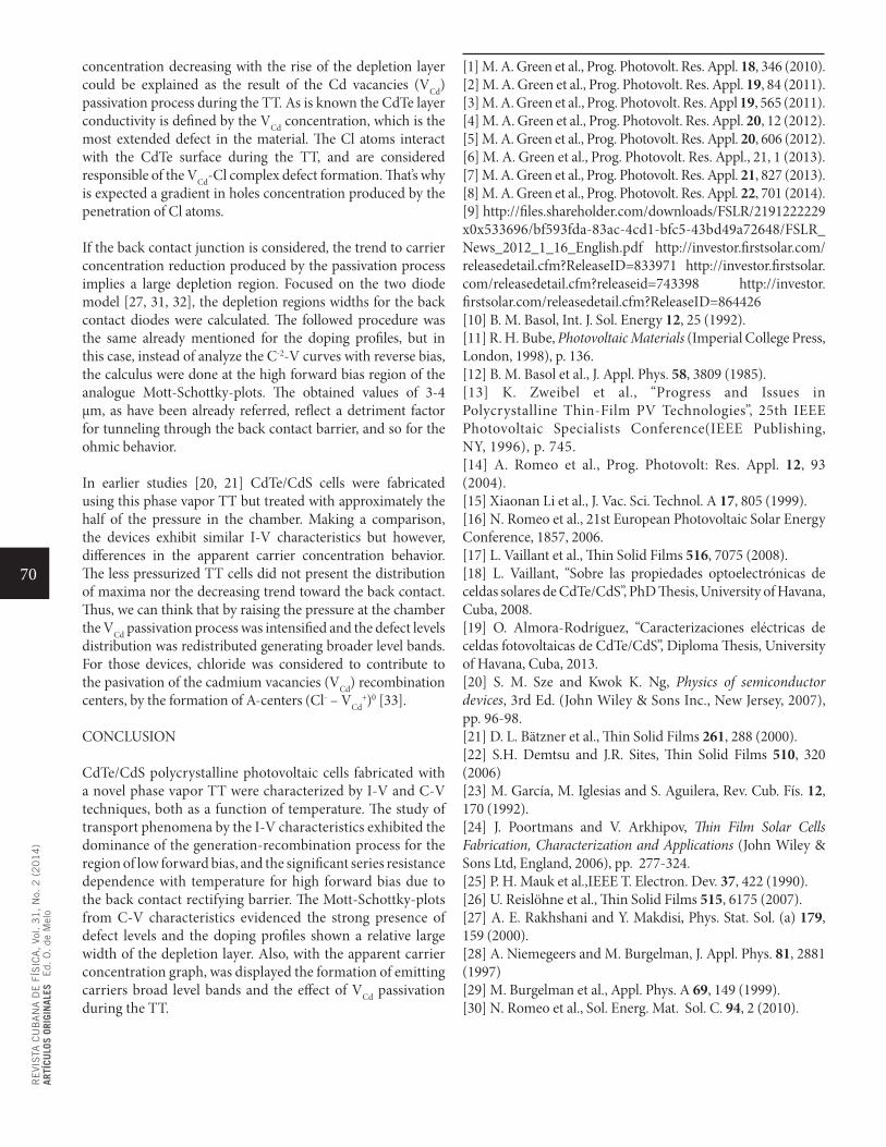
The apparent carrier concentration1 is shown in figure 7. As it can be seen, the depletion region width is between 4-5 μm at zero bias, which is about a third of the CdTe layer length (10-15 μm).

The rising in dopant concentration, around 4.0-4.5 μm from the junction, precedes two maxima (best represented in figure 7 insert). This increasing in holes concentration evidences the presence of the above mentioned transition region between the intrinsic layer and the border of the depletion region [28]. The two maxima can be explained as a consequence of a distribution of emitting carriersbroad level bands. The presence of broad level bands in CdTe forbidden band is a topic widely handled in the literature [29, 30].

Figure 7: Doping profiles (measured from the CdTe/CdS junction) for different temperatures of the cell whose Mott-Schottky-plots are displayed in figure 6. Insert: holes concentration maxima region.

Another thing to underline was the curves decays, around 4.7–6.0 μm from the junction. That sort of holes apparent 1 For an explicit explanation of the apparent carrier concentration calcu-lus and meaning can be consulted [22, 23, 27].

70

RE

VIS

TA C

UB

AN

A D

E F

ÍSIC

A,

Vol. 3

1,

No.

2 (

20

14

)AR

TÍCU

LOS

ORIG

INAL

ESE

d. O

. de

Mel

o

concentration decreasing with the rise of the depletion layer could be explained as the result of the Cd vacancies (VCd) passivation process during the TT. As is known the CdTe layer conductivity is defined by the VCd concentration, which is the most extended defect in the material. The Cl atoms interact with the CdTe surface during the TT, and are considered responsible of the VCd-Cl complex defect formation. That’s why is expected a gradient in holes concentration produced by the penetration of Cl atoms.

If the back contact junction is considered, the trend to carrier concentration reduction produced by the passivation process implies a large depletion region. Focused on the two diode model [27, 31, 32], the depletion regions widths for the back contact diodes were calculated. The followed procedure was the same already mentioned for the doping profiles, but in this case, instead of analyze the C-2-V curves with reverse bias, the calculus were done at the high forward bias region of the analogue Mott-Schottky-plots. The obtained values of 3-4 μm, as have been already referred, reflect a detriment factor for tunneling through the back contact barrier, and so for the ohmic behavior.

In earlier studies [20, 21] CdTe/CdS cells were fabricated using this phase vapor TT but treated with approximately the half of the pressure in the chamber. Making a comparison, the devices exhibit similar I-V characteristics but however, differences in the apparent carrier concentration behavior. The less pressurized TT cells did not present the distribution of maxima nor the decreasing trend toward the back contact. Thus, we can think that by raising the pressure at the chamber the VCd passivation process was intensified and the defect levels distribution was redistributed generating broader level bands. For those devices, chloride was considered to contribute to the pasivation of the cadmium vacancies (VCd) recombination centers, by the formation of A-centers (Cl- – VCd

+)0 [33].

CONCLUSION

CdTe/CdS polycrystalline photovoltaic cells fabricated with a novel phase vapor TT were characterized by I-V and C-V techniques, both as a function of temperature. The study of transport phenomena by the I-V characteristics exhibited the dominance of the generation-recombination process for the region of low forward bias, and the significant series resistance dependence with temperature for high forward bias due to the back contact rectifying barrier. The Mott-Schottky-plots from C-V characteristics evidenced the strong presence of defect levels and the doping profiles shown a relative large width of the depletion layer. Also, with the apparent carrier concentration graph, was displayed the formation of emitting carriers broad level bands and the effect of VCd passivation during the TT.

[1] M. A. Green et al., Prog. Photovolt. Res. Appl. 18, 346 (2010).[2] M. A. Green et al., Prog. Photovolt. Res. Appl. 19, 84 (2011).[3] M. A. Green et al., Prog. Photovolt. Res. Appl 19, 565 (2011).[4] M. A. Green et al., Prog. Photovolt. Res. Appl. 20, 12 (2012).[5] M. A. Green et al., Prog. Photovolt. Res. Appl. 20, 606 (2012).[6] M. A. Green et al., Prog. Photovolt. Res. Appl., 21, 1 (2013).[7] M. A. Green et al., Prog. Photovolt. Res. Appl. 21, 827 (2013).[8] M. A. Green et al., Prog. Photovolt. Res. Appl. 22, 701 (2014).[9] http://files.shareholder.com/downloads/FSLR/2191222229 x0x533696/bf593fda-83ac-4cd1-bfc5-43bd49a72648/FSLR_News_2012_1_16_English.pdf http://investor.firstsolar.com/releasedetail.cfm?ReleaseID=833971 http://investor.firstsolar.com/releasedetail.cfm?releaseid=743398 http://investor.firstsolar.com/releasedetail.cfm?ReleaseID=864426 [10] B. M. Basol, Int. J. Sol. Energy 12, 25 (1992).[11] R. H. Bube, Photovoltaic Materials (Imperial College Press, London, 1998), p. 136.[12] B. M. Basol et al., J. Appl. Phys. 58, 3809 (1985).[13] K. Zweibel et al., “Progress and Issues in Polycrystalline Thin-Film PV Technologies”, 25th IEEE Photovoltaic Specialists Conference(IEEE Publishing, NY, 1996), p. 745.[14] A. Romeo et al., Prog. Photovolt: Res. Appl. 12, 93 (2004).[15] Xiaonan Li et al., J. Vac. Sci. Technol. A 17, 805 (1999).[16] N. Romeo et al., 21st European Photovoltaic Solar Energy Conference, 1857, 2006.[17] L. Vaillant et al., Thin Solid Films 516, 7075 (2008).[18] L. Vaillant, “Sobre las propiedades optoelectrónicas de celdas solares de CdTe/CdS”, PhD Thesis, University of Havana, Cuba, 2008.[19] O. Almora-Rodríguez, “Caracterizaciones eléctricas de celdas fotovoltaicas de CdTe/CdS”, Diploma Thesis, University of Havana, Cuba, 2013.[20] S. M. Sze and Kwok K. Ng, Physics of semiconductor devices, 3rd Ed. (John Wiley & Sons Inc., New Jersey, 2007), pp. 96-98.[21] D. L. Bätzner et al., Thin Solid Films 261, 288 (2000).[22] S.H. Demtsu and J.R. Sites, Thin Solid Films 510, 320 (2006)[23] M. García, M. Iglesias and S. Aguilera, Rev. Cub. Fís. 12, 170 (1992).[24] J. Poortmans and V. Arkhipov, Thin Film Solar Cells Fabrication, Characterization and Applications (John Wiley & Sons Ltd, England, 2006), pp. 277-324.[25] P. H. Mauk et al.,IEEE T. Electron. Dev. 37, 422 (1990).[26] U. Reislöhne et al., Thin Solid Films 515, 6175 (2007).[27] A. E. Rakhshani and Y. Makdisi, Phys. Stat. Sol. (a) 179, 159 (2000).[28] A. Niemegeers and M. Burgelman, J. Appl. Phys. 81, 2881 (1997)[29] M. Burgelman et al., Appl. Phys. A 69, 149 (1999).[30] N. Romeo et al., Sol. Energ. Mat. Sol. C. 94, 2 (2010).

71

RE

VIS

TA C

UB

AN

A D

E F

ÍSIC

A,

Vol. 3

1,

No.

2 (

20

14

)AR

TÍCU

LOS

ORIG

INAL

ESE

d. E

. A

ltsh

uler

ARTÍCULO ORIGINAL

MUTAGENESIS AND BACKGROUND NEUTRON RADIATIONMUTAGÉNESIS Y RADIACIÓN DE FONDO DE NEUTRONES

A. González

Instituto de Cibernetica, Matematica y Fsica, La Habana. agonzale@icimaf.cu

(Recibido 19/6/2014 ; Aceptado 7/9/2014)

We suggest a possible correlation between the ionization events caused by the background neutron radiation and the experimental data on mutations with damage in the DNA repair mechanism, coming from the Long Term Evolution Experiment in E. Coli populations.

Se sugiere una posible correlación entre los eventos de ionización causados por la radiación de fondo de neutrones y los datos experimentales sobre mutaciones con daños en el mecanismo de reparación del ADN, provenientes del Experimento de evolución a largo plazo en poblaciones de E. Coli.

PACS: 61.80.Hg Neutron radiation effects , 87.53.-j Effects of ionizing radiation on biological systems, 87.23.Kg Dynamics of evolution

INTRODUCTION

In microelectronics, single failure events sporadically occur which, in some areas, like plane and space navigation, could have catastrophic consequences. Preliminary estimations [1] and more recent experiments [2] indicate a correlation between these events and the Background Neutron Radiation (BNR) [3]. The mechanism of failure is the collision of a neutron from the BNR with an atomic nucleus in the chip, leading to a shower of electrons and ions that locally changes the conductivity and shortcuts the device.

In the present paper, we suggest the BNR as a cause of genetic “fails” in living cells, that is one of the possible origins of the so called spontaneous mutations. Cells exposed to the shower of electrons and ions, caused by the collision of a neutron and a proton of water, could be anihilated or experience a permanent damage, in particular, a damage in the DNA. The frequency of such events is similar to the rate of appearance of mutations with damage in the DNA repair mechanism [4], as measured in the Long Term Evolution Experiment (LTEE), where E. Coli populations evolve under controlled conditions [5].

THE LTEE IN E. COLI POPULATIONS

The LTEE is an experiment conduced by Prof. R. Lenski and his group at the Michigan State University [5]. Each day, the bacteria undergo 6 - 7 generations of binary evolution. In a year, around 3400 generations occur. This means that, since the experiment started in 1988, it passed 60000 generations.

In the experiment, 12 populations of bacteria, with a common ancestor, independently evolve. Every day, 0.1 ml of the bacterial culture is serially transferred to 9.9 ml of a glucose solution, and mantained under controlled temperature until the next day.

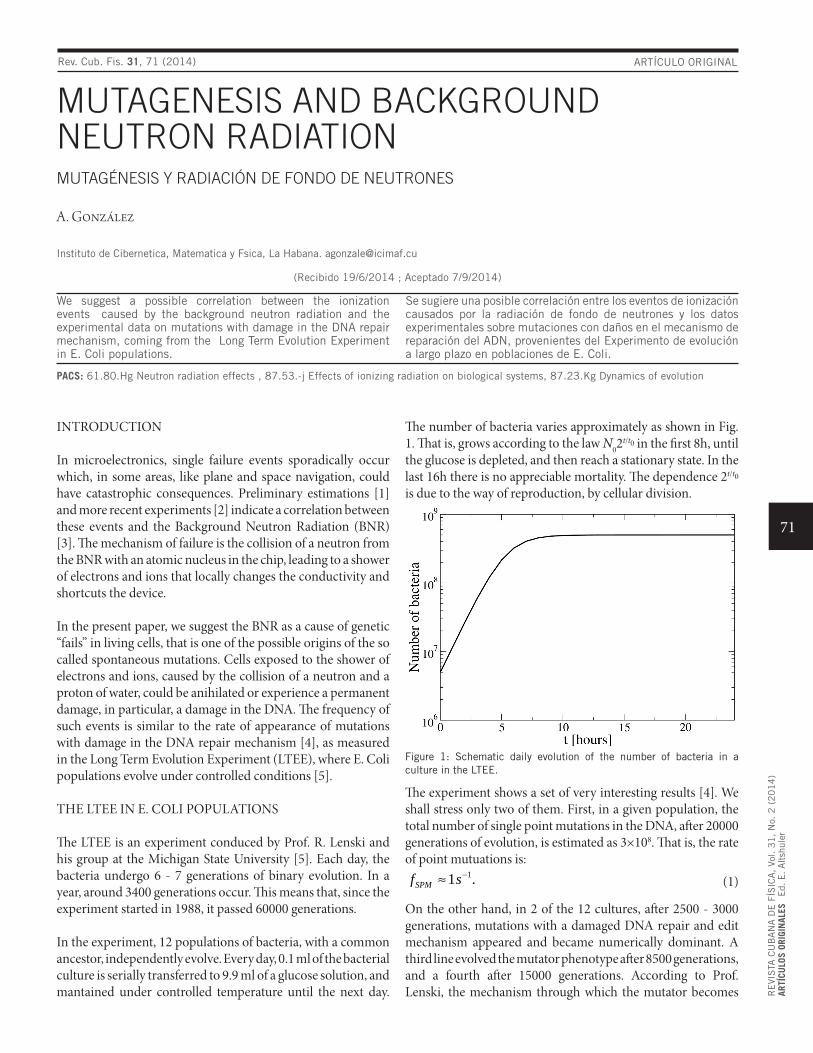
The number of bacteria varies approximately as shown in Fig. 1. That is, grows according to the law N02

t/t0 in the first 8h, until the glucose is depleted, and then reach a stationary state. In the last 16h there is no appreciable mortality. The dependence 2t/t0 is due to the way of reproduction, by cellular division.

Figure 1: Schematic daily evolution of the number of bacteria in a culture in the LTEE.

The experiment shows a set of very interesting results [4]. We shall stress only two of them. First, in a given population, the total number of single point mutations in the DNA, after 20000 generations of evolution, is estimated as 3×108. That is, the rate of point mutuations is:

11 .SPMf s−≈

(1)

On the other hand, in 2 of the 12 cultures, after 2500 - 3000 generations, mutations with a damaged DNA repair and edit mechanism appeared and became numerically dominant. A third line evolved the mutator phenotype after 8500 generations, and a fourth after 15000 generations. According to Prof. Lenski, the mechanism through which the mutator becomes

Rev. Cub. Fis. 31, 71 (2014)

72

RE

VIS

TA C

UB

AN

A D

E F

ÍSIC

A,

Vol. 3

1,

No.

2 (

20

14

)AR

TÍCU

LOS

ORIG

INAL

ESE

d. E

. A

ltsh

uler

numerically dominant is roughly the following. Once the mutation appears, the rate of spontaneous mutations increases 100 times, as compared with cells in which the DNA repair mechanism is not damaged. Thus, the mutator has a higher chance to generate the next winner and become dominant in a relatively short time scale, around 250 generations.

A second aspect, stressed by Prof. Lenski, is that mutations in which the DNA repair mechanism is damaged are “deleterious”, in the sense that a segment of the DNA is removed.

IONIZATION EVENTS CAUSED BY THE BNR

With regard to the BNR, we may assume that the cells live in pure water. Indeed, water is the main component of the solution, and the pH should be close to 7 in order to preserve life [6]. In these conditions, the important processes are the collisions between neutrons, from the BNR, and the Hydrogen nuclei (protons) of water. The ejected proton gives rise to a shower of ions and electrons that is extended approximately 0.1 mm along the proton trajectory.

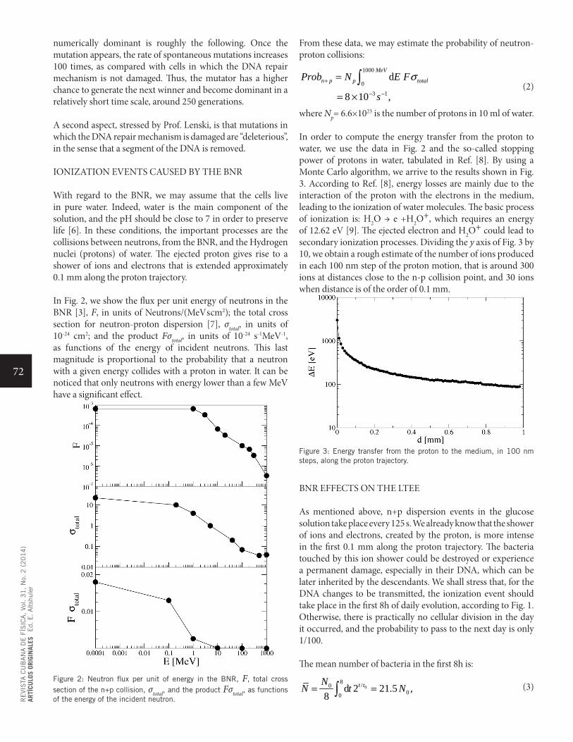
In Fig. 2, we show the flux per unit energy of neutrons in the BNR [3], F, in units of Neutrons/(MeV s cm2); the total cross section for neutron-proton dispersion [7], σtotal, in units of 10-24 cm2; and the product Fσtotal, in units of 10-24 s-1MeV-1, as functions of the energy of incident neutrons. This last magnitude is proportional to the probability that a neutron with a given energy collides with a proton in water. It can be noticed that only neutrons with energy lower than a few MeV have a significant effect.

Figure 2: Neutron flux per unit of energy in the BNR, F, total cross section of the n+p collision, σtotal, and the product Fσtotal, as functions of the energy of the incident neutron.

From these data, we may estimate the probability of neutron-proton collisions:

1000

03 1

d

8 10 ,

MeV

n p p totalProb N E F

s

σ+

− −

=

= ×∫

(2)

where Np= 6.6×1023 is the number of protons in 10 ml of water.

In order to compute the energy transfer from the proton to water, we use the data in Fig. 2 and the so-called stopping power of protons in water, tabulated in Ref. [8]. By using a Monte Carlo algorithm, we arrive to the results shown in Fig. 3. According to Ref. [8], energy losses are mainly due to the interaction of the proton with the electrons in the medium, leading to the ionization of water molecules. The basic process of ionization is: H2O → e +H2O

+, which requires an energy of 12.62 eV [9]. The ejected electron and H2O

+ could lead to secondary ionization processes. Dividing the y axis of Fig. 3 by 10, we obtain a rough estimate of the number of ions produced in each 100 nm step of the proton motion, that is around 300 ions at distances close to the n-p collision point, and 30 ions when distance is of the order of 0.1 mm.

Figure 3: Energy transfer from the proton to the medium, in 100 nm steps, along the proton trajectory.

BNR EFFECTS ON THE LTEE

As mentioned above, n+p dispersion events in the glucose solution take place every 125 s. We already know that the shower of ions and electrons, created by the proton, is more intense in the first 0.1 mm along the proton trajectory. The bacteria touched by this ion shower could be destroyed or experience a permanent damage, especially in their DNA, which can be later inherited by the descendants. We shall stress that, for the DNA changes to be transmitted, the ionization event should take place in the first 8h of daily evolution, according to Fig. 1. Otherwise, there is practically no cellular division in the day it occurred, and the probability to pass to the next day is only 1/100.

The mean number of bacteria in the first 8h is:

08 /0

00d 2 21.5 ,

8t tN

N t N= =∫

(3)

73

RE

VIS

TA C

UB

AN

A D

E F

ÍSIC

A,

Vol. 3

1,

No.

2 (

20

14

)AR

TÍCU

LOS

ORIG

INAL

ESE

d. E

. A

ltsh

uler

where N0 = 5×106 bacteria, and 28h/t0 =100. Each bacterium occupies a mean volume of around 10 cm3/(21.5 N0), that is, a cube with sides 45 μm long. In the first 0.1 mm =100 μm of the ion shower, only 2 such cubes could be allocated. The probability that the shower touches a bacterium is, thus:

2

3

Shower Volume 45 2 2 ,Cube Volume (45 )

l mmµ

µ×=

(4)

where l is the lateral dimension of the ion shower. l could be estimated from the Debye screening length of pure water:

1/20

2 ,2B

Dk T

nqλ

=

(5)

where kB denotes the Boltzman constant, ε ≈ 80 is the relative dielectric constant of water [10], q = 1 is the charge of the ions H+ y OH- in water, and n their concentration:

7 22 3

15 3

10 (3 10 molecules/cm )3 10 ions/cm .

n −= × ×= ×

(6)

Taking all these numbers together, we get λD= 500 nm = 0.5 μm. And putting l = λD in Eq. (4), we get a probability of 2.5×10-4. Notice that l is a magnitude of the same order of the E. Coli dimensions, thus the ion shower may cause strong effects on a bacterium.

We may compute the rate in which bacteria from a single population are touched by the BNR ionization events:

4 3 1

6 1

(2.5 10 ) (8 10 )

2 10 .BNRf s

s

− − −

− −

≈ × × ×

≈ × (7)

This number is very small, as compared with fSPM, Eq. (1). However, it is consistent with the frequency of deleterious mutations, with damage in the DNA repair mechanism, mentioned in section . Indeed, in Δt ~ 2400 generations ~1 year ~3×107 s, the BNR had a direct incidence on fBNR × Δt~60 bacteria. Some of them could have experienced damages in the DNA repair mechanism. The 100 times increase in the mutation rate could have given this subpopulation, after 100 - 600 generations, the possibility to generate beneficial mutations that would be fixed, allowing them to become numerically dominant. The fact that only 4 of 12 populations evolved in this way could be related to the probability ~1/3 that the BNR events take place in the first 8h of daily evolution.

Let us notice that we are assuming very fast BNR ionization events, as compared with the bacterial motion. Only those bacteria placed along the ion shower are affected by it. We may estimate the duration of such a event from:

01 ,τ

σ≈

(8)

where σ = 5.5 ×10-6 Coul/V s m is the conductivity of pure water [11]. That is, τ1 ≈ 10-4 s. A second estimate for the duration comes from the diffusion

constants of ions in water [12], D ≈103 μm/s. Taking λD = 0.5 μm as a characteristic dimension, results in:

24

2 2.5 10 .D sDλτ −≈ ≈ ×

(9)

In both cases, the times are of the order of 10-4 s. Taking into account that, at ambient temperatures, the typical speeds of bacterial motion are around 2 mm/s, only bacteria in contact with the ion shower, or very close to it, will be affected.

The fact that mutations with damage in the DNA repair mechanism are deleterious [4] is also consistent with the nature of BNR ionization processes. Indeed, the electron and ion shower is highly energetic and may produce such damages in the DNA, especially in the first steps after the n+p collision.

We shall compare the concentration of produced ions with the concentration of spontaneous ions in water, Eq. (6). In each of the first 100 nm steps, the ejected proton creates around 300 ions. The induced concentration is, thus:

16 32 3

300 1.2 10 ions/cm ,0.5 0.1 mindn

µ= = ×

× × (10)

that is, 4 times higher than n given in Ec. (6). The presence of ions in such high concentrations is also a strong mutagenic factor.

CONCLUDING REMARKS

In the present paper, we indicate a possible correlation between BNR ionization events and the LTEE observed rates of deleterious mutations with damages in the DNA repair and edit mechanism. In this way, we are indicating the probable origin of a class of “spontaneous” mutations.

The experimental confirmation of this possible correlation is plausible: restart the experiment by using fossils, and shield some of the evolving populations against the BNR. The shielded cultures should exhibit much lower rates for deleterious mutations with damages in the DNA repair mechanism. In around 1 - 2 years (2500 - 5000 generations), changes in mutation rates should be manifest.

On the other hand, a comment by Prof. Lenski [4] that some cancer cells also exhibit damages in the DNA repair mechanism, motivates us to rise the hypothesis about the BNR as one os the processes triggering cancer. Other events, like inhalation of radioactive Radon contained in air through breathing, are recognized carcinogens [13]. Defficient feeding, infectious proceeses, etc could be considered as conditions creating an evolutive pressure over the expossed cells, similar to the limited amount of glucose in the LTEE. Under these conditions, the BNR induced deleterious mutations, with damages in the DNA repair and edit mechanism, and the subsequent rise in the rate of spontaneous mutations, could allow the mutators to generate well adapted individuals that could become numerically dominant. In order to check this

74

RE

VIS

TA C

UB

AN

A D

E F

ÍSIC

A,

Vol. 3

1,

No.

2 (

20

14

)AR

TÍCU

LOS

ORIG

INAL

ESE

d. E

. A

ltsh

uler

hypothesis, a controlled experiment in animals could be designed, for example in mice, which are widely used as models of cancer in humans [14].

ACKNOWLEDGEMENTS

This work was supported by the Programa Nacional de Ciencias Basicas (Cuba) and the Caribbean Network for Quantum Mechanics, Particles and Fields (ICTP). The author acknowledges C. Ceballos for the information on the role of BNR in microelectronics, and E. Altshuler, A. Cabo, C. Cruz, G. Martín and E. Moreno for their comments and criticism.

[1] J.F. Ziegler, H.W. Curtis, H.P. Muhlfeld et. al., IBM J. Res. Dev. 40, 3 (1996). [2] T. Nakamura, M. Baba, E. Ibe, Y. Yahagi, H. Kameyama, Terrestrial neutron-induced soft errors in advanced memory devices, (Singapore, World Scientific, 2008); M. Nicolaidis, Ed., Soft errors in modern electronic systems, (Springer, New York, 2010). [3] M.S. Gordon, P. Goldhagen, K.P. Rodbell, et. al., IEEE T. Nuc. Sci. 51, 3427 (2004).

[4] R.E. Lenski, Phenotypic and genomic evolution during a 20000 generation experiment with the bacterium E. Coli, in J. Janick, Ed., Plant Breeding Reviews, Vol. 24, Part 2, page 225, 2004. [5] R. Lenski, Summary data from the long-term evolution experiment, http://myxo.css.msu.edu/ecoli/summdata.html [6] W. Boron, E.L. Boulpaep, Eds., Medical Physiology: A Cellular And Molecular Approach, (Elsevier, 2009). [7] J.W. Norbury, Nucleon-Nucleon Total Cross Section, NASA/TP-2008-215116. [8] PSTAR : Stopping Power and Range Tables for Protons, http://physics.nist.gov/PhysRefData/Star/Text/PSTAR.html [9] NIST data on the ionization potential of water, http://webbook.nist.gov/cgi/cbook.cgi? ID=C7732185&Mask=20 [10] M. Uematsu and E.U. Franck, J. Phys. Chem. Ref. Data 9, 129 (1980). [11] R.H. Shreiner and K.W. Pratt, Primary Standards and Standard Reference Materials for Electrolytic Conductivity, NIST Special Publication 260-142, 2004 Ed. [12] E.L. Cussler, Diffusion: Mass Transfer in Fluid Systems, (New York, Cambridge University Press, 1997). [13] National Research Council. Committee on Health Risks of Exposure to Radon: BEIR VI. Health Effects of Exposure to Radon. Washington, National Academy Press, 1999. [14] http://www.nih.gov/science/models/mouse/resources/hcc.html

75

RE

VIS

TA C

UB

AN

A D

E F

ÍSIC

A,

Vol. 3

1,

No.

2 (

20

14

)AR

TÍCU

LOS

ORIG

INAL

ESE

d. E

. A

ltsh

uler

ARTÍCULO ORIGINAL

OPTIMIZACIÓN DE UN MODELO PARA LOS PLANOS CuO EN EL La2CuO4OPTIMIZATION OF A MODEL FOR THE CuO PLANES IN La2CuO4

Y. Vielzaa ‡ y A. Cabo Montes de Ocab †

a) Facultad de Física, UH, Colina Universitaria, Vedado, La Habana, Cuba. yvielzadelacruz@gmail.com‡ b) Departamento de Física Teórica, Instituto de Cibernética, Matemática y Física, Calle E, No. 309, Vedado, La Habana, Cuba.cabo@icimaf.cu†† autor para la correspondencia

(Recibido 6/9/2014 ; Aceptado 8/10/2014)

Se extiende un estudio previo donde se consideró el efecto del dopaje con huecos en un modelo simple de las capas CuO2 del La2CuO4. Se reajustan los parámetros con el objetivo de fijar los valores del gap del material en 2 eV y su constante dieléctrica cercana a 21. De nuevo se obtienen indicios de una transición de fase “escondida” dentro del “domo” superconductor. La transición es de segundo orden y está asociada a la coincidencia energética de un estado básico aislante (AFA) con un estado excitado paramagnético que muestra un Pseudogap (PPG) en un punto crítico de concentración de huecos cercano a xc = 0.2. Se presenta la evolución con el dopaje de las bandas y las superficies de Fermi en las fases AFA y PPG. En la zona de bajo dopaje los huecos comienzan a ocupar los estados situados en la frontera de la zona de Brillouin, que en el estado AFA son los que cargan el antiferromagnetismo más intenso. Alrededor del dopaje crítico los resultados muestran que ambas fases tienden a coincidir en sus superficies de Fermi y los espectros de energía de los estados ocupados.

The results of a previous work, where it was considered the effect of hole doping on a simple model of the CuO2 planes in La2CuO4, are extended. The parameters are adjusted in order to fix the known values of the gap of 2 eV for this material and its dielectric constant of 21. We find again indications of a “hidden” phase transition inside the superconductor dome. The transition is a second order one, and is associated with an energetic coincidence of a ground insulator state (AFA) with an excited paramagnetic state showing a pseudogap (PPG), at a critical point of the hole concentration around xc = 0.2. We show the evolution as a function of doping of the band structures and the Fermi surface of the system in the phases AFA and PPG. In the zone of low doping, the holes begin to occupy the states located at the Brillouin zone, that in the AFA states have the strongest antiferromagnetic character. Around the critical doping the results show that in both phases the Fermi surfaces and the energy spectrum of the filled electronic states tend to coincide.

PACS: Cuprate superconductors 74.72.-h, Strongly correlated electron systems 71.27.+a, Metalinsulator transitions 71.30.+h, La-based cuprates 74.72.Dn, Theories and models of many electron systems 71.10.- w

I. INTRODUCCIÓN

En 1986 Georg Bednorz y Alex Müller, al investigar compuestos basados en el óxido de cobre, descubren los superconductores de alta temperatura crítica (HTSC por sus siglas en inglés) [1], generando un enorme interés en este tipo de materiales conocidos como “cupratos”. Estos sistemas cuentan con una estructura cristalina en la que se observan capas de óxidos de cobre que controlan el comportamiento del material ante el paso de la corriente eléctrica. En el estado normal la conducción eléctrica en estos planos es aproximadamente cien veces mayor que en la dirección perpendicular. Por esta razón se dice que, en cuanto a la conducción eléctrica, los cupratos son sistemas cuasi-bidimensionales [2]. Estos materiales tienen diferencias notables respecto a los superconductores que habían sido encontrados no sólo por su alta temperatura crítica, que no es explicable por la famosa teoría BCS, sino también debido a sus no convencionales propiedades físicas en la fase normal.

En contra de lo esperado a priori, los cupratos son aislantes de Mott y los electrones localizados se ordenan de forma

antiferromagnética. Un aislante de Mott es un sistema electrónico que se encuentra en una fase en la cual hay un gap en el espectro de energías de una partícula y este gap está generado por las fuertes correlaciones electrónicas y no por las características de la red como en los aislantes usuales. El paso de la corriente eléctrica en este tipo de materiales se inhibe para evitar que haya dos electrones en el mismo átomo ya que debido a la fuerte repulsión esto costaría mucha energía. Por su parte la fuerte tendencia de los cupratos a tener estados electrónicos ordenados se evidencia de las famosas fases tipo nemáticas o de stripes las cuales rompen alguna simetría espacial del sistema. Estas fases han sido intensamente estudiadas en superconductores de alta temperatura y actualmente pueden encontrarse en la literatura de distintos trabajos de resumen acerca del tema [3, 4]. La relación entre estos estados ordenados y los mecanismos que generan la superconductividad de alta temperatura son en la actualidad uno de los temas de mayor interés en la Física de la Materia Condensada.

Así, a pesar de la investigación intensiva y de muchas ideas prometedoras que buscan explicar la existencia de la

Rev. Cub. Fis. 31, 75 (2014)

76

RE

VIS

TA C

UB

AN

A D

E F

ÍSIC

A,

Vol. 3

1,

No.

2 (

20

14

)AR

TÍCU

LOS

ORIG

INAL

ESE

d. E

. A

ltsh

uler

superconductividad no convencional, aun no se ha logrado un consenso respecto a la tesis más apropiada. Una de las teorías que parece tener la base necesaria para alcanzar este fin está basada en el proceso de dopar con huecos un aislante de Mott, y en ella la superconductividad se genera directamente de la fuerte interacción repulsiva de los electrones.

Dentro de la amplia familia de cupratos se encuentra el La2CuO4 quien figura como uno de los compuestos más estudiados experimentalmente. Su simple estructura cristalina y regulada concentración de huecos sobre los planos bidimensionales CuO2, en un amplio régimen de dopaje, sugieren que una posible condensación de pares de huecos enlazados den lugar a propiedades de transporte superconductoras guiadas sobre las capas Cu-O.

Interesante resulta la variedad de fases de este material en la región de temperaturas cercanas al cero absoluto donde, en la medida que aumentamos la concentración de huecos, un estado AFA, existente a bajo dopaje, evoluciona hacia un estado superconductor y luego a un metal normal. No obstante, entre los aspectos más enigmáticos del diagrama de fases destaca una posible transición de fase cuántica dentro del Domo superconductor que se estima ocurre a cero temperatura en un punto crítico de concentración de huecos [5]. Resulta así necesario esclarecer los orígenes de la conducción en estos materiales y su evolución en la medida que se dopa el compuesto con vistas a descifrar la forma compleja que adopta su estructura. En particular nosotros estimamos que la existencia de estados ligados de huecos preformados en la fase AF aislante de Mott y su posterior condensación de Bose-Einstein muestran una ruta prometedora hacia la superconductividad.

Haciendo uso de un modelo de una banda resuelto en aproximación a HF, en las referencias [6, 7, 8] fue posible predecir la existencia tanto del estado aislante antiferromagnético como del estado de pseudogap en este material. Posteriormente en [13, 14], se introdujo el efecto de dopaje con huecos en dicho modelo, lo cual permitió describir varias propiedades de mucho interés del La2CuO4 a T = 0 K. Sin embargo, cabe subrayar que los resultados experimentales fijan el gap del estado básico AFA del La2CuO4 a 2.0 eV [9]y su constante diléctrica є a un valor cercano a 20 [10]. Los parámetros utilizados en [13], aunque fueron semejantes no coincidieron con esos valores (1.3 eV de gap y є aproximadamente igual a 10). De esa manera, la motivación central del presente trabajo la constituyó fijar con más precisión estas dos propiedades con vistas a establecer más apropiadamente dichos parámetros. En consecuencia, una vez optimizada las bases del modelo, también hicimos una corrección a los cálculos que incluyen el dopaje con huecos del compuesto. Como se describirá más adelante, en este proceso se prefijó nuevamente el ancho de la banda paramagnética obtenida de la solución HF, al valor del ancho 3.8 eV de la única banda que cruza el nivel de Fermi en los cálculos de bandas de Matheiss [11].

Describamos a continuación cómo procede la exposición. En la Sección 2 hacemos de inicio una revisión del modelo de una banda introducido en las referencias [6, 7, 8] y de su solución de campo medio. En esta sección también se realiza la fijación de los valores observados del gap (2 eV) y la constante dieléctrica (є = 21) del material. La solución de campo medio brinda entonces los estados aislante y de pseudogap a semillenado ( ausencia de dopaje). Finalmente, en la Sección 3 se investigan los estados que predice el modelo para las capas Cu-O en función del dopaje con huecos. Se estudia la evolución de la superficie de Fermi y de los estados uniparticulares HF en las fases AFA y PPG. Todo ello permite profundizar la argumentación dada en [13, 14] acerca de la existencia de una transición de fase cuántica dentro del Domo superconductor, tal como indican los datos experimentales [5].

II. MODELO DE TIGHT-BINDING DE LOS PLANOS CuO

En esta sección describiremos el modelo simplificado del plano cobre-oxígeno electrónico introducido en las referencias [6, 7, 8]. En la Figura 1, se ilustra el diagrama de bandas asociado al La2CuO4 obtenido mediante técnicas de LAPW (Linear Aumented Plane Waves) [4]. Describamos a partir de ese diagrama la construcción del modelo. Puede notarse que la última banda ocupada está semillena, lo cual predice un comportamiento metálico del material (hay una banda que atraviesa el nivel de Fermi en la Fig. 1). La forma de esta banda sugiere la validez de un esquema de electrones fuertemente ligados (TB) para el gas de electrones que la puebla. El electrón menos ligado al compuesto La2CuO4, es aquel que no se encuentra apareado en el Cu2+, que a diferencia de los O2− en el plano, no tiene su última capa (3d) cerrada. Estos electrones en un cuadro cualitativo, pueden estimarse como los que constituyen la única banda del material que corta el nivel de Fermi en los cálculos de la referencia [4]. Por esto es razonable considerar que esos electrones están fuertemente correlacionados a las celdas base CuO2 y con especial preferencia hacia los átomos de Cu correspondientes, asumida la completitud de capas del O2−. La anterior idea justifica tomar como la red asociada al modelo TB que daría lugar a la banda semillena de la referencia [4], como una red cuadrada de puntos coincidentes con los sitios Cu en el plano CuO2.

La presencia de todos los demás electrones que llenan las otras bandas en conjunto con las cargas nucleares que neutralizan la electrónica, juega un doble papel en el modelo. En primer lugar: como medio efectivo polarizable al cual asociamos cierta permitividad dieléctrica є que apantalla el campo producido por cualquier carga puntual extraña a él. En segundo lugar: por su distribución espacial y magnitud, se considera responsable en garantizar con su acción el orden periódico del sólido. Esto se modela a partir de suponer que esos electrones y cargas nucleares crean un potencial periódico confinante Wγ en la red puntual. El modelo se completa considerando las interacciones internas del gas electrónico que semillena la banda considerada y además su interacción con el excedente de cargas (jellium) que los neutraliza Fb. A este lo modelamos como una distribución

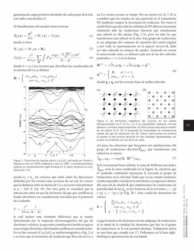
77

RE

VIS

TA C

UB

AN

A D

E F

ÍSIC

A,

Vol. 3

1,

No.

2 (

20

14

)AR

TÍCU

LOS

ORIG

INAL

ESE

d. E

. A

ltsh

uler

gaussiana de cargas positivas alrededor de cada punto de la red, con radio característico b.

El Hamiltoniano del modelo tiene la forma

H0(x) =p2

2m+Wγ(x) + Fb(x),

(1)

donde se tiene

Wγ(x) = Wγ(x+R), (2)

Fb(x) =e2

4πε0ε

∑R

∫d2y

exp(− (y−R)2

b2)/πb2

|x− y| ,

(3)

donde b << p y los vectores que describen las coordenadas de los átomos de Cu se definen

R =

(nx1p ex1 + nx2p ex2)con nx1 , nx2 ∈ Z

,

(4)

Figura 1: Estructura de bandas para el La2CuO4 calculada por Horsch y Stephan y cols. en 1993 y Matheiss y cols. en 1987. La banda semillena, predice un comportamiento tight-binding en el plano recíproco al CuO2 (dirección Γ-X).

siendo ex1 y ex2 los versores que están sobre las direcciones definidas por los vecinos más cercanos de esa red. Se conoce que la distancia entre un átomo de Cu y su vecino más próximo es p = 3,82 Å [18, 19]. Por otra parte se considera que la interacción entre un par de electrones del gas que semillena la banda electrónica en consideración está dada por el potencial de Coulomb:

V =e2

4πǫ0ǫ

1

|x− y| , (5)

la cual incluye una constante dieléctrica que se asume determinada por la respuesta electromagnética del gas de electrones y núcleos, ya que estos constituyen el medio en que se mueve el gas electrónico de la banda semillena en consideración. En su fase normal el La2CuO4 es antiferromagnético (Fig. 2 a) y se tiene que la invarianza de traslación que lleva de un Cu a

un Cu vecino cercano se rompe. Por ese motivo en [6, 7, 8] se consideró que los estados de una partícula en el tratamiento HF pudieran romper la invarianza de traslación. Por tanto el estado físico que describe los orbitales de HF debe ser invariante solamente ante las traslaciones discretas que transforman una subred en ella misma (Fig. 2 b), pero no ante las que transformen una subred en la otra. Este grupo de traslaciones es un subgrupo del conjunto de simetrías del cristal original y por ende su representación en el espacio inverso k, debe ser más reducida en número de estados. Teniendo en cuenta lo mencionado antes, se definen cada una de las dos subredes puntuales r = 1 o 2 en la forma:

R(r) =√2n1pq1 +

√2n2pq2 + q(r),

(6)q(r) =

0, si r = 1,p ex1 , si r = 2,

donde q1 y q2 son los versores base de ambas subredes.

Figura 2: (a) Estructura magnética del La2CuO4 en sus planos bidimensionales Cu-O. El Cu y el O se representan mediante círculos abiertos y cerrados respectivamente. (b) Red puntual asociada al modelo de los planos Cu-O. En la búsqueda de propiedades de correlaciones fuertes del gas de electrones fue útil liberar restricciones de simetría al separar la red puntual absoluta en dos subredes representadas con puntos coincidentes con los sitios de cobre.

Así pues, las soluciones que buscamos son autofunciones del grupo de traslaciones discretas R(1)T , que transforman una subred en sí misma:

TR(1)φk,l = exp(ik ·R(1))φk,l. (7)

Si la red puntual fuese infinita, la zona de Brillouin asociada aR(1)T sería la zona sombreada en la Figura 3a, mientras que

el cuadrado continente representa la asociada al grupo de traslaciones en la red total. Dado que en un estudio numérico resulta imposible considerar la red infinita, escogeremos dentro ella una red de estados k que implementen las condiciones de periodicidad de las ϕk,l

en las fronteras de la red total x1 = −Lp y Lp, x2 = −Lp y Lp (Fig. 3b ). Esta condición determina los valores

k =

2πLp

(nx1ex1 + nx2ex2)

con nx1 , nx2 ∈ Z

y − L2 ≤ nx1 ± nx2 < L

2

.

Luego el número de elementos en este subgrupo de traslaciones es la mitad de la cantidad de elementos que hay en el grupo de traslaciones en la red puntual absoluta. Trabajemos ahora en una base que cumpla con (7). Definamos así la base tight-binding en aproximación de una banda

(a) (b)

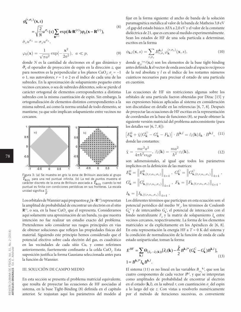
78

RE

VIS

TA C

UB

AN

A D

E F

ÍSIC

A,

Vol. 3

1,

No.

2 (

20

14

)AR

TÍCU

LOS

ORIG

INAL

ESE

d. E

. A

ltsh

uler

( )

( , )

( ) ( )0

( , )

2 ( ) exp( · ) ( ),

z

z

r

r

r r

s

u s iN

σ

σ

ϕ

ϕ= −∑k

R

x

k R x R

(8)

σzuσz = σzu

σz ,

ϕ0(x) =1√πa2

exp(− x2

2a2), a ≪ p,

(9)

donde N es la cantidad de electrones en el gas dinámico y ˆ zσ el operador de proyección de espín en la dirección z, que

para nosotros es la perpendicular a los planos CuO2; σz = −1 o 1, sus autovalores; r = 1 o 2 es el índice de cada una de las subredes. En la aproximación de solapamiento pequeño entre vecinos cercanos, o sea de subredes diferentes, solo se pierde el carácter ortogonal de elementos correspondientes a distintas subredes con la misma cuantización de espín. Sin embargo, la ortogonalización de elementos distintos correspondientes a la misma subred, así como la norma unidad de todo elemento, se mantiene, ya que solo implican solapamiento entre vecinos no cercanos.

Figura 3: (a) Se muestra en gris la zona de Brillouin asociada al grupo

R(1)T para una red puntual infinita. (b) La red de puntos muestra el carácter discreto de la zona de Brillouin asociada a R(1)T cuando la red puntual es finita con condiciones periódicas en sus fronteras. La escala unidad significa .

Los orbitales de Wannier aqui propuestos φ0(x−R(r)) representan la amplitud de probabilidad de encontrar un electrón en el sitio R(r), o sea, en la base CuO2 que el representa. Consideramos aquí solamente una aproximación de un banda, ya que nuestra intención no fue realizar un estudio exacto del problema. Pretendemos solo considerar sus rasgos principales en vías de obtener soluciones que reflejen las propiedades físicas del material. Siguiendo este principio hemos considerado que el potencial efectivo sobre cada electrón del gas, es cuadrático en las vecindades de cada sitio Cu, y como referimos anteriormente, fuertemente confinante a la celda CuO2. Esta suposición justifica la forma Gausiana seleccionada antes para la función de Wannier.

III. SOLUCIÓN DE CAMPO MEDIO

En esta sección se presenta el problema matricial equivalente, que resulta de proyectar las ecuaciones de HF asociadas al sistema, en la base Tight-Binding (8) definida en el capítulo anterior. Se reajustan aquí los parámetros del modelo al

fijar en la forma siguiente: el ancho de banda de la solución paramagnética metálica al valor de la banda de Matheiss 3,8 eV , el gap del estado básico AFA a 2,0 eV y el valor de la constante dieléctrica de 21, que es cercano al medido experimentalmente.Sean los estados de HF de una sola partícula a determinar, escritos en la forma

φk,l(x, s) =∑r,σz

Bk,lr,σz

ϕ(r,σz)k (x, s),

(10)

donde φk,l(r,σz)(x,s) son los elementos de la base tight-binding

antes definida, k el vector de onda asociado al espacio recíproco de la red absoluta y l es el índice de los restantes números cuánticos necesarios para precisar el estado de una partícula en cuestión.

Las ecuaciones de HF sin restricciones algunas sobre los orbitales de una partícula fueron obtenidas por Dirac [15] y sus expresiones básicas aplicadas al sistema en consideración son discutidase en detalle en las referencias [6, 7, 8]. Después de proyectar las ecuaciones de HF escritas en la representación de coordendas en la base de funciones (8), se puede obtener la siguiente versión matricial del problema autoconsistente (para los detalles ver [6, 7, 8]):[E0

k + χ(GCk −Gi

k − Fk)]·Bk,l = εl(k)Ik ·Bk,l,

(11)

donde las constantes:

χ =me2a2

4πh2ǫǫ0p, εl(k) =

ma2

h2εl(k),

(12)

son adimensionales, al igual que todos los parámetros implícitos en la definición de las matrices:

E0k =

∥∥∥E0k,(t,r,αz ,σz)

∥∥∥4×4

, GCk =

∥∥∥GCk,(t,r,αz ,σz)

∥∥∥4×4

,

Gik =

∥∥∥Gik,(t,r,αz ,σz)

∥∥∥4×4

, Fk =∥∥Fk,(t,r,αz ,σz)

∥∥4×4

,

Ik =∥∥Ik,(t,r,αz ,σz)

∥∥4×4

.

Los diferentes términos que participan en esta ecuación son: el potencial periódico del medio Wγ, los términos de Coulomb Gk

C y de intercambio Gki, el potencial de interacción con el

fondo neutralizante Fb y la matriz de solapamiento Ik entre vecinos cercanos, respectivamente. La forma de los elementos matriciales se da explícitamente en los Apéndices de [6, 8]. En esta representación la energía HF a T = 0 K del sistema y la condición de normalización de la función de onda de cada estado uniparticular, toman la forma:

, * ,( ( ))

,, * ,

[ ( ) ( ) ],2

1 .

F l

HF l C i ll

ll l

E B G G B

B I B

ε εχε− −

=

= Θ −∑ k kk k k

kk k

k

k

(13)

El sistema (11) es no lineal en las variables Br,σzk,l, que son las

cuatro componentes de cada vector Bk,l, y que se interpretan como amplitudes de probabilidad de encontrar al electrón en el estado (k,l), en la subred r, con cuantización σz del espín a lo largo del eje z. Con vistas a resolverlo numéricamente por el método de iteraciones sucesivas, es conveniente

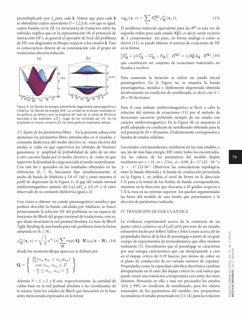
79

RE

VIS

TA C

UB

AN

A D

E F

ÍSIC

A,

Vol. 3

1,

No.

2 (

20

14

)AR

TÍCU

LOS

ORIG

INAL

ESE

d. E

. A

ltsh

uler

premultiplicarlo por Ik para cada k. Nótese que para cada k se obtendrán cuatro autovalores (l = 1,2,3,4), o lo que es igual, cuatro bandas en la ZB. La invariancia de traslación sobre las subredes implica que en la representación (8) el potencial de interacción HF y en general el operador de Fock del problema de HF, son diagonales en bloque respecto a los estados k. Esto es consecuencia directa de su conmutación con el grupo de traslaciones discreta reducido. (a) (b)

Figura 4: (a) Banda de energía doblemente degenerada paramagnética y metálica. (b) Banda de energía AFA. La unidad de la escala mostrada en los gráficos se define como la longitud del lado de la celda de Brillouin asociada a las subredes: , luego de ser divididas por 20. Se ha empleado el mismo convenio en los otros gráficos mostrados debajo.

3.1 Ajuste de los parámetros libres En la presente subsección ajustamos los parámetros libres introducidos en el modelo, є: constante dieléctrica del medio efectivo; m : masa efectiva del medio; ã: radio en que superviven los orbitales de Wannier gaussianos; γ : amplitud de probabilidad de salto de un sitio a otro cercano fijada por el medio efectivo y b : radio en que supervive la densidad de carga asociada al medio neutralizante. Con este fin y apoyados en los resultados obtenidos en las referencias [6, 7, 8], buscamos fijar simultáneamente: el ancho de banda de Matheiss a 3,8 eV (tal y como muestra el perfil de dispersión de la Figura 1), el gap del estado normal antiferromagnético aislante del La2CuO4 a 2,0 eV y el valor observado de su constante dieléctrica igual a 21.

Con vistas a obtener un estado paramagnético metálico que pudiera describir la banda calculada por Mathiess, se buscó primeramente la solución HF del porblema en un espacio de funciones de Bloch del grupo maximal de traslaciones, esto es, que dejan invariante la red puntual absoluta. La base de Bloch Tight-Binding de una banda para este problema tiene la forma adoptada en [6, 7, 8] ,

ϕσz

Q (x, s) =

√1

Nuσz(s)

∑R

exp(iQ ·R)ϕ0(x−R),

(14)

donde los momenta Q que aparecen se definen por

Q =

2πLp

(nx1ex1 + nx2ex2)

con nx1 , nx2 ∈ Z

−L2 ≤ nx1 , nx2 < L

2

.

Además N = L × L y R son, respectivamente, la cantidad de celdas base en la red puntual absoluta y las coordenadas de la misma. Sean los estados de Bloch que buscamos en la base antes mencionada expresados en la forma:

φQ,l(x, s) =∑σz

BQ,lσz

ϕσz

Q (x, s).

(15)

El problema matricial equivalente para las BQ,l es esta vez de segundo orden para cada estado (Q,l), es decir, serán vectores de 2 componentes. Así pues, en forma análoga a como se derivó (11), se puede obtener el sistema de ecuaciones de HF en la forma:[E0

Q + χ(GCQ −Gi

Q − FQ)]·BQ,l = εl(Q)IQ ·BQ,l, (16)

que constituyen un conjunto de ecuaciones matriciales no lineales a resolver.

Para comenzar la iteración se utilizó un estado inicial paramagnético. En la Figura 4a, se muestra la banda paramagnética, metálica y doblemente degenerada obtenida iterativamente en condición de semillenado, es decir con N = 20 × 20 electrones.

Para el caso aislante antiferromagnético se llevó a cabo la solución del sistema de ecuaciones (11) por el método de iteraciones sucesivas partiendo siempre de un estado con carácter antiferromagnético. En la Figura 4b, se muestran el perfil adoptado en condición de semillenado obtenido para la red puntual de 20 × 20 puntos. Evidentemente corresponden a bandas de estados aislantes.

Los estados correspondientes, resultaron ser los más estables, o sea, los de más baja energía (HF) entre todos los encontrados. Así los valores de los parámetros del modelo fijados resultaron ser: є = 21, m = 2.5me, ã = 0.09, b = 17.125 · 10−3 y γ = −17.125·10−3. Obsérvese las coincidencias topológicas entre la banda obtenida y la banda de conducción presentada en la Figura 1, en ambas el nivel de Fermi en la dirección Γ-X pasa a la mitad de los bordes de banda correspondiente, mientras en la dirección que descansa a 45 grados respecto a Γ-X la roza en su extremo superior. Así quedan argumentadas las bases del modelo de una banda que presentamos y la elección de parámetros realizada.

IV. TRANSICIÓN DE FASE CUÁNTICA

La evidencia experimental acerca de la existencia de un punto crítico cuántico en el La2CuO4 proviene de un estudio exhaustivo hecho por Jeffery Tallon y John Loram acerca de las propiedades físicas de la fase de pseudogap a partir de un gran cuerpo de experimentos de termodinámica que ellos mismos realizaron [5]. Encontraron que el pseudogap se caracteriza por una energía característica que cae abruptamente a cero en el dopaje crítico de 0.19 huecos, por átomo de cobre en el plano de conducción de un variado número de cupratos. Propiedades como la capacidad calorífica electrónica cambian abruptamente en el valor del dopaje crítico, lo cual indica que puede existir una transición a temperatura cero entre dos fases distintas. Pensando en ello, y una vez precisados los estados AFA y PPG en condición de semillenado, para los valores mejorados de los parámetros del modelo, nos propusimos reconsiderar el estudio presentado en [13, 14], para la evolución

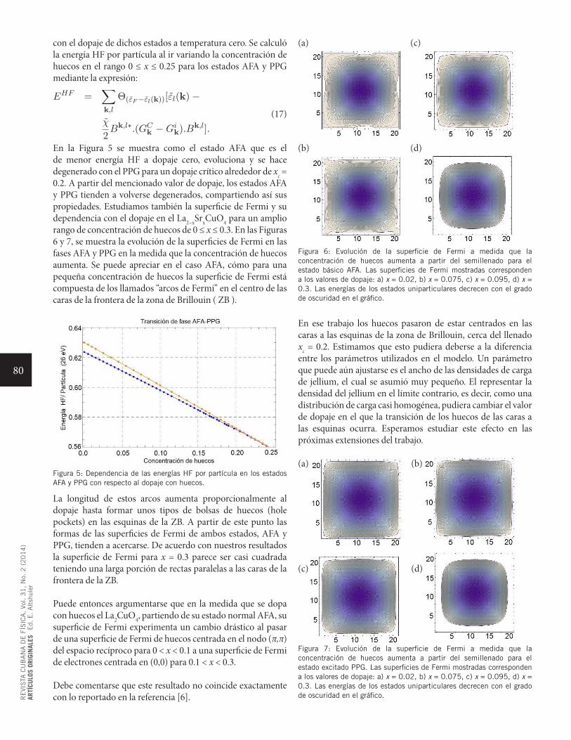
80

RE

VIS

TA C

UB

AN

A D

E F

ÍSIC

A,

Vol. 3

1,

No.

2 (

20

14

)AR

TÍCU

LOS

ORIG

INAL

ESE

d. E

. A

ltsh

uler

con el dopaje de dichos estados a temperatura cero. Se calculó la energía HF por partícula al ir variando la concentración de huecos en el rango 0 ≤ x ≤ 0.25 para los estados AFA y PPG mediante la expresión:

EHF =∑k,l

Θ(εF−εl(k))[εl(k)−

χ

2Bk,l∗.(GC

k −Gik).B

k,l].

(17)

En la Figura 5 se muestra como el estado AFA que es el de menor energía HF a dopaje cero, evoluciona y se hace degenerado con el PPG para un dopaje crítico alrededor de xc = 0.2. A partir del mencionado valor de dopaje, los estados AFA y PPG tienden a volverse degenerados, compartiendo así sus propiedades. Estudiamos también la superficie de Fermi y su dependencia con el dopaje en el La2−xSrxCuO4 para un amplio rango de concentración de huecos de 0 ≤ x ≤ 0.3. En las Figuras 6 y 7, se muestra la evolución de la superficies de Fermi en las fases AFA y PPG en la medida que la concentración de huecos aumenta. Se puede apreciar en el caso AFA, cómo para una pequeña concentración de huecos la superficie de Fermi está compuesta de los llamados “arcos de Fermi” en el centro de las caras de la frontera de la zona de Brillouin ( ZB ).

Figura 5: Dependencia de las energías HF por partícula en los estados AFA y PPG con respecto al dopaje con huecos.

La longitud de estos arcos aumenta proporcionalmente al dopaje hasta formar unos tipos de bolsas de huecos (hole pockets) en las esquinas de la ZB. A partir de este punto las formas de las superficies de Fermi de ambos estados, AFA y PPG, tienden a acercarse. De acuerdo con nuestros resultados la superficie de Fermi para x = 0.3 parece ser casi cuadrada teniendo una larga porción de rectas paralelas a las caras de la frontera de la ZB.

Puede entonces argumentarse que en la medida que se dopa con huecos el La2CuO4, partiendo de su estado normal AFA, su superficie de Fermi experimenta un cambio drástico al pasar de una superficie de Fermi de huecos centrada en el nodo (π,π) del espacio recíproco para 0 < x < 0.1 a una superficie de Fermi de electrones centrada en (0,0) para 0.1 < x < 0.3.

Debe comentarse que este resultado no coincide exactamente con lo reportado en la referencia [6].

Figura 6: Evolución de la superficie de Fermi a medida que la concentración de huecos aumenta a partir del semillenado para el estado básico AFA. Las superficies de Fermi mostradas corresponden a los valores de dopaje: a) x = 0.02, b) x = 0.075, c) x = 0.095, d) x = 0.3. Las energías de los estados uniparticulares decrecen con el grado de oscuridad en el gráfico.

En ese trabajo los huecos pasaron de estar centrados en las caras a las esquinas de la zona de Brillouin, cerca del llenado xc = 0.2. Estimamos que esto pudiera deberse a la diferencia entre los parámetros utilizados en el modelo. Un parámetro que puede aún ajustarse es el ancho de las densidades de carga de jellium, el cual se asumió muy pequeño. El representar la densidad del jellium en el límite contrario, es decir, como una distribución de carga casi homogénea, pudiera cambiar el valor de dopaje en el que la transición de los huecos de las caras a las esquinas ocurra. Esperamos estudiar este efecto en las próximas extensiones del trabajo.

Figura 7: Evolución de la superficie de Fermi a medida que la concentración de huecos aumenta a partir del semillenado para el estado excitado PPG. Las superficies de Fermi mostradas corresponden a los valores de dopaje: a) x = 0.02, b) x = 0.075, c) x = 0.095, d) x = 0.3. Las energías de los estados uniparticulares decrecen con el grado de oscuridad en el gráfico.

(a) (c)

(b) (d)

(a) (b)

(c) (d)

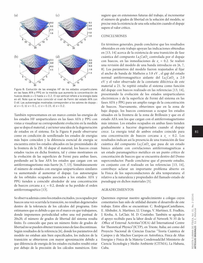
81

RE

VIS

TA C

UB

AN

A D

E F

ÍSIC

A,

Vol. 3

1,

No.

2 (

20

14

)AR

TÍCU

LOS

ORIG

INAL

ESE

d. E

. A

ltsh

uler

Figura 8: Evolución de las energías HF de los estados uniparticulares en las fases AFA y PPG en la medida que aumenta la concentración de huecos desde x = 0 hasta x = 0.2. El eje vertical refiere a la energía dada en eV. Note que se hace coincidir el nivel de Fermi del estado AFA con 0 eV. Las autoenergías mostradas corresponden a los valores de dopaje : a) x = 0, b) x = 0.1, c) x = 0.15, d) x = 0.2.

También representamos en un marco común las energías de los estados HF uniparticulares en las fases AFA y PPG con vistas a visualizar su correspondiente evolución en la medida que se dopa el material, y así tener una idea de la degeneración de estados en el sistema. En la Figura 8 puede observarse como en condición de semillenado los estados de energías más bajos coinciden y la diferencia esencial de energía se encuentra entre los estados ubicados en las proximidades de la frontera de la ZB. Al dopar el material, los huecos crean estados vacíos en dicha frontera, tal y cómo mostramos en la evolución de las superficies de Fermi para ambas fases, perdiendo así la fase AFA los estados que cargan con un antiferromagnetismo más fuerte [6, 7, 13]. Simultáneamente el número de estados con energías uniparticulares similares va aumentando al aumentar el dopaje. Las autoenergías de los orbitales ocupados asociados a los estados AFA y PPG tienden a coincidir alrededor de una concentración de huecos cercana a xc = 0.2, donde se ha perdido el orden antiferromagnético [13].

Se observa además como los estados excitados, ya ocupados por huecos una vez ocurrida la transición, no resultan degenerados dentro de la tolerancia de los cálculos del programa. Esto estimamos que es debido a que en el marco en que trabajamos, donde imponemos periodicidad sobre una red puntual de 20x20, el número de grados de libertad del sistema resulta finito. Es conocido que para un número finito de grados de libertad no se pueden obtener transiciones de fase discontinuas. Según resultados de la referencia [6], donde los parámetros del modelo no estaban aún bien especificados, los indicios de la transición se obtuvieron con mayor aproximación debido a que diferencia de energía de los estados excitados resultó estar por debajo de la precisión de los cálculos numéricos. Esto

sugiere que en extensiones futuras del trabajo, al incrementar el número de grados de libertad en la solución del modelo, se precise más la existencia de una sola solución cuando el dopaje supere el valor crítico.

CONCLUSIONES

En términos generales, puede concluirse que los resultados obtenidos en este trabajo apoyan las indicaciones obtendias en [13, 14] acerca de la existencia de una transición de fase cuántica del compuesto La2CuO4 controlada por el dopaje con huecos, en las inmediaciones de xc = 0.2. Se realizó una revisión del modelo de una banda introducio en [6, 7, 8]. Los parámetros del modelo fueron reajustados al fijar el ancho de banda de Matheiss a 3.8 eV , el gap del estado normal antiferromagnético aislante del La2CuO4 a 2.0 eV y el valor observado de la constante diléctrica de este material a 21. Se repitió estudio el sistema como función del dopaje con huecos realizado en las referencias [13, 14], presentando la evolución de los estados uniparticulares electrónicos y de la superficie de Fermi del sistema en las fases AFA y PPG para un amplio rango de la concentración de huecos. Nuevamente, obtuvimos que en la zona de bajo dopaje, los huecos comienzan a ocupar los estados situados en la frontera de la zona de Brillouin y que en el estado AFA son los que cargan con el antiferromagnetismo más intenso. Los estados ocupados en ambas fases tienden gradualmente a hacerse degenerados cuando el dopaje crece. La energía total de ambos estados coincide para una concentración de huecos cercana a xc = 0.2. Los resultados indican así la presencia de una transición de fase cuántica del compuesto La2CuO4 que pasa de un estado básico aislante con correlaciones antiferromagnéticas a un estado paramagnético metálico en un punto crítico de concentación de huecos que se encuentra dentro del Domo superconductor. Puede concluirse que el presente estudio, en conjunto con el realizado en las referencias [13, 14], contribuye aclarar un importante problema abierto en la Física de los superconductores de alta temperatura: el relativo a la naturaleza y propiedades del llamado estado de pseudogap en dichos materiales [5].

AGRADECIMIENTOS

Queremos expresar nuestro agradecimiento a colegas cuyos comentarios han sido de utilidad durante el desarrollo de este trabajo. Entre ellos se encuentran: C. RodríguezCastellanos, E. Altshuler, A. Martínez, Ll. Uranga, V. Martínez, E. Fradkin, J. Kroha, A. LeClair, M. D. Coutinho. También se agradece el apoyo recibido para la labor desde el Network N-35 de la .Office of External Activities”(OEA) del Ïnternational Centre for Theoretical Physics”(ICTP), en Trieste, Italia; así como del Proyecto Nacional de Ciencias Exactas “Teoría Cuántica de Campos y de Muchos Cuerpos en Astrofísica, Física de Altas Energías y Física de la Materia Condensada”del Ministerio de Ciencia Tecnología y Medio Ambiente (CITMA), La Habana, Cuba.

(a) (c)

(d)(b)

82

RE

VIS

TA C

UB

AN

A D

E F

ÍSIC

A,

Vol. 3

1,

No.

2 (

20

14

)AR

TÍCU

LOS

ORIG

INAL

ESE

d. E

. A

ltsh

uler

[1] J. G. Bednorz y K. A. Müller, Zeitschriftfür, Z. Phys. B: Condens. Matter 64, 189 (1986).[2] G. Deutscher, Rev. Mod. Phys. 77, 109 (2005).[3] S. A. Kivelson, E. Fradkin, Va. Oganesyan, I. Bindloss, J. Tranquada, A. Kapitulnik y C. Howald, Rev. Mod. Phys. 75, 1201 (2003).[4] J. M. Tranquada, Treatise of High Temperature Superconductivity, J. R. Schrieffer and J. Brooks, eds., (Springer-Verlag, 2007) pp. 257– 298.[5] J. L. Tallon y J. W. Loram, Physica C 349, 53 (2001).[6] A. Cabo-Bizet, “Una aproximación Hartree Fock al antiferromagnetismo del La2CuO4”, Tesis de Diploma, Facultad de Física, Universidad de La Habana, 2008.[7] A. Cabo-Bizet y A. Cabo Montes de Oca, Phys. Lett. A 373, 1865 (2009).[8] A. Cabo-Bizet y A. Cabo Montes de Oca, Symmetry 2, 388 (2010).[9] J. K. Perry, J. Tahir-Kheli and W.A. Goddard III, Phys. Rev.

B 63, 144510 (2001). [10] C. Y. Chen, R. J. Birgeneau, M. A. Kastner, N. W. Preyer and Tineke Thio, Phys. Rev B 43 , 392 (1991).[11] L. F. Matheiss, Phys. Rev. Lett. 58, 1028 (1987).[12] E. Fradkin, Field Theory of Condensed Matter Systems, (Addison-Wesley, New York, 1991). [13] V. M. Martínez, “Transición de fase cuántica dentro del domo superconductor”, Tesis de Diploma, Facultad de Física, Universidad de La Habana, 2012.[14] V. M. Martinez Alvarez, A. Cabo-Bizet and A. Cabo Montes de Oca, Int. J. Mod. Phys. B 28, 1450146 (2014).[15] P. A. M. Dirac, Proc. Cambridge Philos. Soc. 26, 376 (1930).[16] F. F. Balakirev, J. B. Betts, A. Migliori, I. Tsukada, Y. Ando y G. S. Boebinger, Phys. Rev. Lett. 102, 017004 (2009).[17] R. Daou, y col, Nat. Phys. 5, 31 (2009).[18] Y. Yanase, Physics Reports 387, 1 (2003).[19] W. E. Pickett, Rev. Mod. Phys. 61, 433 (1989).

83

RE

VIS

TA C

UB

AN

A D

E F

ÍSIC

A,

Vol. 3

1,

No.

2 (

20

14

)AR

TÍCU

LOS

ORIG

INAL

ESE

d. E

. A

ltsh

uler

ARTÍCULO ORIGINAL

ESTABILIDAD, OBSERVABILIDAD, CONTROLABILIDAD Y RESPUESTA A FRECUENCIAS DE UN CONMUTADOR OPTOELECTRÓNICO DE VO2, CONSIDERADO COMO UN DISPOSITIVO DE ENTRADA-SALIDA EN REPRESENTACIONES TF, SS Y ZPKSTABILITY, OBSERVABILITY, CONTROLABILITY AND FREQUENCY RESPONSE OF A VO2 OPTOELECTRONIC COMMUTER, ASSUMING IT AS AN INPUT-OUTPUT DEVICE IN THE TF, SS AND ZPK REPRESENTATIONS

L. Benavides

Facultad de Ingeniería Eléctrica, Instituto Superior Politécnico José Antonio Echeverría, Cuba, leonard@electrica.cujae.edu.cu

(Recibido 17/2/2014 ; Aceptado 6/11/2014)

Se analizan los conmutadores optoelectrónicos, basados en láminas delgadas de VO2, como dispositivos de entrada-salida (E/S) de respuesta múltiple a estímulos de tensión eléctrica, temperatura y energía de la radiación electromagnética incidente. Se utilizan las representaciones de estos dispositivos sobre la base de su función transferencial (TF), en el espacio de estado (SS) y en la representación de polos, ceros y ganancia (ZPK). A partir de ahí, se investiga la estabilidad, observabilidad, controlabilidad y respuesta a frecuencias de dichos sistemas, lo cual contribuye a una mejor comprensión del funcionamiento de los mismos y sus potenciales aplicaciones.

Optoelectronic switches based on VO2 thin films are analyzed as input-output devices (I/O) of multiple responses to stimuli of electric tension, temperature and energy of the incident electromagnetic radiation. The representations used are based on their transfer function (TF), in the space state (SS) and in the representation of poles, zeros and gain (ZPK). Starting from there, the stability, observability, controllability and frequency response of these systems are investigated, which contributes to a better understanding of the operation of these devices and their potential applications.

PACS: Optical computers, logic elements, interconnects, switches; neural networks 42.79.Ta, Optical properties of specific thin films 78.66.–w, Optoelectronic devices 85.60.–q

I. INTRODUCCIÓN

En los últimos años se han publicado numerosos trabajos científicos, tanto teóricos, como experimentales, referentes a las características físicas de los compuestos óxidos de vanadio y sus posibles aplicaciones en la optoelectrónica y la microelectrónica modernas [1-6]. Muchos de esos trabajos han centrado la atención en las características físicas de los conmutadores optoelectrónicos de respuesta múltiple, basados en láminas delgadas de VO2 [7-14]. Sin embargo, existen varios aspectos técnicos de estos dispositivos que no han sido aun suficientemente estudiados y que pudieran brindar más información para comprender mejor sus posibles aplicaciones. Por esas razones, en este trabajo se analizan los conmutadores optoelectrónicos, basados en láminas delgadas de VO2, como dispositivos de entrada-salida (E/S) de respuesta múltiple a estímulos de tensión eléctrica, temperatura y energía de la radiación electromagnética incidente. Se utilizan las representaciones

de estos dispositivos en base a su función transferencial (TF), en el espacio de estado (SS) y en la representación de polos, ceros y ganancia (ZPK) y, a partir de ahí, se investiga la estabilidad, observabilidad, controlabilidad y respuesta a frecuencias de dichos sistemas, lo cual contribuye a una mejor comprensión del funcionamiento de los mismos y sus potenciales aplicaciones prácticas.

II. ANÁLISIS DEL SISTEMA I-V

Para nuestro análisis se consideraron láminas delgadas de VO2, con orientación (100), depositadas epitaxialmente sobre un sustrato de zafiro cortado-R (Al2O3) [15]. El dispositivo de referencia fue considerado como un sistema de entrada-salida, lineal e invariante-temporal, en el cual la entrada está constituida por una secuencia de 25 señales de tensión directa y la salida como una secuencia de 25 intensidades de corriente. A este sistema lo denominaremos I-V y constituye un sistema de simple entrada-simple salida (SISO)

Rev. Cub. Fis. 31, 83 (2014)

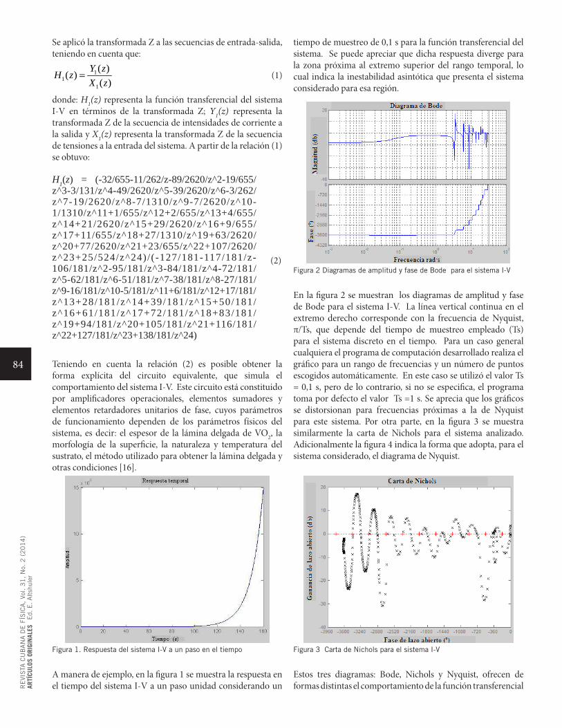
84

RE

VIS

TA C

UB

AN

A D

E F

ÍSIC

A,

Vol. 3

1,

No.

2 (

20

14

)AR

TÍCU

LOS

ORIG

INAL

ESE

d. E

. A

ltsh

uler

Se aplicó la transformada Z a las secuencias de entrada-salida, teniendo en cuenta que:

11

1

( )( )( )

Y zH zX z

=

(1)

donde: H1(z) representa la función transferencial del sistema I-V en términos de la transformada Z; Y1(z) representa la transformada Z de la secuencia de intensidades de corriente a la salida y X1(z) representa la transformada Z de la secuencia de tensiones a la entrada del sistema. A partir de la relación (1) se obtuvo:

H1(z) = (-32/655-11/262/z-89/2620/z^2-19/655/z^3-3/131/z^4-49/2620/z^5-39/2620/z^6-3/262/z^7-19/2620/z^8-7/1310/z^9-7/2620/z^10-1/1310/z^11+1/655/z^12+2/655/z^13+4/655/z^14+21/2620/z^15+29/2620/z^16+9/655/z^17+11/655/z^18+27/1310/z^19+63/2620/z^20+77/2620/z^21+23/655/z^22+107/2620/z^23+25/524/z^24)/(-127/181-117/181/z-106/181/z^2-95/181/z^3-84/181/z^4-72/181/z^5-62/181/z^6-51/181/z^7-38/181/z^8-27/181/z^9-16/181/z^10-5/181/z^11+6/181/z^12+17/181/z^13+28/181/z^14+39/181/z^15+50/181/z^16+61/181/z^17+72/181/z^18+83/181/z^19+94/181/z^20+105/181/z^21+116/181/z^22+127/181/z^23+138/181/z^24)

Teniendo en cuenta la relación (2) es posible obtener la forma explícita del circuito equivalente, que simula el comportamiento del sistema I-V. Este circuito está constituido por amplificadores operacionales, elementos sumadores y elementos retardadores unitarios de fase, cuyos parámetros de funcionamiento dependen de los parámetros físicos del sistema, es decir: el espesor de la lámina delgada de VO2, la morfología de la superficie, la naturaleza y temperatura del sustrato, el método utilizado para obtener la lámina delgada y otras condiciones [16].

Figura 1. Respuesta del sistema I-V a un paso en el tiempo

A manera de ejemplo, en la figura 1 se muestra la respuesta en el tiempo del sistema I-V a un paso unidad considerando un

(2)

tiempo de muestreo de 0,1 s para la función transferencial del sistema. Se puede apreciar que dicha respuesta diverge para la zona próxima al extremo superior del rango temporal, lo cual indica la inestabilidad asintótica que presenta el sistema considerado para esa región.

Figura 2 Diagramas de amplitud y fase de Bode para el sistema I-V

En la figura 2 se muestran los diagramas de amplitud y fase de Bode para el sistema I-V. La línea vertical continua en el extremo derecho corresponde con la frecuencia de Nyquist, π/Ts, que depende del tiempo de muestreo empleado (Ts) para el sistema discreto en el tiempo. Para un caso general cualquiera el programa de computación desarrollado realiza el gráfico para un rango de frecuencias y un número de puntos escogidos automáticamente. En este caso se utilizó el valor Ts = 0,1 s, pero de lo contrario, si no se especifica, el programa toma por defecto el valor Ts =1 s. Se aprecia que los gráficos se distorsionan para frecuencias próximas a la de Nyquist para este sistema. Por otra parte, en la figura 3 se muestra similarmente la carta de Nichols para el sistema analizado. Adicionalmente la figura 4 indica la forma que adopta, para el sistema considerado, el diagrama de Nyquist.

Figura 3 Carta de Nichols para el sistema I-V

Estos tres diagramas: Bode, Nichols y Nyquist, ofrecen de formas distintas el comportamiento de la función transferencial

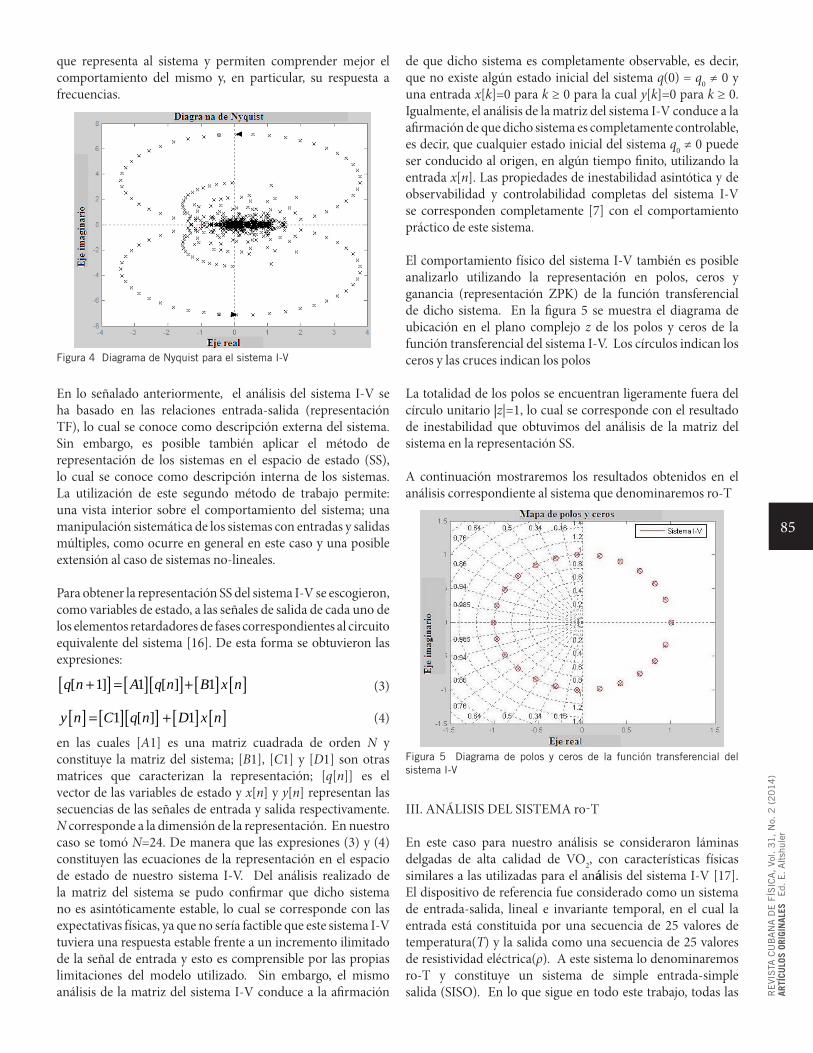
85

RE

VIS

TA C

UB

AN

A D

E F

ÍSIC

A,

Vol. 3

1,

No.

2 (

20

14

)AR

TÍCU

LOS

ORIG

INAL

ESE

d. E

. A

ltsh

uler

que representa al sistema y permiten comprender mejor el comportamiento del mismo y, en particular, su respuesta a frecuencias.

Figura 4 Diagrama de Nyquist para el sistema I-V

En lo señalado anteriormente, el análisis del sistema I-V se ha basado en las relaciones entrada-salida (representación TF), lo cual se conoce como descripción externa del sistema. Sin embargo, es posible también aplicar el método de representación de los sistemas en el espacio de estado (SS), lo cual se conoce como descripción interna de los sistemas. La utilización de este segundo método de trabajo permite: una vista interior sobre el comportamiento del sistema; una manipulación sistemática de los sistemas con entradas y salidas múltiples, como ocurre en general en este caso y una posible extensión al caso de sistemas no-lineales.

Para obtener la representación SS del sistema I-V se escogieron, como variables de estado, a las señales de salida de cada uno de los elementos retardadores de fases correspondientes al circuito equivalente del sistema [16]. De esta forma se obtuvieron las expresiones:

[ ] [ ][ ] [ ] [ ][ 1] 1 [ ] 1q n A q n B x n+ = + (3)

[ ] [ ][ ] [ ] [ ]1 [ ] 1y n C q n D x n= + (4)

en las cuales [A1] es una matriz cuadrada de orden N y constituye la matriz del sistema; [B1], [C1] y [D1] son otras matrices que caracterizan la representación; [q[n]] es el vector de las variables de estado y x[n] y y[n] representan las secuencias de las señales de entrada y salida respectivamente. N corresponde a la dimensión de la representación. En nuestro caso se tomó N=24. De manera que las expresiones (3) y (4) constituyen las ecuaciones de la representación en el espacio de estado de nuestro sistema I-V. Del análisis realizado de la matriz del sistema se pudo confirmar que dicho sistema no es asintóticamente estable, lo cual se corresponde con las expectativas físicas, ya que no sería factible que este sistema I-V tuviera una respuesta estable frente a un incremento ilimitado de la señal de entrada y esto es comprensible por las propias limitaciones del modelo utilizado. Sin embargo, el mismo análisis de la matriz del sistema I-V conduce a la afirmación

de que dicho sistema es completamente observable, es decir, que no existe algún estado inicial del sistema q(0) = q0 ≠ 0 y una entrada x[k]=0 para k ≥ 0 para la cual y[k]=0 para k ≥ 0. Igualmente, el análisis de la matriz del sistema I-V conduce a la afirmación de que dicho sistema es completamente controlable, es decir, que cualquier estado inicial del sistema q0 ≠ 0 puede ser conducido al origen, en algún tiempo finito, utilizando la entrada x[n]. Las propiedades de inestabilidad asintótica y de observabilidad y controlabilidad completas del sistema I-V se corresponden completamente [7] con el comportamiento práctico de este sistema.

El comportamiento físico del sistema I-V también es posible analizarlo utilizando la representación en polos, ceros y ganancia (representación ZPK) de la función transferencial de dicho sistema. En la figura 5 se muestra el diagrama de ubicación en el plano complejo z de los polos y ceros de la función transferencial del sistema I-V. Los círculos indican los ceros y las cruces indican los polos

La totalidad de los polos se encuentran ligeramente fuera del círculo unitario |z|=1, lo cual se corresponde con el resultado de inestabilidad que obtuvimos del análisis de la matriz del sistema en la representación SS.

A continuación mostraremos los resultados obtenidos en el análisis correspondiente al sistema que denominaremos ro-T

Figura 5 Diagrama de polos y ceros de la función transferencial del sistema I-V

III. ANÁLISIS DEL SISTEMA ro-T

En este caso para nuestro análisis se consideraron láminas delgadas de alta calidad de VO2, con características físicas similares a las utilizadas para el análisis del sistema I-V [17]. El dispositivo de referencia fue considerado como un sistema de entrada-salida, lineal e invariante temporal, en el cual la entrada está constituida por una secuencia de 25 valores de temperatura(T) y la salida como una secuencia de 25 valores de resistividad eléctrica(ρ). A este sistema lo denominaremos ro-T y constituye un sistema de simple entrada-simple salida (SISO). En lo que sigue en todo este trabajo, todas las

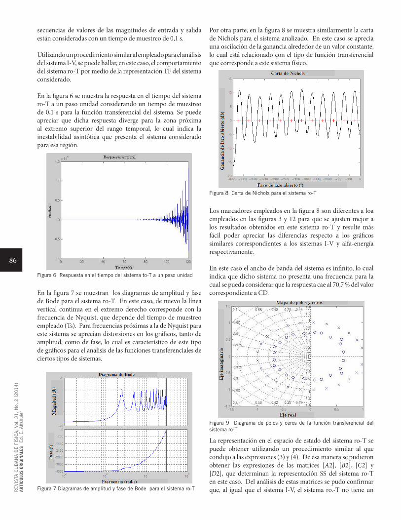
86

RE

VIS

TA C

UB

AN

A D

E F

ÍSIC

A,

Vol. 3

1,

No.

2 (

20

14

)AR

TÍCU

LOS

ORIG

INAL

ESE

d. E

. A

ltsh

uler

secuencias de valores de las magnitudes de entrada y salida están consideradas con un tiempo de muestreo de 0,1 s.

Utilizando un procedimiento similar al empleado para el análisis del sistema I-V, se puede hallar, en este caso, el comportamiento del sistema ro-T por medio de la representación TF del sistema considerado.

En la figura 6 se muestra la respuesta en el tiempo del sistema ro-T a un paso unidad considerando un tiempo de muestreo de 0,1 s para la función transferencial del sistema. Se puede apreciar que dicha respuesta diverge para la zona próxima al extremo superior del rango temporal, lo cual indica la inestabilidad asintótica que presenta el sistema considerado para esa región.

Figura 6 Respuesta en el tiempo del sistema to-T a un paso unidad

En la figura 7 se muestran los diagramas de amplitud y fase de Bode para el sistema ro-T. En este caso, de nuevo la línea vertical continua en el extremo derecho corresponde con la frecuencia de Nyquist, que depende del tiempo de muestreo empleado (Ts). Para frecuencias próximas a la de Nyquist para este sistema se aprecian distorsiones en los gráficos, tanto de amplitud, como de fase, lo cual es característico de este tipo de gráficos para el análisis de las funciones transferenciales de ciertos tipos de sistemas.

Figura 7 Diagramas de amplitud y fase de Bode para el sistema ro-T

Por otra parte, en la figura 8 se muestra similarmente la carta de Nichols para el sistema analizado. En este caso se aprecia una oscilación de la ganancia alrededor de un valor constante, lo cual está relacionado con el tipo de función transferencial que corresponde a este sistema físico.

Figura 8 Carta de Nichols para el sistema ro-T

Los marcadores empleados en la figura 8 son diferentes a loa empleados en las figuras 3 y 12 para que se ajusten mejor a los resultados obtenidos en este sistema ro-T y resulte más fácil poder apreciar las diferencias respecto a los gráficos similares correspondientes a los sistemas I-V y alfa-energía respectivamente.

En este caso el ancho de banda del sistema es infinito, lo cual indica que dicho sistema no presenta una frecuencia para la cual se pueda considerar que la respuesta cae al 70,7 % del valor correspondiente a CD.

Figura 9 Diagrama de polos y ceros de la función transferencial del sistema ro-T

La representación en el espacio de estado del sistema ro-T se puede obtener utilizando un procedimiento similar al que condujo a las expresiones (3) y (4). De esa manera se pudieron obtener las expresiones de las matrices [A2], [B2], [C2] y [D2], que determinan la representación SS del sistema ro-T en este caso. Del análisis de estas matrices se pudo confirmar que, al igual que el sistema I-V, el sistema ro.-T no tiene un

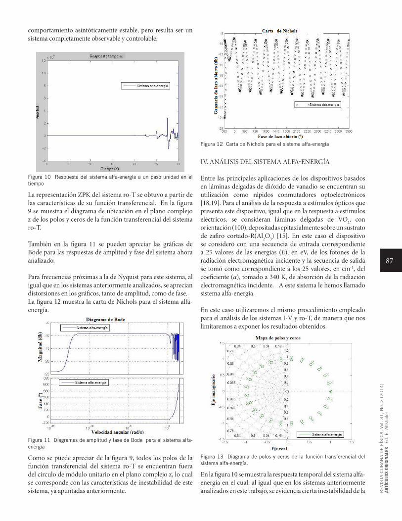
87

RE

VIS

TA C

UB

AN

A D

E F

ÍSIC

A,

Vol. 3

1,

No.

2 (

20

14

)AR

TÍCU

LOS

ORIG

INAL

ESE

d. E

. A

ltsh

uler

comportamiento asintóticamente estable, pero resulta ser un sistema completamente observable y controlable.

Figura 10 Respuesta del sistema alfa-energía a un paso unidad en el tiempo

La representación ZPK del sistema ro-T se obtuvo a partir de las características de su función transferencial. En la figura 9 se muestra el diagrama de ubicación en el plano complejo z de los polos y ceros de la función transferencial del sistema ro-T.

También en la figura 11 se pueden apreciar las gráficas de Bode para las respuestas de amplitud y fase del sistema ahora analizado.

Para frecuencias próximas a la de Nyquist para este sistema, al igual que en los sistemas anteriormente analizados, se aprecian distorsiones en los gráficos, tanto de amplitud, como de fase.La figura 12 muestra la carta de Nichols para el sistema alfa-energía.

Figura 11 Diagramas de amplitud y fase de Bode para el sistema alfa-energía

Como se puede apreciar de la figura 9, todos los polos de la función transferencial del sistema ro-T se encuentran fuera del círculo de módulo unitario en el plano complejo z, lo cual se corresponde con las características de inestabilidad de este sistema, ya apuntadas anteriormente.

Figura 12 Carta de Nichols para el sistema alfa-energía

IV. ANÁLISIS DEL SISTEMA ALFA-ENERGÍA

Entre las principales aplicaciones de los dispositivos basados en láminas delgadas de dióxido de vanadio se encuentran su utilización como rápidos conmutadores optoelectrónicos [18,19]. Para el análisis de la respuesta a estímulos ópticos que presenta este dispositivo, igual que en la respuesta a estímulos eléctricos, se consideran láminas delgadas de VO2, con orientación (100), depositadas epitaxialmente sobre un sustrato de zafiro cortado-R(Al2O3) [15]. En este caso el dispositivo se consideró con una secuencia de entrada correspondiente a 25 valores de las energías (E), en eV, de los fotones de la radiación electromagnética incidente y la secuencia de salida se tomó como correspondiente a los 25 valores, en cm-1, del coeficiente (α), tomado a 340 K, de absorción de la radiación electromagnética incidente. A este sistema le hemos llamado sistema alfa-energía.

En este caso utilizaremos el mismo procedimiento empleado para el análisis de los sistemas I-V y ro-T, de manera que nos limitaremos a exponer los resultados obtenidos.

Figura 13 Diagrama de polos y ceros de la función transferencial del sistema alfa-energía.

En la figura 10 se muestra la respuesta temporal del sistema alfa-energía en el cual, al igual que en los sistemas anteriormente analizados en este trabajo, se evidencia cierta inestabilidad de la

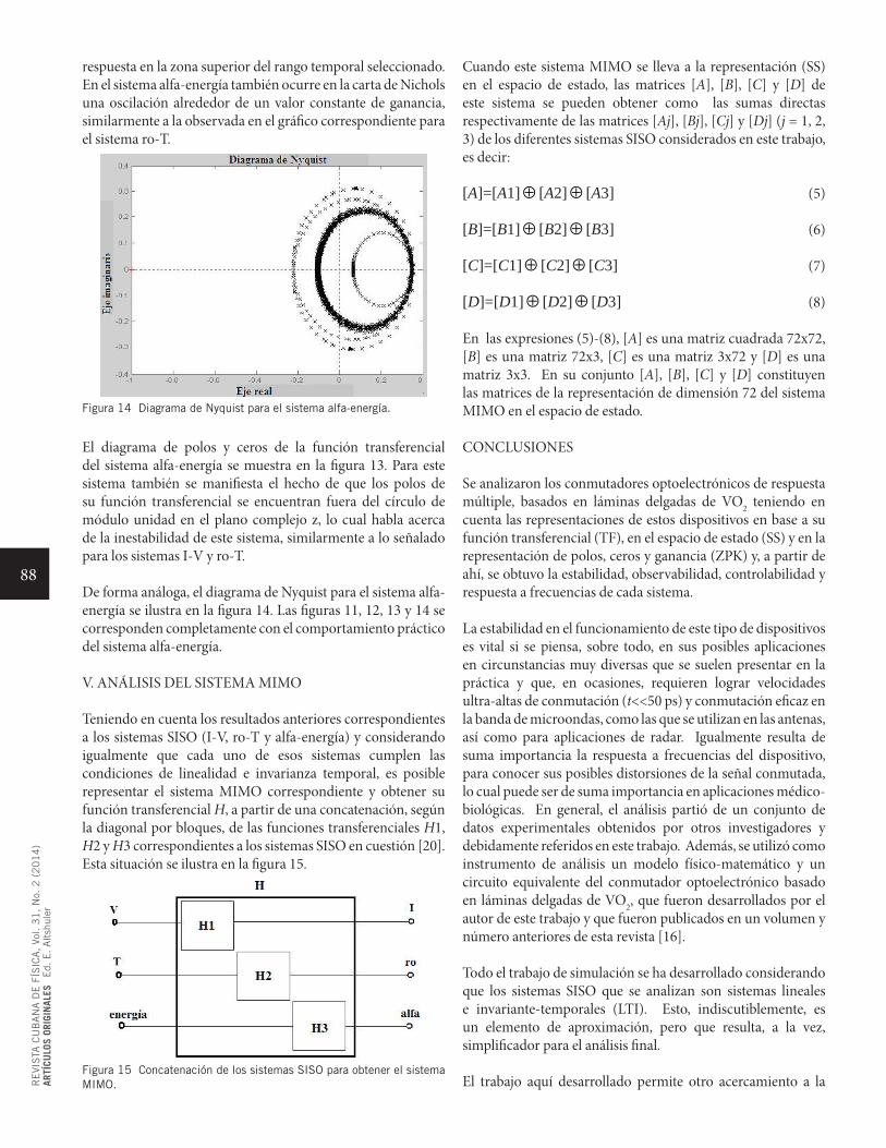
88

RE

VIS

TA C

UB

AN

A D

E F

ÍSIC

A,

Vol. 3

1,

No.

2 (

20

14

)AR

TÍCU

LOS

ORIG

INAL

ESE

d. E

. A

ltsh

uler

respuesta en la zona superior del rango temporal seleccionado.En el sistema alfa-energía también ocurre en la carta de Nichols una oscilación alrededor de un valor constante de ganancia, similarmente a la observada en el gráfico correspondiente para el sistema ro-T.

Figura 14 Diagrama de Nyquist para el sistema alfa-energía.

El diagrama de polos y ceros de la función transferencial del sistema alfa-energía se muestra en la figura 13. Para este sistema también se manifiesta el hecho de que los polos de su función transferencial se encuentran fuera del círculo de módulo unidad en el plano complejo z, lo cual habla acerca de la inestabilidad de este sistema, similarmente a lo señalado para los sistemas I-V y ro-T.

De forma análoga, el diagrama de Nyquist para el sistema alfa-energía se ilustra en la figura 14. Las figuras 11, 12, 13 y 14 se corresponden completamente con el comportamiento práctico del sistema alfa-energía.

V. ANÁLISIS DEL SISTEMA MIMO

Teniendo en cuenta los resultados anteriores correspondientes a los sistemas SISO (I-V, ro-T y alfa-energía) y considerando igualmente que cada uno de esos sistemas cumplen las condiciones de linealidad e invarianza temporal, es posible representar el sistema MIMO correspondiente y obtener su función transferencial H, a partir de una concatenación, según la diagonal por bloques, de las funciones transferenciales H1, H2 y H3 correspondientes a los sistemas SISO en cuestión [20]. Esta situación se ilustra en la figura 15.

Figura 15 Concatenación de los sistemas SISO para obtener el sistema MIMO.

Cuando este sistema MIMO se lleva a la representación (SS) en el espacio de estado, las matrices [A], [B], [C] y [D] de este sistema se pueden obtener como las sumas directas respectivamente de las matrices [Aj], [Bj], [Cj] y [Dj] (j = 1, 2, 3) de los diferentes sistemas SISO considerados en este trabajo, es decir:

[A]=[A1] ⊕ [A2] ⊕ [A3] (5)

[B]=[B1] ⊕ [B2] ⊕ [B3] (6)

[C]=[C1] ⊕ [C2] ⊕ [C3] (7)

[D]=[D1] ⊕ [D2] ⊕ [D3] (8)

En las expresiones (5)-(8), [A] es una matriz cuadrada 72x72, [B] es una matriz 72x3, [C] es una matriz 3x72 y [D] es una matriz 3x3. En su conjunto [A], [B], [C] y [D] constituyen las matrices de la representación de dimensión 72 del sistema MIMO en el espacio de estado.

CONCLUSIONES

Se analizaron los conmutadores optoelectrónicos de respuesta múltiple, basados en láminas delgadas de VO2 teniendo en cuenta las representaciones de estos dispositivos en base a su función transferencial (TF), en el espacio de estado (SS) y en la representación de polos, ceros y ganancia (ZPK) y, a partir de ahí, se obtuvo la estabilidad, observabilidad, controlabilidad y respuesta a frecuencias de cada sistema.

La estabilidad en el funcionamiento de este tipo de dispositivos es vital si se piensa, sobre todo, en sus posibles aplicaciones en circunstancias muy diversas que se suelen presentar en la práctica y que, en ocasiones, requieren lograr velocidades ultra-altas de conmutación (t<<50 ps) y conmutación eficaz en la banda de microondas, como las que se utilizan en las antenas, así como para aplicaciones de radar. Igualmente resulta de suma importancia la respuesta a frecuencias del dispositivo, para conocer sus posibles distorsiones de la señal conmutada, lo cual puede ser de suma importancia en aplicaciones médico-biológicas. En general, el análisis partió de un conjunto de datos experimentales obtenidos por otros investigadores y debidamente referidos en este trabajo. Además, se utilizó como instrumento de análisis un modelo físico-matemático y un circuito equivalente del conmutador optoelectrónico basado en láminas delgadas de VO2, que fueron desarrollados por el autor de este trabajo y que fueron publicados en un volumen y número anteriores de esta revista [16].

Todo el trabajo de simulación se ha desarrollado considerando que los sistemas SISO que se analizan son sistemas lineales e invariante-temporales (LTI). Esto, indiscutiblemente, es un elemento de aproximación, pero que resulta, a la vez, simplificador para el análisis final.

El trabajo aquí desarrollado permite otro acercamiento a la

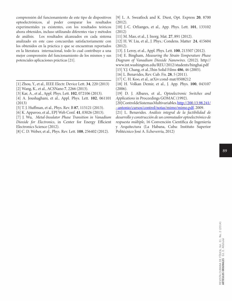
89

RE

VIS

TA C

UB

AN

A D

E F

ÍSIC

A,

Vol. 3

1,

No.

2 (

20

14

)AR

TÍCU

LOS

ORIG

INAL

ESE

d. E

. A

ltsh

uler

comprensión del funcionamiento de este tipo de dispositivos optoelectrónicos, al poder comparar los resultados experimentales ya existentes, con los resultados teóricos ahora obtenidos, incluso utilizando diferentes vías y métodos de análisis. Los resultados alcanzados en cada sistema analizado en este caso concuerdan satisfactoriamente con los obtenidos en la práctica y que se encuentran reportados en la literatura internacional, todo lo cual contribuye a una mejor comprensión del funcionamiento de los mismos y sus potenciales aplicaciones prácticas [21].

[1] Zhou, Y., et al., IEEE Electr. Device Lett. 34, 220 (2013)[2] Wang, K., et al., ACSNano 7, 2266 (2013).[3] Kar, A., et al., Appl. Phys. Lett. 102, 072106 (2013).[4] A. Joushaghani, et al., Appl. Phys. Lett. 102, 061101 (2013)[5] T. J. Huffman, et al., Phys. Rev. B 87, 115121 (2013).[6] K. Appavoo, et al., EPJ Web Conf. 41, 03026 (2013).[7] J. Wu, Metal-Insulator Phase Transition in Vanadium Dioxide for Electronics, in Center for Energy Efficient Electronics Science (2012). [8] C. D. Weber, et al., Phys. Rev. Lett. 108, 256402 (2012).

[9] L. A. Sweatlock and K. Diest, Opt. Express 20, 8700 (2012).[10] J.-C. Orlianges, et al., App. Phys. Lett. 101, 133102 (2012)[11] M. Mao, et al., J. Inorg. Mat. 27, 891 (2012).[12] H. W. Liu, et al., J. Phys.: Condens. Matter 24, 415604 (2012).[13]. J. Leroy, et al., Appl. Phys. Lett. 100, 213507 (2012).[14] E. Bingham, Measuring the Strain-Temperature Phase Diagram of Vanadium Dioxide Nanowires. (2012). http://www.int.washington.edu/REU/2012/students/binghai.pdf[15] Y.J. Chang, et al.,Thin Solid Films 486, 46 (2005).[16] L. Benavides, Rev. Cub. Fis. 28, 5 (2011).[17] C. H. Koo, et al., arXiv:cond-mat/0508212[18] H. Volkan Demir, et al., J. App. Phys. 100, 043107 (2006).[19] D. J. Albares, et al., Optoelectronic Switches and Applications in Proceedings GOMAC (1992).[20] Control de Sistemas Multivariables. http://200.13.98.241/ ~antonio/cursos/control/notas/mimo/mimo.pdf, 2009.[21] L. Benavides. Análisis integral de la factibilidad de desarrollo y construcción de un conmutador optoelectrónico de respuesta múltiple, 16 Convención Científica de Ingeniería y Arquitectura (La Habana, Cuba: Instituto Superior Politécnico José A. Echeverría, 2012)

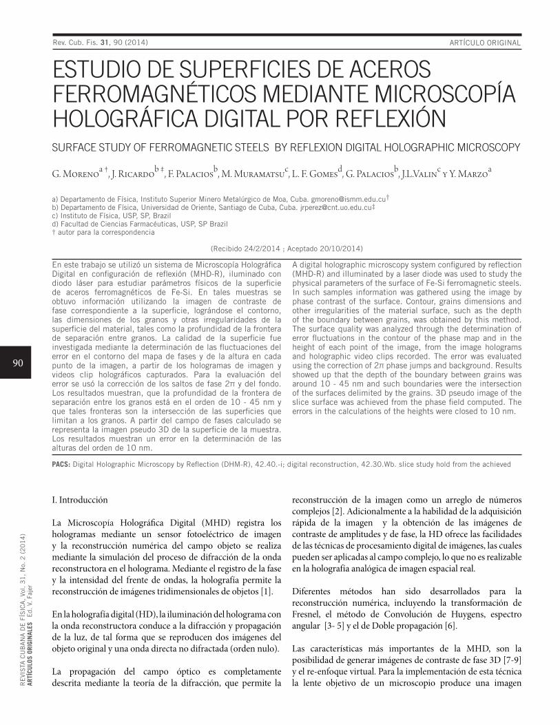
90

RE

VIS

TA C

UB

AN

A D

E F

ÍSIC

A,

Vol. 3

1,

No.

2 (

20

14

)AR

TÍCU

LOS

ORIG

INAL

ESE

d. V

. Fa

jer

ARTÍCULO ORIGINAL

ESTUDIO DE SUPERFICIES DE ACEROS FERROMAGNÉTICOS MEDIANTE MICROSCOPÍA HOLOGRÁFICA DIGITAL POR REFLEXIÓNSURFACE STUDY OF FERROMAGNETIC STEELS BY REFLEXION DIGITAL HOLOGRAPHIC MICROSCOPY

G. Morenoa †, J. Ricardob ‡, F. Palaciosb, M. Muramatsuc, L. F. Gomesd, G. Palaciosb, J.L.Valinc y Y. Marzoa

a) Departamento de Física, Instituto Superior Minero Metalúrgico de Moa, Cuba. gmoreno@ismm.edu.cu†b) Departamento de Física, Universidad de Oriente, Santiago de Cuba, Cuba. jrperez@cnt.uo.edu.cu‡ c) Instituto de Física, USP, SP, Brazild) Facultad de Ciencias Farmacéuticas, USP, SP Brazil† autor para la correspondencia

(Recibido 24/2/2014 ; Aceptado 20/10/2014)

En este trabajo se utilizó un sistema de Microscopía Holográfica Digital en configuración de reflexión (MHD-R), iluminado con diodo láser para estudiar parámetros físicos de la superficie de aceros ferromagnéticos de Fe-Si. En tales muestras se obtuvo información utilizando la imagen de contraste de fase correspondiente a la superficie, lográndose el contorno, las dimensiones de los granos y otras irregularidades de la superficie del material, tales como la profundidad de la frontera de separación entre granos. La calidad de la superficie fue investigada mediante la determinación de las fluctuaciones del error en el contorno del mapa de fases y de la altura en cada punto de la imagen, a partir de los hologramas de imagen y videos clip holográficos capturados. Para la evaluación del error se usó la corrección de los saltos de fase 2π y del fondo. Los resultados muestran, que la profundidad de la frontera de separación entre los granos está en el orden de 10 - 45 nm y que tales fronteras son la intersección de las superficies que limitan a los granos. A partir del campo de fases calculado se representa la imagen pseudo 3D de la superficie de la muestra. Los resultados muestran un error en la determinación de las alturas del orden de 10 nm.

A digital holographic microscopy system configured by reflection (MHD-R) and illuminated by a laser diode was used to study the physical parameters of the surface of Fe-Si ferromagnetic steels. In such samples information was gathered using the image by phase contrast of the surface. Contour, grains dimensions and other irregularities of the material surface, such as the depth of the boundary between grains, was obtained by this method. The surface quality was analyzed through the determination of error fluctuations in the contour of the phase map and in the height of each point of the image, from the image holograms and holographic video clips recorded. The error was evaluated using the correction of 2π phase jumps and background. Results showed up that the depth of the boundary between grains was around 10 - 45 nm and such boundaries were the intersection of the surfaces delimited by the grains. 3D pseudo image of the slice surface was achieved from the phase field computed. The errors in the calculations of the heights were closed to 10 nm.

PACS: Digital Holographic Microscopy by Reflection (DHM-R), 42.40.-i; digital reconstruction, 42.30.Wb. slice study hold from the achieved

I. Introducción

La Microscopía Holográfica Digital (MHD) registra los hologramas mediante un sensor fotoeléctrico de imagen y la reconstrucción numérica del campo objeto se realiza mediante la simulación del proceso de difracción de la onda reconstructora en el holograma. Mediante el registro de la fase y la intensidad del frente de ondas, la holografía permite la reconstrucción de imágenes tridimensionales de objetos [1].

En la holografía digital (HD), la iluminación del holograma con la onda reconstructora conduce a la difracción y propagación de la luz, de tal forma que se reproducen dos imágenes del objeto original y una onda directa no difractada (orden nulo). La propagación del campo óptico es completamente descrita mediante la teoría de la difracción, que permite la

reconstrucción de la imagen como un arreglo de números complejos [2]. Adicionalmente a la habilidad de la adquisición rápida de la imagen y la obtención de las imágenes de contraste de amplitudes y de fase, la HD ofrece las facilidades de las técnicas de procesamiento digital de imágenes, las cuales pueden ser aplicadas al campo complejo, lo que no es realizable en la holografía analógica de imagen espacial real.

Diferentes métodos han sido desarrollados para la reconstrucción numérica, incluyendo la transformación de Fresnel, el método de Convolución de Huygens, espectro angular [3- 5] y el de Doble propagación [6].

Las características más importantes de la MHD, son la posibilidad de generar imágenes de contraste de fase 3D [7-9] y el re-enfoque virtual. Para la implementación de esta técnica la lente objetivo de un microscopio produce una imagen

Rev. Cub. Fis. 31, 90 (2014)

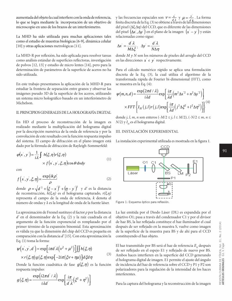
91

RE

VIS

TA C

UB

AN

A D

E F

ÍSIC

A,

Vol. 3

1,

No.

2 (

20

14

)AR

TÍCU

LOS

ORIG

INAL

ESE

d. V

. Fa

jer

aumentada del objeto la cual interfiere con la onda de referencia, lo que se logra mediante la incorporación de un objetivo de microscopio en uno de los brazos de un interferómetro.

La MHD ha sido utilizada para muchas aplicaciones tales como el estudio de muestras biológicas [6-9], dinámica celular [10] y otras aplicaciones metrológicas [11].

La MHD-R por reflexión, ha sido aplicada para resolver tareas como análisis estándar de superficies reflectoras, investigación de polvos [12, 13] y estudio de micro lentes [14], pero para la determinación de parámetros de la superficie de aceros no ha sido utilizada.

En este trabajo presentamos la aplicación de la MHD-R para estudiar la frontera de separación entre granos y observar las imágenes pseudo 3D de la superficie de los aceros, utilizando un sistema micro holográfico basado en un interferómetro de Michelson.

II. PRINCIPIOS GENERALES DE LA HOLOGRAFÍA DIGITAL

En HD el proceso de reconstrucción de la imagen es realizado mediante la multiplicación del holograma digital por la descripción numérica de la onda de referencia y por la convolución de este resultado con la función respuesta impulso del sistema. El campo de difracción en el plano imagen está dado por la fórmula de difracción de Rayleigh-Sommerfeld:

( ) ( ) ( )

( ) dxdyyxf

rhi

yx

θηξ

ηξηξλ

ϕ

cos,,,

,,1,

''

''

×

= ∫∫

(1)

con

( ) ( )' ' exp, , ,

ikf x y

ρξ η

ρ=

(2)

donde ( ) ( )2'2'2' yxd −+−+= ηξρ y d' es la distancia de reconstrucción, h(ξ,η) es el holograma capturado, r(ξ,η) representa el campo de la onda de referencia, k denota el número de ondas y λ es la longitud de onda de la fuente láser. La aproximación de Fresnel sustituye el factor ρ por la distancia d' en el denominador de la Eq. (2) y la raíz cuadrada en el argumento de la función exponencial es remplazado por el primer término de la expansión binomial. Esta aproximación es válida ya que la dimensión del chip del CCD es pequeña en comparación con la distancia d' [15]. Con esta aproximación la Eq. (1) toma la forma:

( ) ( ) ( )( ) ( ) ( )

' ' ' ' 2 2, , exp ,

, , exp 2

x y d i d h

r g i d d

ψ π λ ν µ ξ η

ξ η ξ η π ξν ηµ ξ η

= + × − +

∫∫

(3)

Donde la función cuadrática de fase ( )ηξ ,g es la función respuesta impulso:

( ) ( ) ( )'

2 2' '

exp 2 /, exp

i d igi d d

π λ πξ η ξ ηλ λ

= +

y las frecuencias espaciales son '

'x

d λν = y

'

'y

d λµ = . La forma

finita discreta de la Eq. (3) se obtiene a través de las dimensiones del pixel (∆ξ,∆η) del CCD, que es diferente de las dimensiones del pixel ( )'' , yx ∆∆ en el plano de la imagen ( )'' yx − y están relacionadas como sigue:

ξλ

∆=∆

Mdx

''

; η

λ∆

=∆Ndy

''

donde M y N son los números de pixeles del arreglo del CCD en las direcciones 'x e 'y respectivamente.

Para el cálculo numérico rápido se aplica una formulación discreta de la Eq. (3), la cual utiliza el algoritmo de la transformada rápida de Fourier bi-dimensional (FFT), como se muestra en la Eq. (4):

( ) ( ) ( )( ) ( ) ( )

2 '2 2 '2

2 2 2 2

exp 2 /, , exp

, , expH

d im n d m x n yi d d

iFFT I j l r j l j ld

π λ πψλ λ

π ξ ηλ

= ∆ + ∆ × ∆ + ∆

(4)

donde j, l, m, n son enteros (-M/2 ≤ j, l ≤ M/2), (-N/2 ≤ m, n ≤ N/2) y IH es el holograma digital.

III. INSTALACIÓN EXPERIMENTAL

La instalación experimental utilizada es mostrada en la figura 1.

Figura 1: Esquema óptico para reflexión.

La luz emitida por el Diodo Láser (DL) es expandida por el objetivo O1; pasa a través del condensador C1 y por el divisor de haz BS, la luz reflejada constituye el haz iluminador el cual después de ser reflejado en la muestra S, vuelve como imagen de la superficie de la muestra para BS y de ahí para el CCD constituyendo el haz objeto.

El haz transmitido por BS será el haz de referencia ER después de ser reflejado en el espejo E1 y reflejado de nuevo por BS. Ambos haces interfieren en la superficie del CCD generando el holograma digital de imagen. E1 permite el ajuste del ángulo de incidencia del haz de referencia sobre el CCD y P1 y P2 son polarizadores para la regulación de la intensidad de los haces interferentes.

Para la captura del holograma y la reconstrucción de la imagen

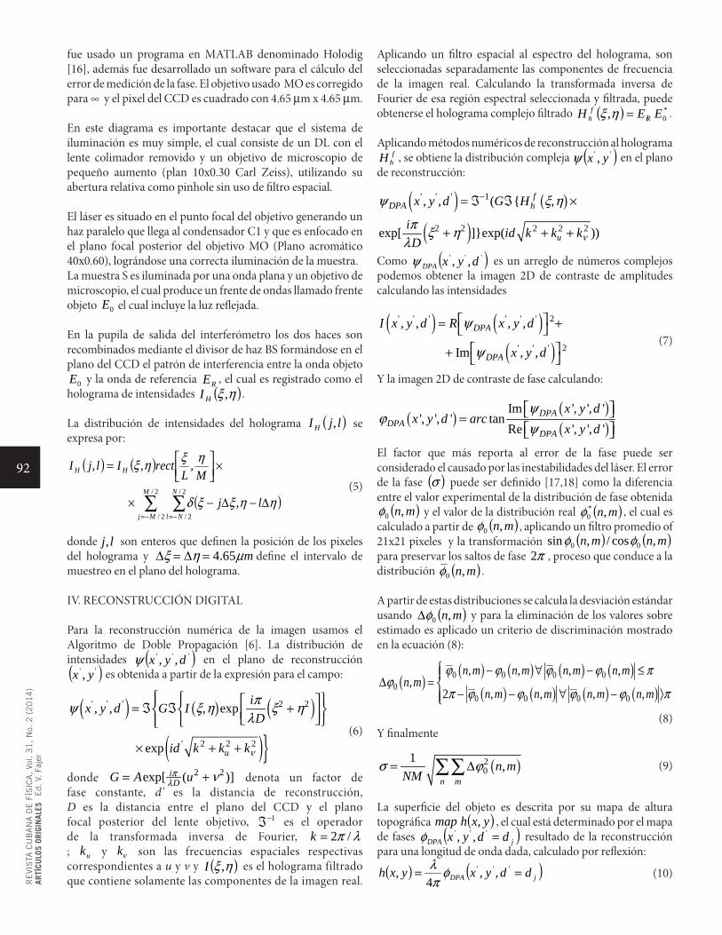
92

RE

VIS

TA C

UB

AN

A D

E F

ÍSIC

A,

Vol. 3

1,

No.

2 (

20

14

)AR

TÍCU

LOS

ORIG

INAL

ESE

d. V

. Fa

jer

fue usado un programa en MATLAB denominado Holodig [16], además fue desarrollado un software para el cálculo del error de medición de la fase. El objetivo usado MO es corregido para ∞

y el pixel del CCD es cuadrado con 4.65 µm x 4.65 µm.

En este diagrama es importante destacar que el sistema de iluminación es muy simple, el cual consiste de un DL con el lente colimador removido y un objetivo de microscopio de pequeño aumento (plan 10x0.30 Carl Zeiss), utilizando su abertura relativa como pinhole sin uso de filtro espacial.

El láser es situado en el punto focal del objetivo generando un haz paralelo que llega al condensador C1 y que es enfocado en el plano focal posterior del objetivo MO (Plano acromático 40x0.60), lográndose una correcta iluminación de la muestra.La muestra S es iluminada por una onda plana y un objetivo de microscopio, el cual produce un frente de ondas llamado frente objeto 0E el cual incluye la luz reflejada.

En la pupila de salida del interferómetro los dos haces son recombinados mediante el divisor de haz BS formándose en el plano del CCD el patrón de interferencia entre la onda objeto

0E y la onda de referencia RE , el cual es registrado como el holograma de intensidades ( )ηξ ,HI .

La distribución de intensidades del holograma ( )ljI H , se expresa por:

( ) ( )

( )∑ ∑−= −=

∆−∆−×

×

=

2/

2/

2/

2/,

,,,

M

Mj

N

Nl

HH

lj

MLrectIljI

ηηξξδ

ηξηξ

(5)

donde lj, son enteros que definen la posición de los pixeles del holograma y 4.65 mξ η µ∆ = ∆ = define el intervalo de muestreo en el plano del holograma.

IV. RECONSTRUCCIÓN DIGITAL

Para la reconstrucción numérica de la imagen usamos el Algoritmo de Doble Propagación [6]. La distribución de intensidades ( )''' ,, dyxψ en el plano de reconstrucción ( )'' , yx es obtenida a partir de la expresión para el campo:

( ) ( ) ( )

( )' ' ' 2 2

' 2 2 2

, , , exp

exp u

ix y d G ID

id k k kν

πψ ξ η ξ ηλ

= ℑ ℑ +

× + +

(6)

donde 2 2exp[ ( )]iDG A uπ

λ ν= + denota un factor de fase constante, d' es la distancia de reconstrucción, D es la distancia entre el plano del CCD y el plano focal posterior del lente objetivo, 1−ℑ es el operador de la transformada inversa de Fourier, λπ /2=k; uk y νk son las frecuencias espaciales respectivas correspondientes a u y v y ( )ηξ ,I es el holograma filtrado que contiene solamente las componentes de la imagen real.

Aplicando un filtro espacial al espectro del holograma, son seleccionadas separadamente las componentes de frecuencia de la imagen real. Calculando la transformada inversa de Fourier de esa región espectral seleccionada y filtrada, puede obtenerse el holograma complejo filtrado ( ) *

0, EEH Rlf

h =ηξ .

Aplicando métodos numéricos de reconstrucción al holograma f

hH , se obtiene la distribución compleja ( )'' , yxψ en el plano de reconstrucción:

( ) ( )

( )

' ' ' 1

2 2 2 2 2

, , ( ,

exp[ ]exp( ))

fDPA h

u

x y d G H

i id k k kD ν

ψ ξ η

π ξ ηλ

−= ℑ ℑ ×

+ + +

Como ( )''' ,, dyxDPAψ es un arreglo de números complejos podemos obtener la imagen 2D de contraste de amplitudes calculando las intensidades

( ) ( )( )

' ' ' ' ' ' 2

' ' ' 2

, , , ,

Im , ,

DPA

DPA

I x y d R x y d

x y d

ψ

ψ

= + +

(7)

Y la imagen 2D de contraste de fase calculando:

( ) ( )( )

Im ', ', '', ', ' tan

Re ', ', 'DPA

DPADPA

x y dx y d arc

x y dψ

ϕψ

=

El factor que más reporta al error de la fase puede ser considerado el causado por las inestabilidades del láser. El error de la fase ( )σ puede ser definido [17,18] como la diferencia entre el valor experimental de la distribución de fase obtenida

( )mn,0φ y el valor de la distribución real ( )mn,*0φ , el cual es

calculado a partir de ( )mn,0φ , aplicando un filtro promedio of 21x21 pixeles y la transformación ( ) ( )mnmn ,cos/,sin 00 φφ para preservar los saltos de fase π2 , proceso que conduce a la distribución ( )mn,0φ .

A partir de estas distribuciones se calcula la desviación estándar usando ( )mn,0φ∆ y para la eliminación de los valores sobre estimado es aplicado un criterio de discriminación mostrado en la ecuación (8):

( )( ) ( ) ( ) ( )

( ) ( ) ( ) ( )0 0 0 0

00 0 0 0

, , , ,,

2 , , , ,

n m n m n m n mn m

n m n m n m n m

ϕ ϕ ϕ ϕ πϕ

π ϕ ϕ ϕ ϕ π

− ∀ − ≤∆ = − − ∀ − ⟩

(8)Y finalmente

( )20

1 ,n m

n mNM

σ ϕ= ∆∑∑

(9)

La superficie del objeto es descrita por su mapa de altura topográfica ( )yxhmap , , el cual está determinado por el mapa de fases ( )jDPA ddyx =''' ,,φ resultado de la reconstrucción para una longitud de onda dada, calculado por reflexión:

( ) ( )jDPA ddyxyxh == ''' ,,4

, φπλ

(10)

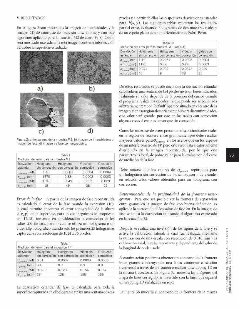
93

RE

VIS

TA C

UB

AN

A D

E F

ÍSIC

A,

Vol. 3

1,

No.

2 (

20

14

)AR

TÍCU

LOS

ORIG

INAL

ESE

d. V

. Fa

jer

V. RESULTADOS

En la figura 2 son mostradas la imagen de intensidades y la imagen 2D de contraste de fases sin unwrapping y con este algoritmo aplicado para la muestra M2 de acero Fe-Si. Como será mostrado más adelante esta imagen contiene información 3D sobre la superficie estudiada.

Figure 2: a) holograma de la muestra M2; b) imagen de intensidades; c) imagen de fase; d) imagen de fase con unwrapping.

Tabla IMedición del error para la muestra M1Desviaciónestándar

Holograma sin corrección

Holograma con corrección

Video sin corrección

Video con corrección

σgeneral-Ф (rad) 1.48 0.0003 0.0004 0.0004σgeneral-h (nm) 1470 0.33 0.0003 0.0003σgeneral-Ф (rad) 0.018 0.049 0.033 0.029σgeneral-h (nm) 18 49 38 26

Error de la fase A partir de la imagen de fase reconstruida es calculado el error de la fase usando la expresión (10), la cual permite encontrar el error topográfico de la altura

( )yxh , de la superficie, para lo cual seguimos lo propuesto en [17,18], tomando en consideración la corrección de los saltos π2 de fase, para lo cual se utiliza un holograma o un video clip holográfico usando solo los primeros 25 hologramas capturados con resolución de 1024 x 76 pixeles.

Tabla IIMedición del error para el espejo de FPDesviación estándar

Holograma sin corrección

Holograma con corrección

Video sin corrección

Video con corrección

σgeneral-Ф (rad) 0.31 0.0007 0.0008 0.0008

σgeneral-h (nm) 308 0.7 0.9 0.9

σgeneral-Ф (rad) 0.023 0.129 0.156 0.157σgeneral-h (nm) 28 128 155 156

La desviación estándar de fase, es calculada para toda la superficie capturada en el holograma y para una ventana de 4 x 4

pixeles y a partir de ellas las respectivas desviaciones estándar para ( )yxh , . Las siguientes tablas muestran los resultados para el error, evaluando hologramas de dos muestras reales y de un espejo plano de un interferómetro de Fabri-Perot.

Tabla IIIMedición del error para la muestra M1 (zona-3)Desviación estándar

Holograma sin corrección

Holograma con corrección

Video sin corrección

Video con corrección

σgeneral-Ф (rad) 1.19 0.0034 0.0003 0.0004σgeneral-h (nm) 1185 0.32 0.29 0.0003σgeneral-Ф (rad) 0.041 0.009 0.0378 0.029σgeneral-h (nm) 40 9 38 26

De estos resultados se puede decir que la desviación estándar calculada en una ventana de 4x4 pixeles no es un buen indicador, realmente su valor depende de la posición del cursor cuando el programa realiza los cálculos, la que puede ser seleccionada arbitrariamente y por “default” aparece situado en el centro de la imagen, si en esa región aleatoriamente hubiera discontinuidades, este valor será grande, por esto en las tablas con corrección algunas veces el error es mayor que sin corrección.

Como las muestras de acero presentan discontinuidades reales en la región de frontera entre granos, siempre debe resultar mayores valores para windowsσ en los aceros que en los espejos de un interferómetro de FP, pero este error esta aleatoriamente distribuido en la imagen reconstruida, por lo que este parámetro es local, de pobre valor para la evaluación del error de medición de la fase.

Debe notarse que los valores de generalσ reportados para un holograma sin corrección de los saltos, son muy grandes en relación a los valores obtenidos para un holograma con corrección.

Determinación de la profundidad de la frontera inter-granos Para que sea posible ver la frontera de separación entre granos en la imagen de fase con buena definición, es aplicada la corrección de los saltos de fase 2π. En la imagen de fase se aplica la corrección utilizando el algoritmo expresado en la ecuación (8).

Después se realiza una inversión de los signos de la fase y se activa la calibración lateral, la cual fue realizada mediante la utilización de una escala con resolución de 0.010 mm y la calibración axial, la más importante y dependiente del valor de la longitud de onda usada.

A continuación podemos obtener un contorno de la frontera inter granos construyendo una línea contorno o sección transversal a través de la frontera o realizar unwrapping 1D en la misma trayectoria. La Figura 3a muestra las imágenes del mapa de fases corregido he invertido con la línea que sigue el unwrapping 1D señalizada en rojo.

La Figura 3b muestra el contorno de la frontera en la misma

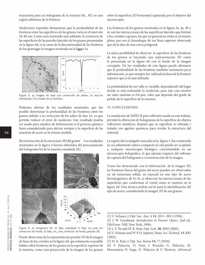
94

RE

VIS

TA C

UB

AN

A D

E F

ÍSIC

A,

Vol. 3

1,

No.

2 (

20

14

)AR

TÍCU

LOS

ORIG

INAL

ESE

d. V

. Fa

jer

trayectoria para un holograma de la muestra h6_ M2 en una región arbitraria de la frontera.

Mediciones repetidas demuestran que la profundidad de las fronteras entre las superficies de los granos varía en el intervalo 10-40 nm. Como será mostrado más adelante, la existencia de las superficies de las paredes laterales de los granos presentadas en la figura 4d, es la causa de la discontinuidad de las fronteras de los granos en la imagen mostrada en la figura 3a.

Figura 3: a) imagen de fase con corrección de saltos; b) sección transversal 1D a través de la frontera.

Podemos afirmar de los resultados mostrados, que fue posible determinar la profundidad de las fronteras entre los granos debido a la corrección de los saltos de fase 2π, ya que permite reducir el error de medición. Este resultado podría ser usado para estudios de deformación si el proceso químico fuera estandarizado para afectar siempre a la superficie de las muestras de acero en la misma medida.

Reconstrucción de la estructura 3D del grano Los resultados mostrados en la figura 4 fueron obtenidos del procesamiento del holograma h4 de la muestra estudiada M2.

Figura 4: a) holograma h4; b) fase unwraped c) fase inv_unw_con correccion de fondo; d) fase_inv_unw_correcion de fondo_pseudo 3D.

Puede observarse de la representación pseudo 3D de la imagen de fases de los cristales en la figura 4d, que solamente es posible hablar sobre fronteras de los granos en la superficie superior de la muestra, como una proyección de la imagen de los granos

b)a)

sobre la superficie 2D horizontal capturada por el objetivo del microscopio.

Las fronteras de los granos mostradas en la figura 3a, 4a, 4b y 4c son las intersecciones de las superficies laterales que limitan a los cristales o granos, las que en general no están en el mismo plano, por eso el desenfoque de esa línea superior observada que da la idea de una curva poligonal.

La única posibilidad de observar la superficie de las fronteras de los granos es haciendo una representación 3D como la presentada en la figura 4d con el fondo de la imagen corregido. De los resultados de esta figura puede afirmarse que la profundidad de las fronteras medidas suministra poca información, ya que siempre fue utilizada la línea de la frontera superior que es la más definida.

La profundidad de ese valle es variable, dependiendo del lugar donde se está realizando la medición, para este caso mostró un valor máximo es 0.8 µm, valor que depende del grado de pulido de la superficie de la muestra.

VI. CONCLUSIONES

La instalación de MHD-R para reflexión usada en este trabajo, permite la obtención de hologramas de la superficie de objetos reflectores metálicos, después que su superficie es refinada y tratada con agentes químicos para revelar la estructura del material.

La región del rectángulo marcada en la figura 1, fue construida en un aditamento óptico compacto el cual puede ser acoplado a cualquier microscopio biológico convirtiéndolo en un microscopio holográfico, el que además requiere del software de captura del holograma y reconstrucción de la imagen.

Como fue demostrado con la información de la imagen 3D, las fronteras físicas del grano del acero pueden ser observadas en tal estructura sólida, en especial en este tipo de acero ferromagnético de Fe-Si, se observan las intersecciones de las superficies que conforman al cristal como se muestra en la figura 4d. Esta técnica podría servir para la identificación del tipo de acero, considerando la imagen 3D de sus granos.

[1] U. Schnars, J. Opt. Soc. Am. A 11, 2011–2015 (1994).[2] J. W. Goodman, Introduction to Fourier Optics, 2nd ed., (McGraw- Hill, New York, 1996). [3] L. F. Yu and M. K. Kim, Opt. Lett. 30, 2092 (2005). [4] U. Schnars and W. P. O. Juptner, Meas. Sci. Technol. 13, R85 (2002). [5] M. K. Kim, J. Opt. Soc. Korea 14, 77 (2010). [6] F. Palacios, O. Font, J. Ricardo, G. Palacios, M. Muramatsu D. Soga, D. Palacios & F. Monroy, Advanced

95

RE

VIS

TA C

UB

AN

A D

E F

ÍSIC

A,

Vol. 3

1,

No.

2 (

20

14

)AR

TÍCU

LOS

ORIG

INAL

ESE

d. V

. Fa

jer

Holography - Metrology and Imaging, (InTech, 2011), Chap. 9, pp. 183-206.[7] G. Popescu, L.Deflores, J. Vaughan, K. Badizadegan, H. Iwai, R. Dasari & M. Feld, Opt. Lett. 29, 2503 (2004).[8] F. Palacios, J. Ricardo, G. Palacios, E. Gonçalves, J. Valin & R. De Souza, Opt. Commun. 248, 41 (2005).[9] J. Ricardo, et al., J. Phys. Conf. Ser. 274, 012066 (2011). [10] P. Marquet, et al., Proc. SPIE 6191, 61910U (2006).[11] E. Novak, Proc. SPIE 5716, 173 (2005). [12] A. Khmaladze, A. Restrepo, M. Kim, R. Castañeda & A. Blandón, Applied Optics 47, 3203 (2008).[13] Y. Wu, X. Wu Z. Wang, L. Chen and K. Cen, Applied Optics 50, H22 (2011). [14] F. Charrière, et al., Applied Optics 45, 829 (2006).

[15] F. Palacios, Oneida Font, Jorge Ricardo, Guillermo Palacios, Mikiya Muramatsu, Diogo Soga, Daniel Palacios, José Valin and Freddy Monroy, (2011), in Advanced Holography - Metrology and Imaging, Ed. by I. Naydenova, ISBN 978-953-307-729-1,184-206: http://www.intechopen.com/articles/show/title/alternative-reconstruction-method-and-object-analysis-in-digital-holographic-microscopy.[16] J. L. Valin, E. Gonçalves, F. Palacios and J. Ricardo Perez, Opt. Lasers Eng. 4, 99 (2005). [17] C. Remmersmann, et al., Appl. Opt. 48, 1463 (2009).[18] F. Montfort, et al., Surface roughness parameters measurements by digital holographic microscopy, in 3rd Int. Symp. on Precision Mechanical Measurements (Xinjiang, 2006).

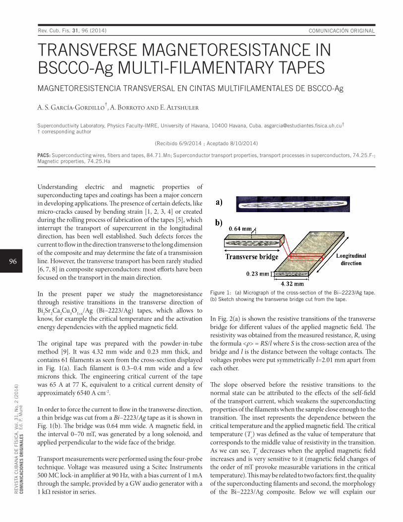
96

RE

VIS

TA C

UB

AN

A D

E F

ÍSIC

A,

Vol. 3

1,

No.

2 (

20

14

)CO

MU

NIC

ACIO

NES

ORI

GIN

ALES

E

d. P

. M

uné

COMUNICACIÓN ORIGINAL

TRANSVERSE MAGNETORESISTANCE IN BSCCO-Ag MULTI-FILAMENTARY TAPESMAGNETORESISTENCIA TRANSVERSAL EN CINTAS MULTIFILAMENTALES DE BSCCO-Ag

A. S. García-Gordillo†, A. Borroto and E. Altshuler

Superconductivity Laboratory, Physics Faculty-IMRE, University of Havana, 10400 Havana, Cuba. asgarcia@estudiantes.fisica.uh.cu†† corresponding author

(Recibido 6/9/2014 ; Aceptado 8/10/2014)

PACS: Superconducting wires, fibers and tapes, 84.71.Mn; Superconductor transport properties, transport processes in superconductors, 74.25.F-; Magnetic properties, 74.25.Ha

Understanding electric and magnetic properties of superconducting tapes and coatings has been a major concern in developing applications. The presence of certain defects, like micro-cracks caused by bending strain [1, 2, 3, 4] or created during the rolling process of fabrication of the tapes [5], which interrupt the transport of supercurrent in the longitudinal direction, has been well established. Such defects forces the current to flow in the direction transverse to the long dimension of the composite and may determine the fate of a transmission line. However, the transverse transport has been rarely studied [6, 7, 8] in composite superconductors: most efforts have been focused on the transport in the main direction.

In the present paper we study the magnetoresistance through resistive transitions in the transverse direction of Bi2Sr2Ca2Cu3O1+x/Ag (Bi−2223/Ag) tapes, which allows to know, for example the critical temperature and the activation energy dependencies with the applied magnetic field.

The original tape was prepared with the powder-in-tube method [9]. It was 4.32 mm wide and 0.23 mm thick, and contains 61 filaments as seen from the cross-section displayed in Fig. 1(a). Each filament is 0.3−0.4 mm wide and a few microns thick. The engineering critical current of the tape was 65 A at 77 K, equivalent to a critical current density of approximately 6540 A cm-2.

In order to force the current to flow in the transverse direction, a thin bridge was cut from a Bi−2223/Ag tape as it is shown in Fig. 1(b). The bridge was 0.64 mm wide. A magnetic field, in the interval 0–70 mT, was generated by a long solenoid, and applied perpendicular to the wide face of the bridge.

Transport measurements were performed using the four-probe technique. Voltage was measured using a Scitec Instruments 500 MC lock-in amplifier at 90 Hz, with a bias current of 1 mA through the sample, provided by a GW audio generator with a 1 kΩ resistor in series.

Figure 1: (a) Micrograph of the cross-section of the Bi−2223/Ag tape. (b) Sketch showing the transverse bridge cut from the tape.

In Fig. 2(a) is shown the resistive transitions of the transverse bridge for different values of the applied magnetic field. The resistivity was obtained from the measured resistance, R, using the formula <ρ> = RS/l where S is the cross-section area of the bridge and l is the distance between the voltage contacts. The voltages probes were put symmetrically l=2.01 mm apart from each other.

The slope observed before the resistive transitions to the normal state can be attributed to the effects of the self-field of the transport current, which weakens the superconducting properties of the filaments when the sample close enough to the transition. The inset represents the dependence between the critical temperature and the applied magnetic field. The critical temperature (Tc) was defined as the value of temperature that corresponds to the middle value of resistivity in the transition. As we can see, Tc decreases when the applied magnetic field increases and is very sensitive to it (magnetic field changes of the order of mT provoke measurable variations in the critical temperature). This may be related to two factors: first, the quality of the superconducting filaments and second, the morphology of the Bi−2223/Ag composite. Below we will explain our

Rev. Cub. Fis. 31, 96 (2014)

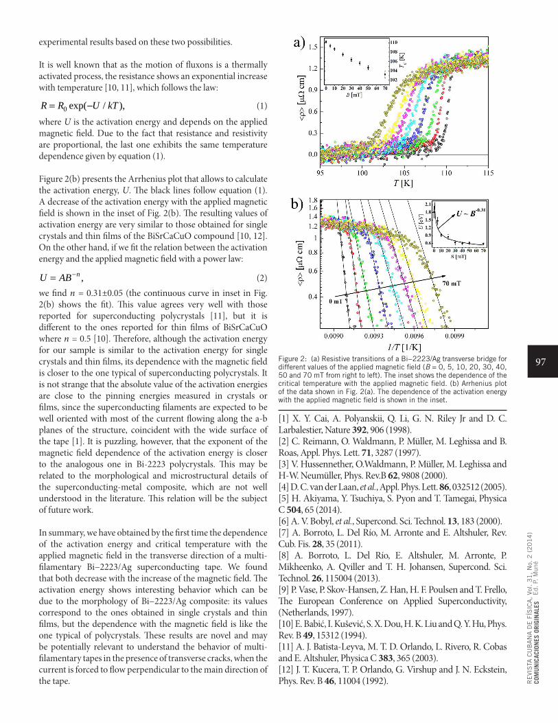
97

RE

VIS

TA C

UB

AN

A D

E F

ÍSIC

A,

Vol. 3

1,

No.

2 (

20

14

)CO

MU

NIC

ACIO

NES

ORI

GIN

ALES

E

d. P

. M

uné

experimental results based on these two possibilities.

It is well known that as the motion of fluxons is a thermally activated process, the resistance shows an exponential increase with temperature [10, 11], which follows the law:

0 exp( / ),R R U kT= − (1)

where U is the activation energy and depends on the applied magnetic field. Due to the fact that resistance and resistivity are proportional, the last one exhibits the same temperature dependence given by equation (1).

Figure 2(b) presents the Arrhenius plot that allows to calculate the activation energy, U. The black lines follow equation (1). A decrease of the activation energy with the applied magnetic field is shown in the inset of Fig. 2(b). The resulting values of activation energy are very similar to those obtained for single crystals and thin films of the BiSrCaCuO compound [10, 12]. On the other hand, if we fit the relation between the activation energy and the applied magnetic field with a power law:

,nU AB−= (2)we find n = 0.31±0.05 (the continuous curve in inset in Fig. 2(b) shows the fit). This value agrees very well with those reported for superconducting polycrystals [11], but it is different to the ones reported for thin films of BiSrCaCuO where n = 0.5 [10]. Therefore, although the activation energy for our sample is similar to the activation energy for single crystals and thin films, its dependence with the magnetic field is closer to the one typical of superconducting polycrystals. It is not strange that the absolute value of the activation energies are close to the pinning energies measured in crystals or films, since the superconducting filaments are expected to be well oriented with most of the current flowing along the a-b planes of the structure, coincident with the wide surface of the tape [1]. It is puzzling, however, that the exponent of the magnetic field dependence of the activation energy is closer to the analogous one in Bi-2223 polycrystals. This may be related to the morphological and microstructural details of the superconducting-metal composite, which are not well understood in the literature. This relation will be the subject of future work.

In summary, we have obtained by the first time the dependence of the activation energy and critical temperature with the applied magnetic field in the transverse direction of a multi-filamentary Bi−2223/Ag superconducting tape. We found that both decrease with the increase of the magnetic field. The activation energy shows interesting behavior which can be due to the morphology of Bi−2223/Ag composite: its values correspond to the ones obtained in single crystals and thin films, but the dependence with the magnetic field is like the one typical of polycrystals. These results are novel and may be potentially relevant to understand the behavior of multi-filamentary tapes in the presence of transverse cracks, when the current is forced to flow perpendicular to the main direction of the tape.

Figure 2: (a) Resistive transitions of a Bi−2223/Ag transverse bridge for different values of the applied magnetic field (B = 0, 5, 10, 20, 30, 40, 50 and 70 mT from right to left). The inset shows the dependence of the critical temperature with the applied magnetic field. (b) Arrhenius plot of the data shown in Fig. 2(a). The dependence of the activation energy with the applied magnetic field is shown in the inset.

[1] X. Y. Cai, A. Polyanskii, Q. Li, G. N. Riley Jr and D. C. Larbalestier, Nature 392, 906 (1998).[2] C. Reimann, O. Waldmann, P. Müller, M. Leghissa and B. Roas, Appl. Phys. Lett. 71, 3287 (1997).[3] V. Hussennether, O.Waldmann, P. Müller, M. Leghissa and H-W. Neumüller, Phys. Rev.B 62, 9808 (2000).[4] D. C. van der Laan, et al., Appl. Phys. Lett. 86, 032512 (2005).[5] H. Akiyama, Y. Tsuchiya, S. Pyon and T. Tamegai, Physica C 504, 65 (2014).[6] A. V. Bobyl, et al., Supercond. Sci. Technol. 13, 183 (2000).[7] A. Borroto, L. Del Río, M. Arronte and E. Altshuler, Rev. Cub. Fis. 28, 35 (2011).[8] A. Borroto, L. Del Río, E. Altshuler, M. Arronte, P. Mikheenko, A. Qviller and T. H. Johansen, Supercond. Sci. Technol. 26, 115004 (2013).[9] P. Vase, P. Skov-Hansen, Z. Han, H. F. Poulsen and T. Frello, The European Conference on Applied Superconductivity, (Netherlands, 1997).[10] E. Babić, I. Kušević, S. X. Dou, H. K. Liu and Q. Y. Hu, Phys. Rev. B 49, 15312 (1994).[11] A. J. Batista-Leyva, M. T. D. Orlando, L. Rivero, R. Cobas and E. Altshuler, Physica C 383, 365 (2003).[12] J. T. Kucera, T. P. Orlando, G. Virshup and J. N. Eckstein, Phys. Rev. B 46, 11004 (1992).

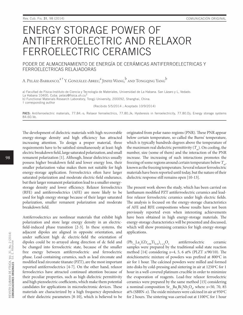
98

RE

VIS

TA C

UB

AN

A D

E F

ÍSIC

A,

Vol. 3

1,

No.

2 (

20

14

)CO

MU

NIC

ACIO

NES

ORI

GIN

ALES

E

d. E

. A

ltsh

uler

COMUNICACIÓN ORIGINAL

ENERGY STORAGE POWER OF ANTIFERROELECTRIC AND RELAXOR FERROELECTRIC CERAMICSPODER DE ALMACENAMIENTO DE ENERGÍA DE CERÁMICAS ANTIFERROELECTRICAS Y FERROELECTRICAS RELAJADORAS

A. Peláiz-Barranco,a † Y. González-Abreu,a Jinfei Wang,b and Tongqing Yangb

a) Facultad de Física-Instituto de Ciencia y Tecnología de Materiales, Universidad de La Habana. San Lázaro y L, Vedado.La Habana 10400, Cuba. pelaiz@fisica.uh.cu†b) Functional Materials Research Laboratory, Tongji University, 200092, Shanghai, China.† corresponding author

(Recibido 5/5/2014 ; Aceptado 10/9/2014)

PACS: Antiferroelectric materials, 77.84.-s; Relaxor ferroelectrics, 77.80.Jk; Hysteresis in ferroelectricity, 77.80.Dj; Energy storage systems 84.60.Ve.

The development of dielectric materials with high recoverable energy-storage density and high efficiency has attracted increasing attention. To design a proper material, three requirements have to be satisfied simultaneously at least: high electric breakdown field, large saturated polarization, and small remanent polarization [1]. Although, linear dielectrics usually possess higher breakdown field and lower energy loss, their smaller polarization value makes them not suitable for high energy-storage application. Ferroelectrics often have larger saturated polarization and moderate electric-field endurance, but their larger remanent polarization lead to a smaller energy-storage density and lower efficiency. Relaxor ferroelectrics (RFE) and antiferroelectrics (AFE) are more likely to be used for high energy storage because of their larger saturated polarization, smaller remanent polarization and moderate breakdown field.

Antiferroelectrics are nonlinear materials that exhibit high polarization and store large energy density in an electric-field-induced phase transition [2-3]. In these systems, the adjacent dipoles are aligned in opposite orientation, and under sufficient high dc electric-field the orientation of dipoles could be re-arrayed along direction of dc field and be changed into ferroelectric state, because of the smaller free energy between antiferroelectric and ferroelectric phase. Lead-containing ceramics, such as lead zirconate and modified lead zirconate titanate (PZT), are the most important reported antiferroelectrics [4-7]. On the other hand, relaxor ferroelectrics have attracted continued attention because of their peculiar properties, such as high dielectric permittivity and high piezoelectric coefficients, which make them potential candidates for applications in microelectronic devices. These materials are characterized by a high frequency dependence of their dielectric parameters [8-10], which is believed to be

originated from polar nano-regions (PNR). These PNR appear below certain temperature, so-called the Burns’ temperature, which is typically hundreds degrees above the temperature of the maximum real dielectric permittivity (Tm). On cooling, the number, size (some of them) and the interaction of the PNR increase. The increasing of such interactions promotes the freezing of some regions around certain temperature below Tm, known as the freezing temperature. Several relaxor ferroelectric materials have been reported until today, but the nature of their dielectric response still remains open [10-13].

The present work shows the study, which has been carried on lanthanum modified PZT antiferroelectric ceramics and lead-free relaxor ferroelectric ceramics under high electric fields. The analysis is focused on the energy-storage characteristics of AFE and RFE compositions whose results have not been previously reported even when interesting achievements have been obtained in high energy-storage materials. The energy-storage characteristics will be presented and discussed, which will show promising ceramics for high energy-storage applications.

(Pb1-xLax)(Zr0.90Ti0.10)1-x/4O3 antiferroelectric ceramic samples were prepared by the traditional solid state reaction method [14] considering x=4, 5, 6 at% (PLZT x/90/10). The stoichiometric mixture of powders was prefired at 800oC in air for 1 hour. The calcined powders were milled and formed into disks by cold-pressing and sintering in air at 1250oC for 1 hour in a well-covered platinum crucible in order to minimize the evaporation of reagents. Lead-free relaxor ferroelectric ceramics were prepared by the same method [15] considering a nominal composition Sr1-xBaxBi2Nb2O9, where x=50, 70, 85 at% (SBBN-x). The oxide mixtures were calcined in air at 950oC for 2 hours. The sintering was carried out at 1100oC for 1 hour

Rev. Cub. Fis. 31, 98 (2014)

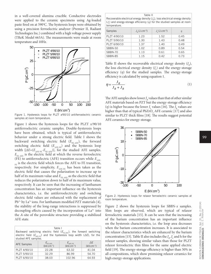
99

RE

VIS

TA C

UB

AN

A D

E F

ÍSIC

A,

Vol. 3

1,

No.

2 (

20

14

)CO

MU

NIC

ACIO

NES

ORI

GIN

ALES

E

d. E

. A

ltsh

uler

in a well-covered alumina crucible. Conductive electrodes were applied to the ceramic specimens using Ag-loaded paste fired on at 590oC. The hysteresis loops were obtained by using a precision ferroelectric analyzer (Premier II, Radiant Technologies Inc.) combined with a high voltage power supply (TReK Model 663A). The measurements were made at room temperature and 10Hz.

-150 -100 -50 0 50 100 150-50

-25

0

25

50

P (µ

C.cm

-2)

E (kV.cm-1)

PLZT 4/90/10 PLZT 5/90/10 PLZT 6/90/10

Figure 1. Hysteresis loops for PLZT x/90/10 antiferroelectric ceramic samples at room temperature.

Figure 1 shows the hysteresis loops for the PLZT x/90/10 antiferroelectric ceramic samples. Double-hysteresis loops have been obtained, which is typical of antiferroelectric behavior under a strong electric field. Table I shows the backward switching electric field (EFE-AFE), the forward switching electric field (EAFE-FE) and the hysteresis loop width [ΔE=(EAFE-FE-EFE-AFE)], for the studied AFE samples. EFE-AFE is the electric field at which the reverse ferroelectric (FE) to antiferroelectric (AFE) transition occurs while EAFE-

FE is the electric field which forces the AFE to FE transition, respectively. For simplicity, EAFE-FE has been taken as the electric field that causes the polarization to increase up to half of its maximum value and EFE-AFE as the electric field that reduces the polarization down to half of its maximum value, respectively. It can be seen that the increasing of lanthanum concentration has an important influence on the hysteresis characteristics, i.e. the antiferroelectricity and switching electric field values are enhanced with the replacement of Pb2+ by La3+ ions. For lanthanum modified PZT materials [4], the stability of the long-range interactions is suppressed by decoupling effects caused by the incorporation of La3+ into the A-site of the perovskite structure providing a stabilized AFE state.

Table IBackward switching electric field (EFE-AFE), the forward switching electric field (EAFE-FE) and the hysteresis loop width (ΔE), for the studied AFE samples.

AFE SamplesEFE-AFE

(kV.cm-1)EAFE-FE

(kV.cm-1)ΔE

(kV.cm-1)PLZT 4/90/10 22.28 63.32 41.04PLZT 5/90/10 32.29 86.99 54.70PLZT 6/90/10 38.03 102.96 64.93

Table IIRecoverable electrical energy density (JR), loss electrical energy density (JL) and energy-storage efficiency (η) for the studied samples at room temperature.

Samples JR (J.cm-3) JL (J.cm-3) η

PLZT 4/90/10 1.23 1.52 0.45PLZT 5/90/10 1.30 1.43 0.48PLZT 6/90/10 1.37 1.40 0.49SBBN-50 1.02 0.89 0.54SBBN-70 1.13 0.61 0.65SBBN-85 1.15 0.42 0.73

Table II shows the recoverable electrical energy density (JR), the loss electrical energy density (JL) and the energy-storage efficiency (η) for the studied samples. The energy-storage efficiency is calculated by using equation 1.

R

R R

JJ J

η =+

(1)

The AFE samples show lower JR values than that of other similar AFE materials based on PZT but the energy-storage efficiency (η) is higher because the lower JL values [16]. The JR values are higher than that of typical PbZrO3 AFE ceramic [17] and also similar to PLZT thick films [18]. The results suggest potential AFE ceramics for energy-storage.

-100 -50 0 50 100-36

-18

0

18

36

P (µ

C.cm

-2)

E (kV.cm-1)

SBBN-50 SBBN-70 SBBN-85

Figure 2. Hysteresis loops for relaxor ferroelectric ceramic samples at room temperature.

Figure 2 shows the hysteresis loops for SBBN-x samples. Slim loops are observed, which are typical of relaxor ferroelectric materials [15]. It can be seen that the increasing of the barium concentration has an important influence on the hysteresis characteristics, i.e. the loop area decreases when the barium concentration increases. It is associated to the relaxor characteristics which are enhanced by the barium concentration [15]. Table II also includes the JR, JL and h for the relaxor samples, showing similar values than those for PLZT relaxor ferroelectric thin films for the same applied electric field [19]. The energy-storage efficiency is higher than 50% in all compositions, which show promising relaxor ceramics for high energy-storage applications.

100

RE

VIS

TA C

UB

AN

A D

E F

ÍSIC

A,

Vol. 3

1,

No.

2 (

20

14

)CO

MU

NIC

ACIO

NES

ORI

GIN

ALES

E

d. E

. A

ltsh

uler

It is known that the bulk ceramic materials show lower breakdown strengths than those in thin films, which prevents the recoverable electrical energy density. Higher values have been achieved in thin film forms but the thickness limitation not always meets the practical requirements. Thus, the development of bulk ceramics continues receiving special attention in order to obtain materials with higher breakdown fields in order to increase the energy-storage density.

As summary, antiferroelectric and relaxor ferroelectric ceramics have been studied under high electric fields. The characteristics of the hysteresis loops have been discussed considering the doping concentration. The energy-storage characteristics have been also analyzed showing high energy-storage efficiency values.

The authors wish to thank to the ICTP for financial support of the Latin-American Network of Ferroelectric Materials. Dr. Peláiz-Barranco would like to thank to Tongji University, Shanghai, China.

[1] N. H. Fletcher, A. D. Hilton and B. W. Ricketts, J. Phys. D: Appl. Phys. 29, 253 (1996).[2] F. Jona, G. Shirane, F. Mazzi and R. Pepinsky, Phys. Rev. 105, 849 (1957).[3] G. Shirane, E. Swaguchi and Y. Takagi, Phys. Rev. 84, 476 (1951).

[4] Y. Xu, Ferroelectric Materials and Their Applications (Elsevier Science Publishers B.V., The Netherlands, 1991).[5] X. Hao, J. Zhou and S. An, J. Am. Ceram. Soc. 94, 1647 (2011).[6] Y. Wang, X. Hao, J. Yang, J. Xu and D. Zhao, J. Appl. Phys. 112, 034105 (2012).[7] M. Ye, Q. Sun, X. Chen, Z. Jiang and F. Wang, J. Am. Ceram. Soc. 95, 1486 (2012).[8] G. Burns and F. H. Dacol, Phys. Rev. B. 28, 2527 (1983).[9] Z. Y. Cheng, R. S. Katiyar, X. Yao and A. S. Bhalla, Phys. Rev. B 57, 8166 (1998).[10] O. García-Zaldívar, A. Peláiz-Barranco, F. Calderón-Piñar, A. Fundora-Cruz, J. D. S. Guerra, D. A. Hall and M. E. Mendoza, J. Phys: Cond. Matt. 20, 445230 (2008).[11] V. V. Shvartsman and D. C. Lupascu, J. Am. Ceram. Soc. 95, 1 (2012).[12] L. E. Cross, Ferroelectrics 151, 305 (1994).[13] A. Bokov and Z.-G., J. Mater. Sci. 41, 31 (2006).[14] A. Peláiz-Barranco, J. D. S. Guerra, O. García-Zaldívar, F. Calderón-Piñar, E. B. Araújo, D. A. Hall, M. E. Mendoza and J. A. Eiras. J. Mat. Sci. 43, 6087 (2008).[15] Y. González-Abreu, A. Peláiz-Barranco, J. D. S. Guerra and P. Saint-Grégoire, Phys. Sta. Sol. (b) 250, 1551 (2013).[16] J. Wang, T. Yang, S. Chen, X. Yao, Functional Materials Letters 7, 1350064 (2014).[17] K. Singh, Ferroelectrics 94, 433 (1989).[18] X. Hao, P. Wang, X. Zhang and J. Xu, Mater. Res. Bull. 48, 84 (2013).[19] X. Hao, Y. Wang, J. Yang, S. An and J. Xu, J. Appl. Phys. 112, 114111 (2012).

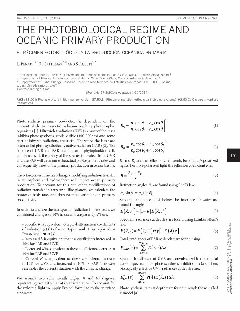
101

RE

VIS

TA C

UB

AN

A D

E F

ÍSIC

A,

Vol. 3

1,

No.

2 (

20

14

)CO

MU

NIC

ACIO

NES

ORI

GIN

ALES

E

ds. A

. Lóp

ez &

E. A

ltsh

uler

COMUNICACIÓN ORIGINAL

THE PHOTOBIOLOGICAL REGIME AND OCEANIC PRIMARY PRODUCTION EL RÉGIMEN FOTOBIOLÓGICO Y LA PRODUCCIÓN OCEÁNICA PRIMARIA

L. Peñate,a † R. Cárdenas b ‡ and S. Agustic *

a) Toxicological Center (CENTOX), Universidad de Ciencias Médicas, Santa Clara, Cuba. liubajc@ucm.vcl.sld.cu†b) Department of Physics, Universidad Central de Las Villas, Santa Clara, Cuba. rcardenas@uclv.edu.cu‡c) Department of Global Change Research, Instituto Mediterráneo de Estudios Avanzados,CSIC – UIB. España. sagusti@imedea.uib-csic.es*† corresponding author

(Recibido 17/2/2014; Aceptado 1/11/2014)

PACS: 88.20.jr Photosynthesis in biomass conversion; 87.50.S- Ultraviolet radiation (effects on biological systems); 92.60.Cc Ocean/atmosphere interactions

Photosynthetic primary production is dependent on the amount of electromagnetic radiation reaching phototrophic organisms [1]. Ultraviolet radiation (UVR) in most of the cases inhibits photosynthesis, while visible (400-700nm) and some part of infrared radiations are useful. Therefore, the latter are often called photosynthetically active radiation (PAR) [2]. The balance of UVR and PAR incident on a phytoplankton cell, combined with the ability of the species to protect from UVR and use PAR will determine the actual photosynthetic rates and consequently most of the primary production in ocean basins. Therefore, environmental changes modifying radiation transfer in atmosphere and hydrosphere will impact ocean primary production. To account for this and other modifications of radiation transfer in terrestrial like planets, we calculate the photosynthesis rates and thus estimate variations in primary productivity.

In order to analyze the transport of radiation in the ocean, we considered changes of 10% in ocean transparency. Where:

- Specific K is equivalent to typical attenuation coefficients of radiation (k(λ)) of water type I and III as reported in Peñate et al. 2010 [3]. - Increased K is equivalent to these coefficients increased in 10% for PAR and UVR. - Decreased K is equivalent to these coefficients decrease in 10% for PAR and UVR.- Crossed K is equivalent to these coefficients decrease in 10% for UVR and increased in 10% for PAR. This case resembles the current situation with the climatic change.

We assume two solar zenith angles: 0 and 60 degrees, representing two extremes of solar irradiation. To account for the reflected light we apply Fresnel formulae to the interface air-water:

Rev. Cub. Fis. 31, 101 (2014)

2cos coscos cos

a i w tS

a i w t

n nR

n nθ θθ θ

−=

+

(1)

2cos coscos cos

a t w iP

a t w i

n nR

n nθ θθ θ

−=

+

(2)

RS and RP are the reflexion coefficients for s- and p-polarized lights. For non-polarized light the reflexion coefficient R is:

2S PR R

R+

=

(3)

Refraction angles tθ are found using Snell’s law:

sin sina i w tn nθ θ= (4)

Spectral irradiances just below the interface air-water are found through:

( ) [ ] ( ),0 1 ,0E R Eλ λ− += −

(5)

Spectral irradiances at depth z are found using Lambert-Beer’s law:

( ) ( ) ( ), ,0 exp .E z E K zλ λ λ− = − (6)

Total irradiances of PAR at depth z are found using:

( ) ( )700

400,

nm

PARnm

E z E zλ λ= ∆∑

(7)

Spectral irradiances of UVR are convolved with a biological action spectrum for photosynthesis inhibition ( )λε . Then, biologically effective UV irradiances at depth z are:

( ) ( ) ( )399

*

200,

nm

UVnm

E z E zε λ λ λ= ∆∑

(8)

Photosynthesis rates at depth z are found through the so-called E model [4]:

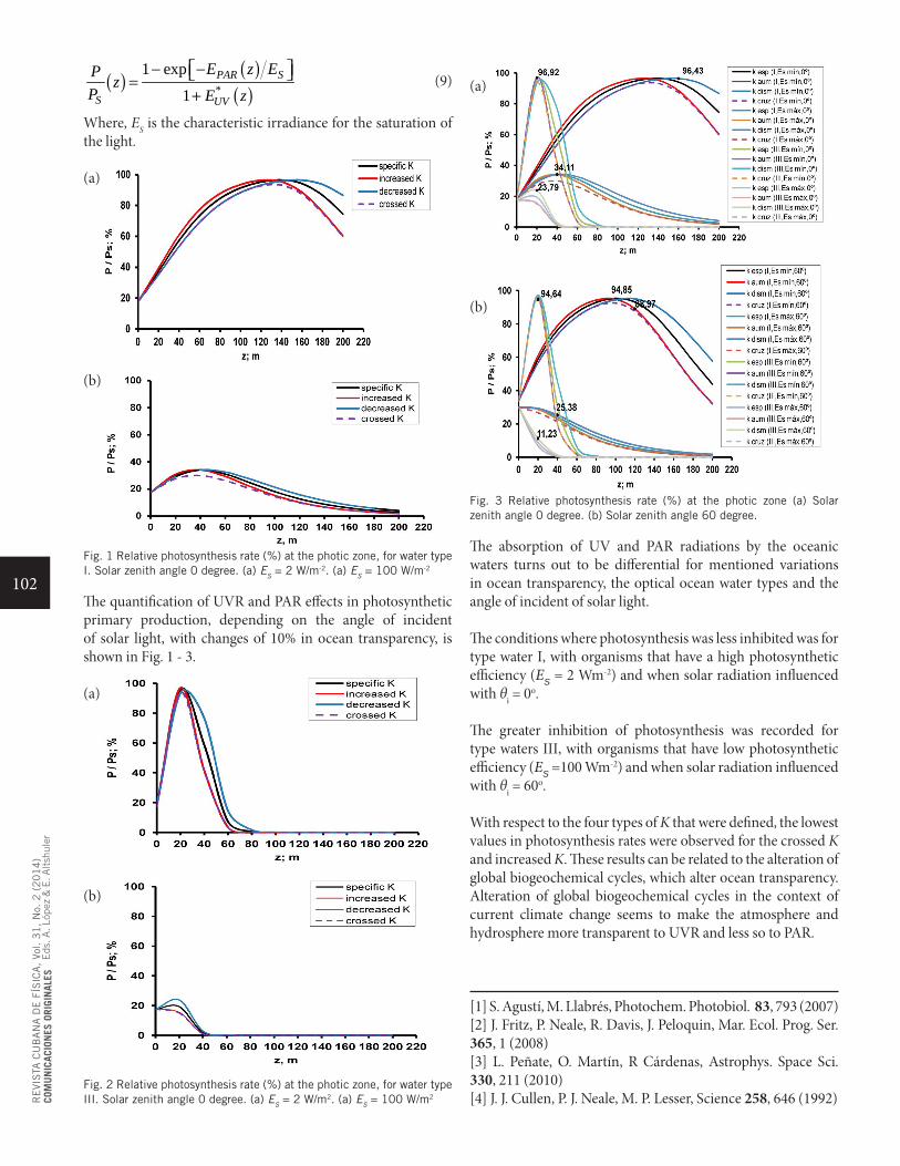
102

RE

VIS

TA C

UB

AN

A D

E F

ÍSIC

A,

Vol. 3

1,

No.

2 (

20

14

)CO

MU

NIC

ACIO

NES

ORI

GIN

ALES

E

ds. A

. Lóp

ez &

E. A

ltsh

uler

( ) ( )( )*

1 exp1

PAR S

S UV

E z EP zP E z

− − =+

(9)

Where, ES is the characteristic irradiance for the saturation of the light.

Fig. 1 Relative photosynthesis rate (%) at the photic zone, for water type I. Solar zenith angle 0 degree. (a) ES = 2 W/m-2. (a) ES = 100 W/m-2

The quantification of UVR and PAR effects in photosynthetic primary production, depending on the angle of incident of solar light, with changes of 10% in ocean transparency, is shown in Fig. 1 - 3.

Fig. 2 Relative photosynthesis rate (%) at the photic zone, for water type III. Solar zenith angle 0 degree. (a) ES = 2 W/m2. (a) ES = 100 W/m2

Fig. 3 Relative photosynthesis rate (%) at the photic zone (a) Solar zenith angle 0 degree. (b) Solar zenith angle 60 degree.

The absorption of UV and PAR radiations by the oceanic waters turns out to be differential for mentioned variations in ocean transparency, the optical ocean water types and the angle of incident of solar light.

The conditions where photosynthesis was less inhibited was for type water I, with organisms that have a high photosynthetic efficiency (ES = 2 Wm-2) and when solar radiation influenced with θi = 0o.

The greater inhibition of photosynthesis was recorded for type waters III, with organisms that have low photosynthetic efficiency (ES =100 Wm-2) and when solar radiation influenced with θi = 60o.

With respect to the four types of K that were defined, the lowest values in photosynthesis rates were observed for the crossed K and increased K. These results can be related to the alteration of global biogeochemical cycles, which alter ocean transparency. Alteration of global biogeochemical cycles in the context of current climate change seems to make the atmosphere and hydrosphere more transparent to UVR and less so to PAR.

[1] S. Agustí, M. Llabrés, Photochem. Photobiol. 83, 793 (2007)[2] J. Fritz, P. Neale, R. Davis, J. Peloquin, Mar. Ecol. Prog. Ser. 365, 1 (2008)[3] L. Peñate, O. Martín, R Cárdenas, Astrophys. Space Sci. 330, 211 (2010)[4] J. J. Cullen, P. J. Neale, M. P. Lesser, Science 258, 646 (1992)

(a)

(b)

(a)

(b)

(a)

(b)

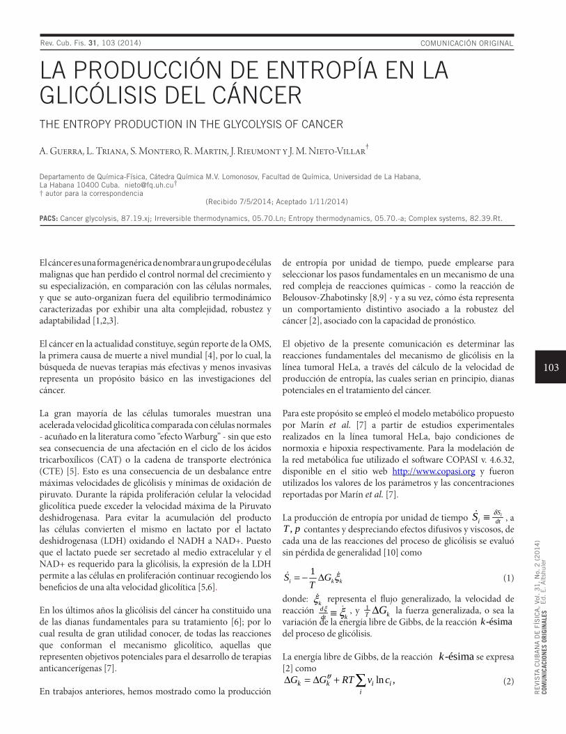
103

RE

VIS

TA C

UB

AN

A D

E F

ÍSIC

A,

Vol. 3

1,

No.

2 (

20

14

)CO

MU

NIC

ACIO

NES

ORI

GIN

ALES

E

d. E

. A

ltsh

uler

COMUNICACIÓN ORIGINAL

LA PRODUCCIÓN DE ENTROPÍA EN LA GLICÓLISIS DEL CÁNCER THE ENTROPY PRODUCTION IN THE GLYCOLYSIS OF CANCER

A. Guerra, L. Triana, S. Montero, R. Martin, J. Rieumont y J. M. Nieto-Villar†

Departamento de Química-Física, Cátedra Química M.V. Lomonosov, Facultad de Química, Universidad de La Habana,La Habana 10400 Cuba. nieto@fq.uh.cu†† autor para la correspondencia

(Recibido 7/5/2014; Aceptado 1/11/2014)

PACS: Cancer glycolysis, 87.19.xj; Irreversible thermodynamics, 05.70.Ln; Entropy thermodynamics, 05.70.-a; Complex systems, 82.39.Rt.

El cáncer es una forma genérica de nombrar a un grupo de células malignas que han perdido el control normal del crecimiento y su especialización, en comparación con las células normales, y que se auto-organizan fuera del equilibrio termodinámico caracterizadas por exhibir una alta complejidad, robustez y adaptabilidad [1,2,3].

El cáncer en la actualidad constituye, según reporte de la OMS, la primera causa de muerte a nivel mundial [4], por lo cual, la búsqueda de nuevas terapias más efectivas y menos invasivas representa un propósito básico en las investigaciones del cáncer.

La gran mayoría de las células tumorales muestran una acelerada velocidad glicolítica comparada con células normales - acuñado en la literatura como “efecto Warburg” - sin que esto sea consecuencia de una afectación en el ciclo de los ácidos tricarboxílicos (CAT) o la cadena de transporte electrónica (CTE) [5]. Esto es una consecuencia de un desbalance entre máximas velocidades de glicólisis y mínimas de oxidación de piruvato. Durante la rápida proliferación celular la velocidad glicolítica puede exceder la velocidad máxima de la Piruvato deshidrogenasa. Para evitar la acumulación del producto las células convierten el mismo en lactato por el lactato deshidrogenasa (LDH) oxidando el NADH a NAD+. Puesto que el lactato puede ser secretado al medio extracelular y el NAD+ es requerido para la glicólisis, la expresión de la LDH permite a las células en proliferación continuar recogiendo los beneficios de una alta velocidad glicolítica [5,6].

En los últimos años la glicólisis del cáncer ha constituido una de las dianas fundamentales para su tratamiento [6]; por lo cual resulta de gran utilidad conocer, de todas las reacciones que conforman el mecanismo glicolítico, aquellas que representen objetivos potenciales para el desarrollo de terapias anticancerígenas [7].

En trabajos anteriores, hemos mostrado como la producción

Rev. Cub. Fis. 31, 103 (2014)

de entropía por unidad de tiempo, puede emplearse para seleccionar los pasos fundamentales en un mecanismo de una red compleja de reacciones químicas - como la reacción de Belousov-Zhabotinsky [8,9] - y a su vez, cómo ésta representa un comportamiento distintivo asociado a la robustez del cáncer [2], asociado con la capacidad de pronóstico.

El objetivo de la presente comunicación es determinar las reacciones fundamentales del mecanismo de glicólisis en la línea tumoral HeLa, a través del cálculo de la velocidad de producción de entropía, las cuales serian en principio, dianas potenciales en el tratamiento del cáncer.

Para este propósito se empleó el modelo metabólico propuesto por Marín et al. [7] a partir de estudios experimentales realizados en la línea tumoral HeLa, bajo condiciones de normoxia e hipoxia respectivamente. Para la modelación de la red metabólica fue utilizado el software COPASI v. 4.6.32, disponible en el sitio web http://www.copasi.org y fueron utilizados los valores de los parámetros y las concentraciones reportadas por Marín et al. [7].

La producción de entropía por unidad de tiempo iSi dtS δ≡ , a

,T p contantes y despreciando efectos difusivos y viscosos, de cada una de las reacciones del proceso de glicólisis se evaluó sin pérdida de generalidad [10] como

1i k kS G

Tξ= − ∆

(1)

donde: kξ representa el flujo generalizado, la velocidad de reacción d

kdtξ ξ≡ , y 1

kT G∆ la fuerza generalizada, o sea la variación de la energía libre de Gibbs, de la reacción -ésimak del proceso de glicólisis.

La energía libre de Gibbs, de la reacción -ésimak se expresa [2] como

ln ,k k i ii

G G RT v cθ∆ = ∆ + ∑

(2)

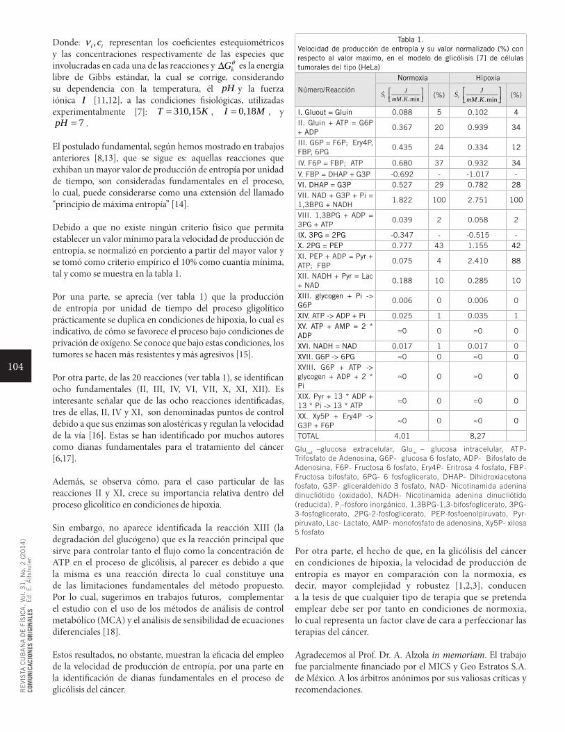
104

RE

VIS

TA C

UB

AN

A D

E F

ÍSIC

A,

Vol. 3

1,

No.

2 (

20

14

)CO

MU

NIC

ACIO

NES

ORI

GIN

ALES

E

d. E

. A

ltsh

uler

Donde: ,i icν representan los coeficientes estequiométricos y las concentraciones respectivamente de las especies que involucradas en cada una de las reacciones y kGθ∆ es la energía libre de Gibbs estándar, la cual se corrige, considerando su dependencia con la temperatura, él pH y la fuerza iónica I [11,12], a las condiciones fisiológicas, utilizadas experimentalmente [7]: 310,15T K= , 0,18I M= , y

7pH = .

El postulado fundamental, según hemos mostrado en trabajos anteriores [8,13], que se sigue es: aquellas reacciones que exhiban un mayor valor de producción de entropía por unidad de tiempo, son consideradas fundamentales en el proceso, lo cual, puede considerarse como una extensión del llamado “principio de máxima entropía” [14].

Debido a que no existe ningún criterio físico que permita establecer un valor mínimo para la velocidad de producción de entropía, se normalizó en porciento a partir del mayor valor y se tomó como criterio empírico el 10% como cuantía mínima, tal y como se muestra en la tabla 1.

Por una parte, se aprecia (ver tabla 1) que la producción de entropía por unidad de tiempo del proceso gligolítico prácticamente se duplica en condiciones de hipoxia, lo cual es indicativo, de cómo se favorece el proceso bajo condiciones de privación de oxígeno. Se conoce que bajo estas condiciones, los tumores se hacen más resistentes y más agresivos [15].

Por otra parte, de las 20 reacciones (ver tabla 1), se identifican ocho fundamentales (II, III, IV, VI, VII, X, XI, XII). Es interesante señalar que de las ocho reacciones identificadas, tres de ellas, II, IV y XI, son denominadas puntos de control debido a que sus enzimas son alostéricas y regulan la velocidad de la vía [16]. Estas se han identificado por muchos autores como dianas fundamentales para el tratamiento del cáncer [6,17].

Además, se observa cómo, para el caso particular de las reacciones II y XI, crece su importancia relativa dentro del proceso glicolítico en condiciones de hipoxia.

Sin embargo, no aparece identificada la reacción XIII (la degradación del glucógeno) que es la reacción principal que sirve para controlar tanto el flujo como la concentración de ATP en el proceso de glicólisis, al parecer es debido a que la misma es una reacción directa lo cual constituye una de las limitaciones fundamentales del método propuesto. Por lo cual, sugerimos en trabajos futuros, complementar el estudio con el uso de los métodos de análisis de control metabólico (MCA) y el análisis de sensibilidad de ecuaciones diferenciales [18].

Estos resultados, no obstante, muestran la eficacia del empleo de la velocidad de producción de entropía, por una parte en la identificación de dianas fundamentales en el proceso de glicólisis del cáncer.

Tabla 1.Velocidad de producción de entropía y su valor normalizado (%) con respecto al valor maximo, en el modelo de glicólisis [7] de células tumorales del tipo (HeLa)

Número/Reacción

Normoxia Hipoxia

. .miniJS

mM K

(%) . .miniJS

mM K

(%)

I. Gluout = Gluin 0.088 5 0.102 4II. Gluin + ATP = G6P + ADP

0.367 20 0.939 34

III. G6P = F6P; Ery4P, FBP, 6PG

0.435 24 0.334 12

IV. F6P = FBP; ATP 0.680 37 0.932 34

V. FBP = DHAP + G3P -0.692 - -1.017 -VI. DHAP = G3P 0.527 29 0.782 28VII. NAD + G3P + Pi = 1,3BPG + NADH

1.822 100 2.751 100

VIII. 1,3BPG + ADP = 3PG + ATP

0.039 2 0.058 2

IX. 3PG = 2PG -0.347 - -0.515 -X. 2PG = PEP 0.777 43 1.155 42XI. PEP + ADP = Pyr + ATP; FBP

0.075 4 2.410 88

XII. NADH + Pyr = Lac + NAD

0.188 10 0.285 10

XIII. glycogen + Pi -> G6P

0.006 0 0.006 0

XIV. ATP -> ADP + Pi 0.025 1 0.035 1XV. ATP + AMP = 2 * ADP

≈0 0 ≈0 0

XVI. NADH = NAD 0.017 1 0.017 0XVII. G6P -> 6PG ≈0 0 ≈0 0XVIII. G6P + ATP -> glycogen + ADP + 2 * Pi

≈0 0 ≈0 0

XIX. Pyr + 13 * ADP + 13 * Pi -> 13 * ATP

≈0 0 ≈0 0

XX. Xy5P + Ery4P -> G3P + F6P

≈0 0 ≈0 0

TOTAL 4,01 8,27

Gluout –glucosa extracelular, Gluin – glucosa intracelular, ATP- Trifosfato de Adenosina, G6P- glucosa 6 fosfato, ADP- Bifosfato de Adenosina, F6P- Fructosa 6 fosfato, Ery4P- Eritrosa 4 fosfato, FBP- Fructosa bifosfato, 6PG- 6 fosfoglicerato, DHAP- Dihidroxiacetona fosfato, G3P- gliceraldehido 3 fosfato, NAD- Nicotinamida adenina dinucliótido (oxidado), NADH- Nicotinamida adenina dinucliótido (reducida), Pi–fósforo inorgánico, 1,3BPG-1,3-bifosfoglicerato, 3PG-3-fosfoglicerato, 2PG-2-fosfoglicerato, PEP-fosfoenolpiruvato, Pyr- piruvato, Lac- Lactato, AMP- monofosfato de adenosina, Xy5P- xilosa 5 fosfato

Por otra parte, el hecho de que, en la glicólisis del cáncer en condiciones de hipoxia, la velocidad de producción de entropía es mayor en comparación con la normoxia, es decir, mayor complejidad y robustez [1,2,3], conducen a la tesis de que cualquier tipo de terapia que se pretenda emplear debe ser por tanto en condiciones de normoxia, lo cual representa un factor clave de cara a perfeccionar las terapias del cáncer.

Agradecemos al Prof. Dr. A. Alzola in memoriam. El trabajo fue parcialmente financiado por el MICS y Geo Estratos S.A. de México. A los árbitros anónimos por sus valiosas críticas y recomendaciones.

105

RE

VIS

TA C

UB

AN

A D

E F

ÍSIC

A,

Vol. 3

1,

No.

2 (

20

14

)CO

MU

NIC

ACIO

NES

ORI

GIN

ALES

E

d. E

. A

ltsh

uler

[1] E. Izquierdo-Kulich & J.M. Nieto-Villar, Chapter 49 "Morphogenesis and Complexity of the Tumor Patterns", R.G. Rubio et al. (eds.), Without Bounds: A Scientific Canvas of Nonlinearity and Complex Dynamics, Understanding Complex Systems, (Springer-Verlag Berlin Heidelberg 2013).[2] E. Izquierdo-Kulich, E. Alonso-Becerra & J.M. Nieto-Villar, J. Modern Physics. 2, 615 (2011).[3] E. Izquierdo-Kulich, I. Rebelo, E. Tejera & J.M. Nieto-Villar, Physica A 392, 6616 (2013).[4] http//: www.oms.org, 2013.[5] Th. N. Seyfried, R. E. Flores, A. M. Poff and D. P. D’Agostino, Carcinogenesis 35, 515 (2014).[6] R. Gatenby & R. Gillies, Int. J. Biochem. Cell B. 39, 1358 (2007).[7] A. Marín, J.C. Gallardo, S. Rodríguez, R. Encalada, R. Moreno, E. Saavedra, Biochim. Biophys. Acta 1807, 755 (2011).[8] J. Rieumont, J.M. Nieto-Villar, J.M. García, An. Quím. 93, 147 (1997).

[9] J.M. Nieto-Villar & M.G. Velarde, J. Non-Equil. Thermody. 25, 269 (2000).[10] G. Nicolis & I. Prigogine, Self-Organization in nonequilibrium systems, (Wiley, New York, 1977).[11] I. Li, R.K. Dash, et al., J. Phys. Chem. B 114, 16068 (2010).[12] R. A. Alberty, Biochemical Thermodynamics: Applications of Mathematica. (Hoboken, Wiley, New York, 2006).[13] J.M. Nieto-Villar, E. Izquierdo-Kulich, R. Quintana y J. Rieumont, Rev. Mex. Fis. 59, 527 (2013).[14] L.M. Martyushev & V.D. Seleznev, Phys. Rep. 264, 1 (2006).[15] S.K. Parks, N.M. Mazure, L. Counillon and J. Pouysségur, J. Cell. Physiol. 228, 1854 (2013).[16] D. L. Nelson & M. Cox Lehninger. Principles of Biochemistry; (5th Edition; W. H. Feeman and Company; New York, 2008).[17] R. B. Hamanaka & N. S. Chandel, Journal Express Medicine 209, 211 (2012).[18] P. A. Iglesias and B. P. Ingalls. Control Theory and Systems Biology; (The MIT Press Cambridge, Massachusetts London, England 2010).

106

RE

VIS

TA C

UB

AN

A D

E F

ÍSIC

A,

Vol. 3

1,

No.

2 (

20

14

)CO

MU

NIC

ACIO

NES

ORI

GIN

ALES

E

ds. A

. C

abo

& E

. A

ltsh

uler

COMUNICACIÓN ORIGINAL

AN ATOMISTIC MODEL OF INTERMOLECULAR INTERACTIONS FOR SIMULATIONS OF LIQUID n-OCTANEMODELO ATOMÍSTICO DE LAS INTERACCIONES INTERMOLECULARES PARA LA SIMULACIÓN DEL LÍQUIDO DE n-OCTANO

B. Rodríguez-Hernández, L. Uranga Piña†, A. Martínez Mesa

Facultad de Física, Universidad de La Habana, Cuba. llinersy@fisica.uh.cu†† corresponding author

(Recibido 22/3/2014 ; Aceptado 22/7/2014)

PACS: Computer simulation of molecular dynamics, 83.10.Rs; Molecular dynamics calculations in liquid structure modeling, 61.20.Ja; Structure of molecular liquids, 61.25.Em

During the last decades, the investigation of dynamical processes at the molecular scale have being largely dominated by the application of Classical Molecular Dynamics (CMD) simulations. In physical and chemical phenomena, classical mechanics often provides an adequate description of underlying nuclear motion, which can be extended up to thousands of atoms and up to the nanosecond or microsecond time-scales [1]. However, an accurate knowledge of the relevant intermolecular interactions is a prerequisite for dynamical calculations, and ab initio electronic structure calculations for relatively large molecular systems continue to pose a tremendous challenge to modern computational physics. As a consequence, assessing the performance of force-fields determined in advance, regarding their ability to reproduce the structural and thermodynamic properties measured in the experiment, is one of the main goals of the molecular dynamics scheme. The united-atom scheme [2–4] leads to a major simplification of the parametrization of the potential energy surface. Within this model, large molecules are replaced by pseudo-atoms located at positions selected according to the symmetry of the molecules.

Simple organic molecules are among the systems for which the application of the united-atom strategy is more interesting, since the representations of intermolecular forces validated for these molecules are expected to be directly transferable to the simulation of the physical properties of a wide range of organic compounds [5–8]. On the other hand, the smallest hydrocarbons are key elements in biological and industrial processes. Moreover, when used as solvents in molecular spectroscopy studies, some substances like n-octane exhibit remarkable properties for which a satisfactory explanation is still lacking. For example, the absorption and fluorescence spectra of some molecules solved in n-octane, present bands whose intensities do not match each other [9]. Due to the

practical importance of these substances, it is highly desirable to count with fairly simple representations of intermolecular forces for the calculation of observables in the liquid phase, without compromising accuracy. In particular, n-octane has many applications in organic synthesis and distillation, and it is one of the fundamental components of gasoline and other oil derivatives.

The purpose of present work is to attain an atomistic description of intermolecular interactions in liquid n-octane, which will be applied to the CMD simulation of this substance. The model introduced here disregards the structure of the molecule, though it is incorporated implicitly in the interaction potential derived from this assumption. The thermodynamics properties of n-octane are evaluated for a wide range of thermodynamic conditions.

We will consider that the microscopic structure of liquid n-octane, as well as its physical properties, can be mimicked by a Lennard-Jones (LJ) fluid with suitable energy, ε, and length, σ, parameters. The Lennard-Jones fluid is defined by the pair potential:

12 6

( ) 4 .LJU rr rσ σε

= −

(1)

Another useful model for liquids consisting in featureless particles is that of the hard sphere (HS) fluid. In this case, the interparticle interaction potential is given by

,( )

0,HSr d

U rr d

∞ <= ≥

(2)

where d is a hard sphere diameter.

Contrary to the Lennard-Jones fluid, the thermodynamic

Rev. Cub. Fis. 31, 106 (2014)

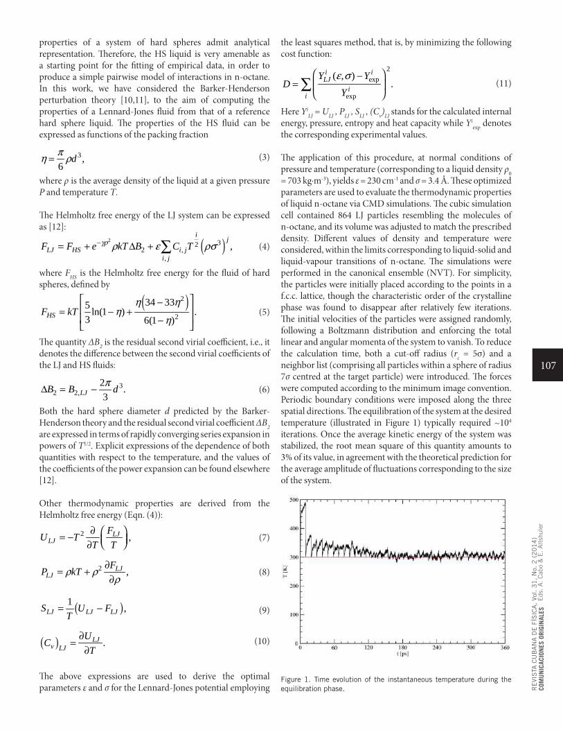
107

RE

VIS

TA C

UB

AN

A D

E F

ÍSIC

A,

Vol. 3

1,

No.

2 (

20

14

)CO

MU

NIC

ACIO

NES

ORI

GIN

ALES

E

ds. A

. C

abo

& E

. A

ltsh

uler

properties of a system of hard spheres admit analytical representation. Therefore, the HS liquid is very amenable as a starting point for the fitting of empirical data, in order to produce a simple pairwise model of interactions in n-octane. In this work, we have considered the Barker-Henderson perturbation theory [10,11], to the aim of computing the properties of a Lennard-Jones fluid from that of a reference hard sphere liquid. The properties of the HS fluid can be expressed as functions of the packing fraction

3,6

dπη ρ=

(3)

where ρ is the average density of the liquid at a given pressure P and temperature T.

The Helmholtz free energy of the LJ system can be expressed as [12]:

( )2 322 ,

,,

ij

LJ HS i ji j

F F e kT B C Tγρ ρ ε ρσ−= + ∆ + ∑

(4)

where FHS is the Helmholtz free energy for the fluid of hard spheres, defined by

( )2

2

34 335 ln(1 ) .3 6(1 )HSF kT

η ηη

η

− = − + −

(5)

The quantity ΔB2 is the residual second virial coefficient, i.e., it denotes the difference between the second virial coefficients of the LJ and HS fluids:

32 2,

2 .3LJB B dπ∆ = −

(6)

Both the hard sphere diameter d predicted by the Barker-Henderson theory and the residual second virial coefficient ΔB2 are expressed in terms of rapidly converging series expansion in powers of T1/2. Explicit expressions of the dependence of both quantities with respect to the temperature, and the values of the coefficients of the power expansion can be found elsewhere [12].

Other thermodynamic properties are derived from the Helmholtz free energy (Eqn. (4)):

2 ,LJLJ

FU T

T T∂ = − ∂

(7)

2 ,LJLJ

FP kTρ ρ

ρ∂

= +∂

(8)

( )1 ,LJ LJ LJS U FT

= −

(9)

( ) .LJv LJ

UC

T∂

=∂

(10)

The above expressions are used to derive the optimal parameters ε and σ for the Lennard-Jones potential employing

the least squares method, that is, by minimizing the following cost function:

2exp

exp

( , ).

i iLJ

ii

Y YD

Y

ε σ −=

∑

(11)

Here YiLJ = ULJ , PLJ , SLJ , (Cv)LJ stands for the calculated internal

energy, pressure, entropy and heat capacity while Yiexp denotes

the corresponding experimental values.

The application of this procedure, at normal conditions of pressure and temperature (corresponding to a liquid density ρ0 = 703 kg·m-3), yields ε = 230 cm-1 and σ = 3.4 Å. These optimized parameters are used to evaluate the thermodynamic properties of liquid n-octane via CMD simulations. The cubic simulation cell contained 864 LJ particles resembling the molecules of n-octane, and its volume was adjusted to match the prescribed density. Different values of density and temperature were considered, within the limits corresponding to liquid-solid and liquid-vapour transitions of n-octane. The simulations were performed in the canonical ensemble (NVT). For simplicity, the particles were initially placed according to the points in a f.c.c. lattice, though the characteristic order of the crystalline phase was found to disappear after relatively few iterations. The initial velocities of the particles were assigned randomly, following a Boltzmann distribution and enforcing the total linear and angular momenta of the system to vanish. To reduce the calculation time, both a cut-off radius (rc = 5σ) and a neighbor list (comprising all particles within a sphere of radius 7σ centred at the target particle) were introduced. The forces were computed according to the minimum image convention. Periodic boundary conditions were imposed along the three spatial directions. The equilibration of the system at the desired temperature (illustrated in Figure 1) typically required ~104 iterations. Once the average kinetic energy of the system was stabilized, the root mean square of this quantity amounts to 3% of its value, in agreement with the theoretical prediction for the average amplitude of fluctuations corresponding to the size of the system.

Figure 1. Time evolution of the instantaneous temperature during the equilibration phase.

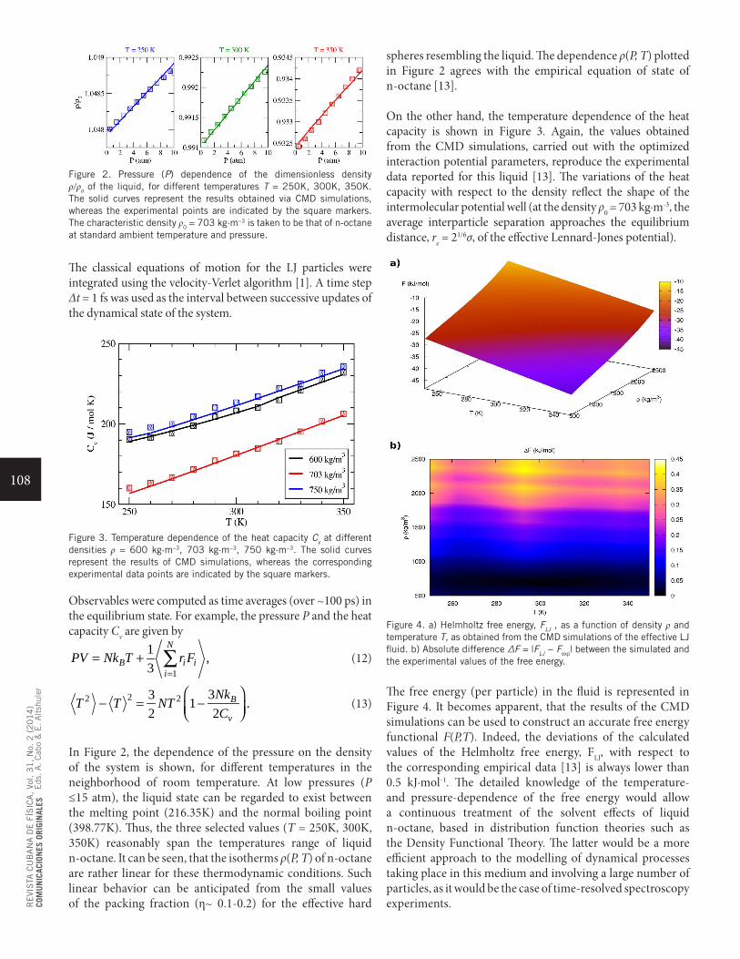
108

RE

VIS

TA C

UB

AN

A D

E F

ÍSIC

A,

Vol. 3

1,

No.

2 (

20

14

)CO

MU

NIC

ACIO

NES

ORI

GIN

ALES

E

ds. A

. C

abo

& E

. A

ltsh

uler

Figure 2. Pressure (P) dependence of the dimensionless density ρ/ρ0 of the liquid, for different temperatures T = 250K, 300K, 350K. The solid curves represent the results obtained via CMD simulations, whereas the experimental points are indicated by the square markers. The characteristic density ρ0 = 703 kg·m−3 is taken to be that of n-octane at standard ambient temperature and pressure.

The classical equations of motion for the LJ particles were integrated using the velocity-Verlet algorithm [1]. A time step Δt = 1 fs was used as the interval between successive updates of the dynamical state of the system.

Figure 3. Temperature dependence of the heat capacity Cv at different densities ρ = 600 kg·m−3, 703 kg·m−3, 750 kg·m−3. The solid curves represent the results of CMD simulations, whereas the corresponding experimental data points are indicated by the square markers.

Observables were computed as time averages (over ~100 ps) in the equilibrium state. For example, the pressure P and the heat capacity Cv are given by

1

1 ,3

N

B i ii

PV Nk T r F=

= + ∑

(12)

22 2 33 1 .2 2

B

v

NkT T NTC

− = −

(13)

In Figure 2, the dependence of the pressure on the density of the system is shown, for different temperatures in the neighborhood of room temperature. At low pressures (P ≤15 atm), the liquid state can be regarded to exist between the melting point (216.35K) and the normal boiling point (398.77K). Thus, the three selected values (T = 250K, 300K, 350K) reasonably span the temperatures range of liquid n-octane. It can be seen, that the isotherms ρ(P, T) of n-octane are rather linear for these thermodynamic conditions. Such linear behavior can be anticipated from the small values of the packing fraction (η~ 0.1-0.2) for the effective hard

spheres resembling the liquid. The dependence ρ(P, T) plotted in Figure 2 agrees with the empirical equation of state of n-octane [13].

On the other hand, the temperature dependence of the heat capacity is shown in Figure 3. Again, the values obtained from the CMD simulations, carried out with the optimized interaction potential parameters, reproduce the experimental data reported for this liquid [13]. The variations of the heat capacity with respect to the density reflect the shape of the intermolecular potential well (at the density ρ0 = 703 kg·m-3, the average interparticle separation approaches the equilibrium distance, re = 21/6σ, of the effective Lennard-Jones potential).

Figure 4. a) Helmholtz free energy, FLJ , as a function of density ρ and temperature T, as obtained from the CMD simulations of the effective LJ fluid. b) Absolute difference ΔF = |FLJ − Fexp| between the simulated and the experimental values of the free energy.

The free energy (per particle) in the fluid is represented in Figure 4. It becomes apparent, that the results of the CMD simulations can be used to construct an accurate free energy functional F(P,T). Indeed, the deviations of the calculated values of the Helmholtz free energy, FLJ, with respect to the corresponding empirical data [13] is always lower than 0.5 kJ·mol-1. The detailed knowledge of the temperature- and pressure-dependence of the free energy would allow a continuous treatment of the solvent effects of liquid n-octane, based in distribution function theories such as the Density Functional Theory. The latter would be a more efficient approach to the modelling of dynamical processes taking place in this medium and involving a large number of particles, as it would be the case of time-resolved spectroscopy experiments.

109

RE

VIS

TA C

UB

AN

A D

E F

ÍSIC

A,

Vol. 3

1,

No.

2 (

20

14

)CO

MU

NIC

ACIO

NES

ORI

GIN

ALES

E

ds. A

. C

abo

& E

. A

ltsh

uler

In this work, we have applied the CMD method to the study of the thermodynamic properties of liquid n-octane, subject to a wide range of conditions of pressure and temperature. The methodology introduced here is based in the Barker-Henderson perturbation theory for a Lennard-Jones fluid. The values obtained for pressure and the heat capacity, are in correspondence with the measurements reported for this system. As an outlook, we plan to incorporate progressively the most important molecular degrees of freedom (rotational,vibrational) to determine a priori the physical properties of liquid n-octane, and to analyze the spectroscopy properties of organic molecules embedded in this medium.

[1] M. P. Allen, D. J. Tildesley, Computer Simulation of Liquids, (Oxford University Press, 1991)[2] J. M. Polson, D. Frenkel, J. Chem. Phys. 111, 1501 (1999)[3] K. Coutinho, M. J. De Oliveira, S. Canuto, Int. J. Quantum

Chem. Symp. 65, 885 (1997)[4] K. Coutinho, S. Canuto, M. C. Zerner, Int. J. Quantum Chem. 66, 249 (1998)[5] A. Lopez Rodriguez, C. Vega, J. J. Freire, J. Chem. Phys. 111, 438 (1999)[6] J. R. Errington, A. Z. Panagiotopoulos, J. Chem. Phys. 111, 9731 (1999)[7] J. Cui, J. R. Elliot Jr., J. Chem. Phys. 116, 8625 (2002)[8] J. Chang, S. I. Sandler, J. Chem. Phys. 121, 7474 (2004)[9] J. S. de Klerk, A. Szemik-Hojniak, F. Ariese, C. Gooijer, J. Phys. Chem. A 111, 5828 (2007)[10] J. P. Hansen, I. R. McDonald, Theory of simple liquids, (Academic Press, 1986)[11] B.-J. Zhang, Fluid Phase Equil. 154, 1 (1999)[12] J. Kolafa, I. Nezbeda, Fluid Phase Equil. 100, 1 (1994)[13] E. W. Lemmon, M. O. McLinden, D. G. Friend, “Thermophysical Properties of Fluid Systems” in NIST Chem-istry WebBook, NIST Standard Reference Database Number 69, Eds. P.J. Linstrom and W.G. Mallard, National Institute of Standards and Technology, Gaithersburg MD, 20899, http://webbook.nist.gov

110

RE

VIS

TA C

UB

AN

A D

E F

ÍSIC

A,

Vol. 3

1,

No.

2 (

20

14

)CO

MU

NIC

ACIO

NES

ORI

GIN

ALES

E

ds. A

. C

abo

& E

. A

ltsh

uler

COMUNICACIÓN ORIGINAL

MOLECULAR DYNAMICSIN HYPERSPHERICAL COORDINATESDINÁMICA MOLECULAR EN COORDENADAS HIPERESFÉRICAS

V. M. Freixas Lemus, A. Martínez Mesa and L. Uranga Piña†

Facultad de Física, Universidad de La Habana, Cuba. llinersy@fisica.uh.cu†† corresponding author

(Recibido 25/3/2014 ; Aceptado 22/7/2014)

PACS: Hyperspherical methods (atomic physics), 31.15.xj; Scattering in atomic and molecular collisions, 34.80.-i; Molecular dynamics calculations in atomic and molecular physics, 31.15.xv

The remarkable progress experienced during the last decade by the set of experimental techniques known as femtosecond spectroscopy, has significantly stimulated the investigation of dynamical processes at the molecular scale, especially via computer simulations. Ultrafast spectroscopy experiments provide direct information on the evolution of molecular phenomena in the femtosecond time-scale. On the other hand, theoretical studies allow to translate the experimental information into an explicit representation of atomic motion. These data may be used to design control strategies to manipulate the dynamics of the molecular systems in order to optimize, for instance, the formation of a target molecule. Computer simulations exhibit some additional advantages, such as the possibility to address the calculation of observables that can not be accessed empirically. It is also useful to carry out an artificial separation of the different components of the intermolecular interactions (e.g., the isotropically averaged potential, anisotropic contributions, local minima, etc.), and to evaluate the influence of each one of these contributions on the calculated observables.

Reactive collisions, i.e., those where bond breaking and formation occur, constitute examples of dynamical processes that can not be treated properly within the standard scattering theory. For example, for triatomic systems, the change in the bonding character enforces it to be treated explicitly as a three-body problem. Because of the rapid increase of the computational resources necessary to undertake the simulations of a molecular system as its size becomes larger, it is very important to find a representation of the molecular motion that enables the solution of the resulting equations of motion to be handled efficiently.

The purpose of this paper is to discuss the advantages of hyperspherical coordinates for the study of molecular dynamics, with emphasis on the case of triatomic systems. Hyperspherical coordinates constitute alternative representations of the molecular motion [1-6]. These

generalized coordinates transform the problem of n particles moving in a D-dimensional space, after the elimination of the motion of the centre of mass, into that of a single particle of mass / ( )a b c a b cm m m m m mµ = + + that moves in a d-dimensional hypersphere (d=(n−1)D) whose variable (hyper)radius is ρ. The position on the hypersurface is specified by d−1 hyperangles.

There are many different angular parametrizations, such as the asymmetric (or Fock), symmetric (or Smith) and Johnson coordinates [3]. The freedom to choose the parametrization which is better suited for every possible application is one of the more appealing features the method. The majority of the investigations carried out so far in the hyperspherical framework are based on the time-independent scattering theory. Therefore, the unique perspective emerging from the time-dependent approach to quantum dynamics has remained practically unexplored. The study of the time evolution of reactive collisions in the hyperspherical formalism to be addressed here, is performed by means of the Classical Molecular Dynamics method. As it will be explained bellow, the deviations arising from neglecting quantum effects are alleviated by the particular choice of the potential energy surface.

As a numerical example, we will focus our attention in the F + HCl → FH + Cl exchange reaction. Owing to the availability of experimental and theoretical results, this kind of reactive collisions constitute an ideal benchmark to test novel algorithms, for which an application to the numerical simulation of dynamical processes of molecular systems in the gas phase is envisaged. From the practical point of view, this reaction also has potential applications in the design and fabrication of chemical lasers [8,9].

Jacobi vectors are the most widely used set of dynamical variables to specify the configuration of polyatomic systems. This preference is due to the simplicity of the classical and the

Rev. Cub. Fis. 31, 110 (2014)

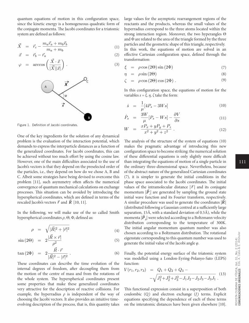
111

RE

VIS

TA C

UB

AN

A D

E F

ÍSIC

A,

Vol. 3

1,

No.

2 (

20

14

)CO

MU

NIC

ACIO

NES

ORI

GIN

ALES

E

ds. A

. C

abo

& E

. A

ltsh

uler

quantum equations of motion in this configuration space, since the kinetic energy is a homogeneous quadratic form of the conjugate momenta. The Jacobi coordinates for a triatomic system are defined as follows:

X = rc −mara +mbrbma +mb

x = rb − ra

ϕ = arccos

( X · x| X||x|

).

(3)

Figure 1. Definition of Jacobi coordinates.

One of the key ingredients for the solution of any dynamical problem is the evaluation of the interaction potential, which demands to express the interparticle distances as a function of the generalized coordinates. For Jacobi coordinates, this can be achieved without too much effort by using the cosine law. However, one of the main difficulties associated to the use of Jacobi’s vectors is that they depend on the preselected order of the particles, i.e., they depend on how do we chose A, B and C. Albeit some strategies have being devised to overcome this problem [11], such asymmetry often affects the numerical convergence of quantum mechanical calculations on exchange processes. This situation can be avoided by introducing the hyperspherical coordinates, which are defined in terms of the rescaled Jacobi’s vectors r and R

[10, 11].

In the following, we will make use of the so called Smith hyperspherical coordinates ρ, Θ, Φ, defined as:

ρ =

√|R|2 + |r|2

sin (2Θ) = 2|R× r|

ρ2

tan (2Φ) = 2R · r

|R|2 − |r|2.

(6)

These coordinates can describe the time evolution of the internal degrees of freedom, after decoupling them from the motion of the centre of mass and from the rotations of the whole system. The hyperspherical coordinates present some properties that make these generalized coordinates very attractive for the description of reactive collisions. For example, the hyperradius ρ is independent of the way of choosing the Jacobi vectors. It also provides an intuitive time-evolving description of the process, that is, this quantity takes

(1)

(2)

(5)

(4)

large values for the asymptotic rearrangement regions of the reactants and the products, whereas the small values of the hyperradius correspond to the three atoms located within the strong interaction region. Moreover, the two hyperangles Θ and Φ are related to the area of the triangle formed by the three particles and the geometric shape of this triangle, respectively. In this work, the equations of motion are solved in an effective Cartesian configuration space, defined through the transformation:

ξ = ρ cos (2Θ) sin (2Φ)

η = ρ sin (2Θ)

ζ = ρ cos (2Θ) cos (2Φ) . (9)

In this configuration space, the equations of motion for the variables s = ξ, η, ζ take the form:

s =1

µ[4Ps − 3Ws]

Ps =3W

µ[Ps −Ws]− ∂V

∂s

W =xPx + yPy + Pz

x2 + y2 + z2. (12)

The analysis of the structure of the system of equations (10) makes the pragmatic advantage of introducing this new configuration space to become striking: the numerical solution of these differential equations is only slightly more difficult than integrating the equations of motion of a single particle in the ordinary three-dimensional space. Nevertheless, because of the abstract nature of the generalized Cartesian coordinates (7), it is simpler to generate the initial conditions in the phase space associated to the Jacobi coordinates. The initial values of the intramolecular distance | r | and its conjugate momentum |P

r| are generated by sampling the ground state initial wave function and its Fourier transform, respectively. A similar procedure was used to generate the coordinates |R

| (distributed following a Gaussian centred at a sufficiently large separation, 15Å, with a standard deviation of 0.5Å), while the momenta |P

R| were selected according to a Boltzmann velocity distribution corresponding to the temperature of 300K. The initial angular momentum quantum number was also chosen according to a Boltzmann distribution. The rotational eigenstate corresponding to this quantum number was used to generate the initial value of the Jacobi angle φ.

Finally, the potential energy surface of the triatomic system was modelled using a London-Eyring-Polanyo-Sato (LEPS) function: V (r1, r2, r3) = Q1 +Q2 +Q3 −

−√J21+J2

2+J23−J1J2−J2J3−J3J1 .

(13)

This functional expression consist in a superposition of both coulombic (Qi) and electron exchange (Ji) terms. Explicit equations specifying the dependence of each of these terms on the interatomic distances have been given elsewhere [10].

(7)(8)

(11)

(10)

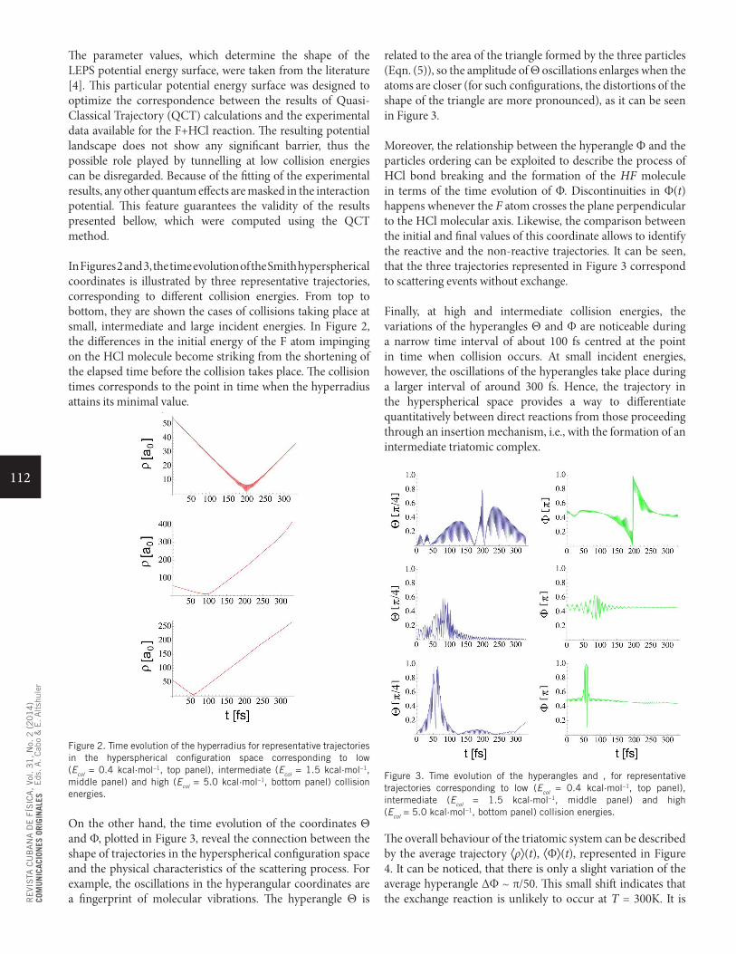
112

RE

VIS

TA C

UB

AN

A D

E F

ÍSIC

A,

Vol. 3

1,

No.

2 (

20

14

)CO

MU

NIC

ACIO

NES

ORI

GIN

ALES

E

ds. A

. C

abo

& E

. A

ltsh

uler

The parameter values, which determine the shape of the LEPS potential energy surface, were taken from the literature [4]. This particular potential energy surface was designed to optimize the correspondence between the results of Quasi-Classical Trajectory (QCT) calculations and the experimental data available for the F+HCl reaction. The resulting potential landscape does not show any significant barrier, thus the possible role played by tunnelling at low collision energies can be disregarded. Because of the fitting of the experimental results, any other quantum effects are masked in the interaction potential. This feature guarantees the validity of the results presented bellow, which were computed using the QCT method.

In Figures 2 and 3, the time evolution of the Smith hyperspherical coordinates is illustrated by three representative trajectories, corresponding to different collision energies. From top to bottom, they are shown the cases of collisions taking place at small, intermediate and large incident energies. In Figure 2, the differences in the initial energy of the F atom impinging on the HCl molecule become striking from the shortening of the elapsed time before the collision takes place. The collision times corresponds to the point in time when the hyperradius attains its minimal value.

Figure 2. Time evolution of the hyperradius for representative trajectories in the hyperspherical configuration space corresponding to low (Ecol = 0.4 kcal·mol−1, top panel), intermediate (Ecol = 1.5 kcal·mol−1, middle panel) and high (Ecol = 5.0 kcal·mol−1, bottom panel) collision energies.

On the other hand, the time evolution of the coordinates Θ and Φ, plotted in Figure 3, reveal the connection between the shape of trajectories in the hyperspherical configuration space and the physical characteristics of the scattering process. For example, the oscillations in the hyperangular coordinates are a fingerprint of molecular vibrations. The hyperangle Θ is

related to the area of the triangle formed by the three particles (Eqn. (5)), so the amplitude of Θ oscillations enlarges when the atoms are closer (for such configurations, the distortions of the shape of the triangle are more pronounced), as it can be seen in Figure 3.

Moreover, the relationship between the hyperangle Φ and the particles ordering can be exploited to describe the process of HCl bond breaking and the formation of the HF molecule in terms of the time evolution of Φ. Discontinuities in Φ(t) happens whenever the F atom crosses the plane perpendicular to the HCl molecular axis. Likewise, the comparison between the initial and final values of this coordinate allows to identify the reactive and the non-reactive trajectories. It can be seen, that the three trajectories represented in Figure 3 correspond to scattering events without exchange.

Finally, at high and intermediate collision energies, the variations of the hyperangles Θ and Φ are noticeable during a narrow time interval of about 100 fs centred at the point in time when collision occurs. At small incident energies, however, the oscillations of the hyperangles take place during a larger interval of around 300 fs. Hence, the trajectory in the hyperspherical space provides a way to differentiate quantitatively between direct reactions from those proceeding through an insertion mechanism, i.e., with the formation of an intermediate triatomic complex.

Figure 3. Time evolution of the hyperangles and , for representative trajectories corresponding to low (Ecol = 0.4 kcal·mol−1, top panel), intermediate (Ecol = 1.5 kcal·mol−1, middle panel) and high (Ecol = 5.0 kcal·mol−1, bottom panel) collision energies.

The overall behaviour of the triatomic system can be described by the average trajectory ⟨ρ⟩(t), ⟨Φ⟩(t), represented in Figure 4. It can be noticed, that there is only a slight variation of the average hyperangle ΔΦ ~ π/50. This small shift indicates that the exchange reaction is unlikely to occur at T = 300K. It is

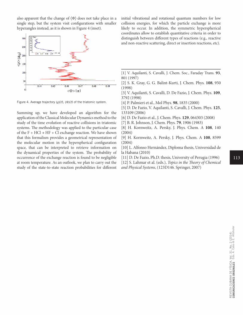
113

RE

VIS

TA C

UB

AN

A D

E F

ÍSIC

A,

Vol. 3

1,

No.

2 (

20

14

)CO

MU

NIC

ACIO

NES

ORI

GIN

ALES

E

ds. A

. C

abo

& E

. A

ltsh

uler

also apparent that the change of ⟨Φ⟩ does not take place in a single step, but the system visit configurations with smaller hyperangles instead, as it is shown in Figure 4 (inset).

Figure 4. Average trajectory ⟨ϱ⟩(t), ⟨Φ⟩(t) of the triatomic system.

Summing up, we have developed an algorithm for the application of the Classical Molecular Dynamics method to the study of the time evolution of reactive collisions in triatomic systems. The methodology was applied to the particular case of the F + HCl → HF + Cl exchange reaction. We have shown that this formalism provides a geometrical representation of the molecular motion in the hyperspherical configuration space, that can be interpreted to retrieve information on the dynamical properties of the system. The probability of occurrence of the exchange reaction is found to be negligible at room temperature. As an outlook, we plan to carry out the study of the state-to-state reaction probabilities for different

initial vibrational and rotational quantum numbers for low collision energies, for which the particle exchange is more likely to occur. In addition, the symmetric hyperspherical coordinates allow to establish quantitative criteria in order to distinguish between different types of reactions (e.g., reactive and non-reactive scattering, direct or insertion reactions, etc).

[1] V. Aquilanti, S. Cavalli, J. Chem. Soc., Faraday Trans. 93, 801 (1997)[2] S. K. Gray, G. G. Balint-Kurti, J. Chem. Phys. 108, 950 (1998)[3] V. Aquilanti, S. Cavalli, D. De Fazio, J. Chem. Phys. 109, 3792 (1998)[4] P. Palmieri et al., Mol Phys. 98, 1835 (2000)[5] D. De Fazio, V. Aquilanti, S. Cavalli, J. Chem. Phys. 125, 133109 (2006)[6] D. De Fazio et al., J. Chem. Phys. 129, 064303 (2008)[7] B. R. Johnson, J. Chem. Phys. 79, 1906 (1983)[8] H. Kornweitz, A. Persky, J. Phys. Chem. A 108, 140 (2004)[9] H. Kornweitz, A. Persky, J. Phys. Chem. A 108, 8599 (2004)[10] L. Alfonso Hernández, Diploma thesis, Universidad de la Habana (2010)[11] D. De Fazio, Ph.D. thesis, University of Perugia (1996)[12] S. Lahmar et al. (eds.), Topics in the Theory of Chemical and Physical Systems, (123D146. Springer, 2007)

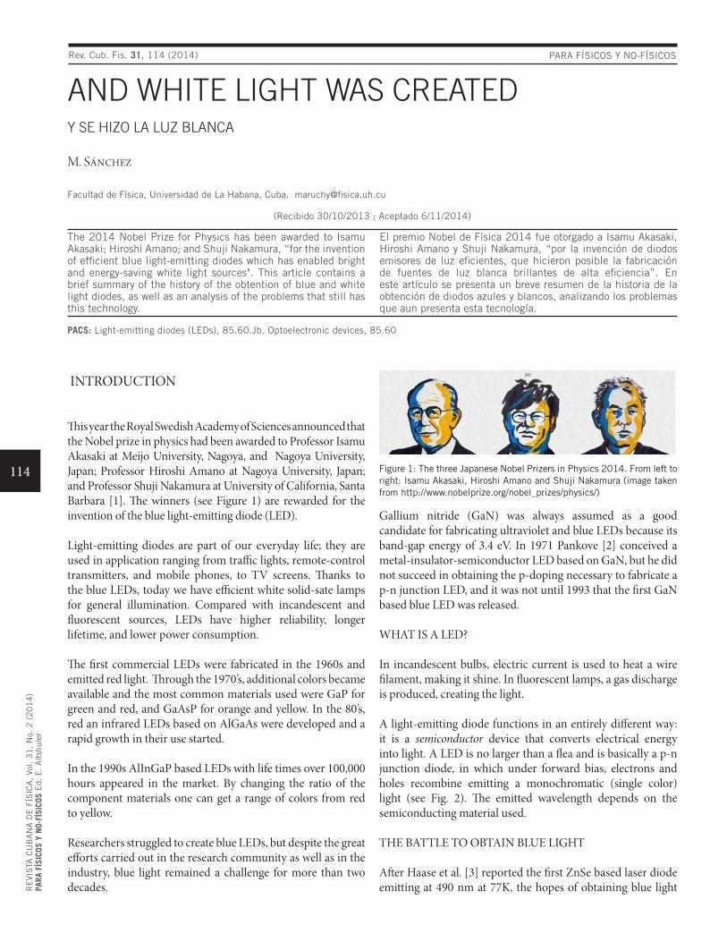
114

RE

VIS

TA C

UB

AN

A D

E F

ÍSIC

A,

Vol. 3

1,

No.

2 (

20

14

)PA

RA F

ÍSIC

OS Y

NO-

FÍSI

COS

Ed.

E. A

ltsh

uler

PARA FÍSICOS Y NO-FÍSICOS

AND WHITE LIGHT WAS CREATED Y SE HIZO LA LUZ BLANCA

M. Sánchez

Facultad de Física, Universidad de La Habana, Cuba. maruchy@fisica.uh.cu

(Recibido 30/10/2013 ; Aceptado 6/11/2014)

The 2014 Nobel Prize for Physics has been awarded to Isamu Akasaki; Hiroshi Amano; and Shuji Nakamura, “for the invention of efficient blue light-emitting diodes which has enabled bright and energy-saving white light sources". This article contains a brief summary of the history of the obtention of blue and white light diodes, as well as an analysis of the problems that still has this technology.

El premio Nobel de Física 2014 fue otorgado a Isamu Akasaki, Hiroshi Amano y Shuji Nakamura, “por la invención de diodos emisores de luz eficientes, que hicieron posible la fabricación de fuentes de luz blanca brillantes de alta eficiencia”. En este artículo se presenta un breve resumen de la historia de la obtención de diodos azules y blancos, analizando los problemas que aun presenta esta tecnología.

PACS: Light-emitting diodes (LEDs), 85.60.Jb. Optoelectronic devices, 85.60

INTRODUCTION

This year the Royal Swedish Academy of Sciences announced that the Nobel prize in physics had been awarded to Professor Isamu Akasaki at Meijo University, Nagoya, and Nagoya University, Japan; Professor Hiroshi Amano at Nagoya University, Japan; and Professor Shuji Nakamura at University of California, Santa Barbara [1]. The winners (see Figure 1) are rewarded for the invention of the blue light-emitting diode (LED).

Light-emitting diodes are part of our everyday life; they are used in application ranging from traffic lights, remote-control transmitters, and mobile phones, to TV screens. Thanks to the blue LEDs, today we have efficient white solid-sate lamps for general illumination. Compared with incandescent and fluorescent sources, LEDs have higher reliability, longer lifetime, and lower power consumption.

The first commercial LEDs were fabricated in the 1960s and emitted red light. Through the 1970’s, additional colors became available and the most common materials used were GaP for green and red, and GaAsP for orange and yellow. In the 80’s, red an infrared LEDs based on AlGaAs were developed and a rapid growth in their use started.

In the 1990s AlInGaP based LEDs with life times over 100,000 hours appeared in the market. By changing the ratio of the component materials one can get a range of colors from red to yellow.

Researchers struggled to create blue LEDs, but despite the great efforts carried out in the research community as well as in the industry, blue light remained a challenge for more than two decades.

Figure 1: The three Japanese Nobel Prizers in Physics 2014. From left to right: Isamu Akasaki, Hiroshi Amano and Shuji Nakamura (image taken from http://www.nobelprize.org/nobel_prizes/physics/)

Gallium nitride (GaN) was always assumed as a good candidate for fabricating ultraviolet and blue LEDs because its band-gap energy of 3.4 eV. In 1971 Pankove [2] conceived a metal-insulator-semiconductor LED based on GaN, but he did not succeed in obtaining the p-doping necessary to fabricate a p-n junction LED, and it was not until 1993 that the first GaN based blue LED was released.

WHAT IS A LED?

In incandescent bulbs, electric current is used to heat a wire filament, making it shine. In fluorescent lamps, a gas discharge is produced, creating the light.

A light-emitting diode functions in an entirely different way: it is a semiconductor device that converts electrical energy into light. A LED is no larger than a flea and is basically a p-n junction diode, in which under forward bias, electrons and holes recombine emitting a monochromatic (single color) light (see Fig. 2). The emitted wavelength depends on the semiconducting material used.

THE BATTLE TO OBTAIN BLUE LIGHT

After Haase et al. [3] reported the first ZnSe based laser diode emitting at 490 nm at 77K, the hopes of obtaining blue light

Rev. Cub. Fis. 31, 114 (2014)

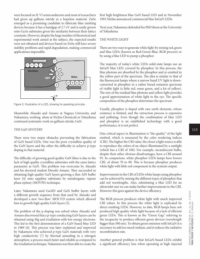
115

RE

VIS

TA C

UB

AN

A D

E F

ÍSIC

A,

Vol. 3

1,

No.

2 (

20

14

)PA

RA F

ÍSIC

OS Y

NO-

FÍSI

COS

Ed.

E. A

ltsh

uler

were focused on II-VI semiconductors and most of researchers had given up gallium nitride as a hopeless material. ZnSe emerged as a promising candidate to fabricate blue emitting devices because it has a bandgap of 2.7 eV and is easily grown onto GaAs substrates given the similarity between their lattice constants. However, despite the large number of theoretical and experimental work aimed at the subject, the expected results were not obtained and devices based on ZnSe still have severe stability problems and rapid degradation, making commercial applications impossible.

Figure 2: Illustration of a LED, showing its operating principle.

Meanwhile Akasaki and Amano at Nagoya University, and Nakamura, working alone at Nichia Chemicals in Tokushima continued systematic work on gallium nitride, GaN.

THE GaN MYSTERY

There were two major obstacles preventing the fabrication of GaN based LEDs. One was the poor crystalline quality of the GaN layers and the other the difficulty to achieve p-type doping in that material.

The difficulty of growing good quality GaN films is due to the lack of high quality crystalline substrates with the same lattice parameter as GaN. This problem was overcome by Akasaki and his doctoral student Hiroshi Amano. They succeeded in obtaining high-quality GaN layers growing a thin AlN buffer layer [4] onto sapphire substrates by metalorganic vapour phase epitaxy (MOVPE) technique.

Later, Nakamura used GaAlN and GaN buffer layers with a different growth sequence from that used by Akasaki and developed a new ‘two-flow’ MOCVD system which allowed him to growth high quality GaN layers [5].

The problem of the p-doping was solved when Akasaki and Amano discovered that a p-type conducting GaN layers can be obtained using Mg and irradiation with low energy electrons. This led to the first demonstration of a GaN based blue LED in 1989 [6]. This process was later explained and improved by Nakamura who achieved p-type GaN materials with very high conductivity [7] by thermal annealing in a nitrogen atmosphere, a process much faster and reliable as compared to the irradiation technique. Nakamura was then able to create the

first high-brightness blue GaN based LED and in November 1993 Nichia announced commercial blue InGaN LEDs.

Next year, Nakamura defended his PhD thesis at the University of Tokushima

THE WHITE LIGHT

There are two ways to generate white light: by mixing red, green and blue LEDs (known as Red-Green-Blue, RGB process) or by using a blue LED to pump a phosphor.

The majority of today’s white LEDs solid-state lamps use an InGaN blue LED, covered by phosphor. In this process, the blue photons are absorbed by the phosphor and re-emitted in the yellow part of the spectrum. The idea is similar to that of the fluorescent lamps where a narrow band UV light is down-converted in phosphor to a rather broad emission spectrum of visible light (a little red, some green, and a lot of yellow). The mix of the residual blue photons and yellow light provides a good approximation of white light to the eye. The specific composition of the phosphor determines the spectrum.

Usually, phosphor is doped with rare earth elements, whose existence is limited, and the extraction process is expensive and polluting. Even though the combination of blue LED and phosphor is an established technology with a good performance, it is not perfect.

One critical aspect in illumination is “the quality” of the light emitted, which is measured by the color rendering indices (CRI). The higher the CRI value, the closer a light source is able to reproduce the colors of an object illuminated by a sunlight (which has a CRI of 100). For example, incandescent bulbs, despite their other obvious disadvantages, have a CRI around 95. In comparison, white phosphor LEDs lamps have lowers CRI, of about 70 to 80. This is because phosphor produces white light with little red component in the system’s output.

Improvements in the CRI of LEDs white lamps using phosphor can be achieved by mixing the different types of phosphor that add red wavelengths. Also, substituting a blue LED for an ultraviolet one we can make further improvements to the CRI. However this goes against the device efficiency.

The RGB process produces white light with much improved CRI values. In this process the white light is replicated by direct emitting LEDs. However, to date, RGB lamps have not produced high quality white light because of a lack of efficient green LEDs. This is known as the “Green Gap,” referring to the incapacity to produce efficient green devices (wavelength bigger than 500 nm). To obtain green emission with InGaN it is necessary to add too much indium, and it reduces the radiative recombination rate.

Another general problem is that InGaN-based LEDs exhibit a significant efficiency loss when operating at high injected

116

RE

VIS

TA C

UB

AN

A D

E F

ÍSIC

A,

Vol. 3

1,

No.

2 (

20

14

)PA

RA F

ÍSIC

OS Y

NO-

FÍSI

COS

Ed.

E. A

ltsh

uler

current densities, the origin of which remains as an open issue [8].

Despite these problems Cree announced this year a white high-power LED with 300 lumens per watt, which increases the potential for the solid-state-lighting industry.

InGaN LASERS

Not only the fabrication of blue LEDs has had a huge technological impact: the creation of blue lasers diodes (LDs) has been of great importance too. For example, the storage density in digital video disks (DVDs) is bigger for shorter wavelengths of the laser used to write and read the information, since the focused light diameter decreases (more precisely, the storage density is inversely proportional to the square of the wavelength). So, blue-based InGaN lasers allow to increases the data-storage density in modern digital video disks (DVDs). Previous DVDs, used red AlInGaP semiconductor lasers and had a data capacity of about 4.7 gigabytes.

The first nitride based violet LDs with an emission wavelength of around 400 nm at room temperature were developed by Nakamura in 1996 [9]. Finally, in January 1999 the first commercial violet laser entered the market. More details can be found in ref. [10].

A FINAL REMARK

As has been said, Alfred Nobel would have been quite pleased with the 2015 Physics prize. The invention of the blue LED

means a great benefit to mankind, and there are good reasons to think that we are just contemplating the tip of the iceberg. That is definitively in the spirit of Nobel’s legacy.

[1] The Nobel Prize in Physics 2014 - Nobelprize.org. http://www.nobelprize.org/nobel_prizes/physics/laureates/2014/[2] J. I Pankove, E. A. Miller and J. E. Berkeyheiser, RCA Rev. 32, 383 (1971).[3] M. A. Hasse, J. Qiu, J. M. De Puydt and H. Cheng, Appl. Phys. Lett. 59, 1272 (1991).[4] H. Amano et al., Appl. Phys. Lett. 48, 353 (1986).[5] S. Nakamura and T. Mukai, Jpn. .J. Appl. Physics 31, L1457 (1992).[6] I. Akasaki, H. Amano, Y. Koide, K. Hiramatsy and N. Sawaki, J. Crvst. Growth 98, 209 (1989).[7] S. Nakamura, N. Iwasa, M. Senoh and T. Mukai, Jpn. J. Appl. Phys., 31, 1258. (1992).[8] G. Verzellesi, D. Saguatti, M. Meneghini, F. Bertazzi, M. Goano, G. Meneghesso and E. Zanoni. J. Appl. Phys. 114, 071101 (2013).[9] S. Nakamura, M. Senoh, S. Nagahama, N. Iwasa, T. Yamada, T. Matsushita, H. Kiyoku and Y. Sugimoto, Jpn. J. Appl. Phys. 35, L74 (1996). [10] S. Nakamura, S. Pearton, G. Fasol. The Blue laser Diode. 2nd Ed. (Springer-Verlag Berlin Heidelberg, 2000)

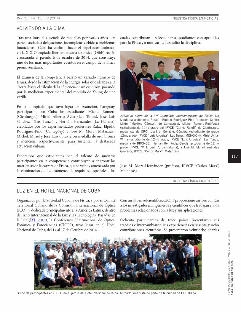
117

RE

VIS

TA C

UB

AN

A D

E F

ÍSIC

A,

Vol. 3

1,

No.

2 (

20

14

)N

UES

TRA

FÍSI

CA E

N N

OTIC

IAS

NUESTRA FÍSICA EN NOTICIASRev. Cub. Fis. 31, 117 (2014)

VOLVIENDO A LA CIMA

Tras una inusual ausencia de medallas por varios años –en parte asociada a delegaciones incompletas debido a problemas financieros– Cuba ha vuelto a hacer el papel acostumbrado en la XIX Olimpiada Iberoamericana de Física (OibF) recién clausurada el pasado 6 de octubre de 2014, que constituye uno de los más importantes eventos en el campo de la Física preuniversitaria.

El examen de la competencia barrió un variado número de temas: desde la estimación de la energía solar que alcanza a la Tierra, hasta el cálculo de la eficiencia de un ciclotrón, pasando por la medición experimental del módulo de Young de una varilla.

En la olimpiada, que tuvo lugar en Asunción, Paraguay, participaron por Cuba los estudiantes Michel Romero (Cienfuegos), Miriel Alberto Ávila (Las Tunas), José Luis Sánchez (Las Tunas) y Hernán Hernández (La Habana), escoltados por los experimentados profesores Rafael Elpidio Rodríguez-Pino (Camagüey) y José M. Mora (Matanzas). Michel, Miriel y José Luis obtuvieron medalla de oro, bronce y mención, respectivamente, para sustentar la destacada actuación cubana.

Esperamos que estudiantes con el talento de nuestros participantes en la competencia contribuyan a engrosar las matrículas de la carrera de Física, que se ve hoy amenazada por la eliminación de los exámenes de requisitos especiales –los

cuales contribuían a seleccionar a estudiantes con aptitudes para la Física y a motivarlos a estudiar la disciplina.

Júbilo al cierre de la XIX Olimpíada Iberoamericana de Física. De izquierda a derecha: Rafael Elpidio Rodríguez-Pino (profesor, Centro Mixto “Máximo Gómez”, de Camagüey), Michel Romero-Rodríguez (estudiante de 11no grado del IPVCE “Carlos Roloff” de Cienfuegos, medallista de ORO), José L. González-Góngora (estudiante de grado 12mo grado, IPVCE “Luis Urquiza”, Las Tunas, MENCIÓN), Miriel Ávila-Winta (estudiante de 12mo grado, IPVCE “Luis Urquiza”, Las Tunas, medalla de BRONCE), Hernán Hernández-García (estudiante de 12mo grado, IPVCE “V. I. Lenin”, La Habana), y José M. Mora-Hernández (profesor, IPVCE “Carlos Marx”, Matanzas).

José M. Mora-Hernández (profesor, IPVCE “Carlos Marx”, Matanzas).

NUESTRA FÍSICA EN NOTICIAS

LUZ EN EL HOTEL NACIONAL DE CUBA

Organizada por la Sociedad Cubana de Física, y por el Comité Territorial Cubano de la Comisión Internacional de Óptica (ICO), y dedicada principalmente a la América Latina, dentro del Año Internacional de la Luz y las Tecnologías Basadas en la Luz (IYL 2015), la Conferencia Internacional de Óptica, Fotónica y Fotociencias (CIOFF), tuvo lugar en el Hotel Nacional de Cuba, del 14 al 17 de Octubre de 2014.

Con un alto nivel científico, CIOFF proporcionó un foro común a los investigadores, ingenieros y científicos que trabajan en los problemas relacionados con la luz y sus aplicaciones.

Ochenta participantes de trece países presentaron sus trabajos e intercambiaron sus experiencias en sesenta y ocho contribuciones científicas. Se presentaron veintiocho charlas

Grupo de participantes en CIOFF, en el jardín del Hotel Nacional de Cuba. Al fondo, una vista de parte de la ciudad de La Habana.

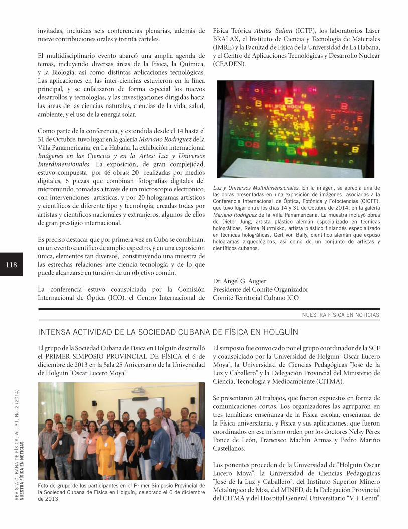
118

RE

VIS

TA C

UB

AN

A D

E F

ÍSIC

A,

Vol. 3

1,

No.

2 (

20

14

)N

UES

TRA

FÍSI

CA E

N N

OTIC

IAS

invitadas, incluidas seis conferencias plenarias, además de nueve contribuciones orales y treinta carteles.

El multidisciplinario evento abarcó una amplia agenda de temas, incluyendo diversas áreas de la Física, la Química, y la Biología, así como distintas aplicaciones tecnológicas. Las aplicaciones en las inter-ciencias estuvieron en la línea principal, y se enfatizaron de forma especial los nuevos desarrollos y tecnologías, y las investigaciones dirigidas hacia las áreas de las ciencias naturales, ciencias de la vida, salud, ambiente, y el uso de la energía solar.

Como parte de la conferencia, y extendida desde el 14 hasta el 31 de Octubre, tuvo lugar en la galería Mariano Rodríguez de la Villa Panamericana, en La Habana, la exhibición internacional Imágenes en las Ciencias y en la Artes: Luz y Universos Interdimensionales. La exposición, de gran complejidad, estuvo compuesta por 46 obras; 20 realizadas por medios digitales, 6 piezas que combinan fotografías digitales del micromundo, tomadas a través de un microscopio electrónico, con intervenciones artísticas, y por 20 hologramas artísticos y científicos de diferente tipo y tecnología, creadas todas por artistas y científicos nacionales y extranjeros, algunos de ellos de gran prestigio internacional.

Es preciso destacar que por primera vez en Cuba se combinan, en un evento científico de amplio espectro, y en una exposición única, elementos tan diversos, constituyendo una muestra de las estrechas relaciones arte-ciencia-tecnología y de lo que puede alcanzarse en función de un objetivo común.

La conferencia estuvo coauspiciada por la Comisión Internacional de Óptica (ICO), el Centro Internacional de

Física Teórica Abdus Salam (ICTP), los laboratorios Láser BRALAX, el Instituto de Ciencia y Tecnología de Materiales (IMRE) y la Facultad de Física de la Universidad de La Habana, y el Centro de Aplicaciones Tecnológicas y Desarrollo Nuclear (CEADEN).

Luz y Universos Multidimensionales. En la imagen, se aprecia una de las obras presentadas en una exposición de imágenes asociadas a la Conferencia Internacional de Óptica, Fotónica y Fotociencias (CIOFF), que tuvo lugar entre los días 14 y 31 de Octubre de 2014, en la galería Mariano Rodríguez de la Villa Panamericana. La muestra incluyó obras de Dieter Jung, artista plástico alemán especializado en técnicas holográficas, Reima Nurmikko, artista plástico finlandés especializado en técnicas holográficas, Gert von Bally, científico alemán que expuso hologramas arqueológicos, así como de un conjunto de artistas y científicos cubanos.

Dr. Ángel G. AugierPresidente del Comité OrganizadorComité Territorial Cubano ICO

NUESTRA FÍSICA EN NOTICIAS

INTENSA ACTIVIDAD DE LA SOCIEDAD CUBANA DE FÍSICA EN HOLGUÍN

El grupo de la Sociedad Cubana de Física en Holguín desarrolló el PRIMER SIMPOSIO PROVINCIAL DE FÍSICA el 6 de diciembre de 2013 en la Sala 25 Aniversario de la Universidad de Holguín "Oscar Lucero Moya".

Foto de grupo de los participantes en el Primer Simposio Provincial de la Sociedad Cubana de Física en Holguín, celebrado el 6 de diciembre de 2013.

El simposio fue convocado por el grupo coordinador de la SCF y coauspiciado por la Universidad de Holguín "Oscar Lucero Moya", la Universidad de Ciencias Pedagógicas "José de la Luz y Caballero" y la Delegación Provincial del Ministerio de Ciencia, Tecnología y Medioambiente (CITMA).

Se presentaron 20 trabajos, que fueron expuestos en forma de comunicaciones cortas. Los organizadores las agruparon en tres temáticas: enseñanza de la Física escolar, enseñanza de la Física universitaria, y Física y sus aplicaciones, que fueron coordinados en ese mismo orden por los doctores Nelsy Pérez Ponce de León, Francisco Machín Armas y Pedro Mariño Castellanos.

Los ponentes proceden de la Universidad de "Holguín Oscar Lucero Moya", la Universidad de Ciencias Pedagógicas "José de la Luz y Caballero", del Instituto Superior Minero Metalúrgico de Moa, del MINED, de la Delegación Provincial del CITMA y del Hospital General Universitario “V. I. Lenin”.

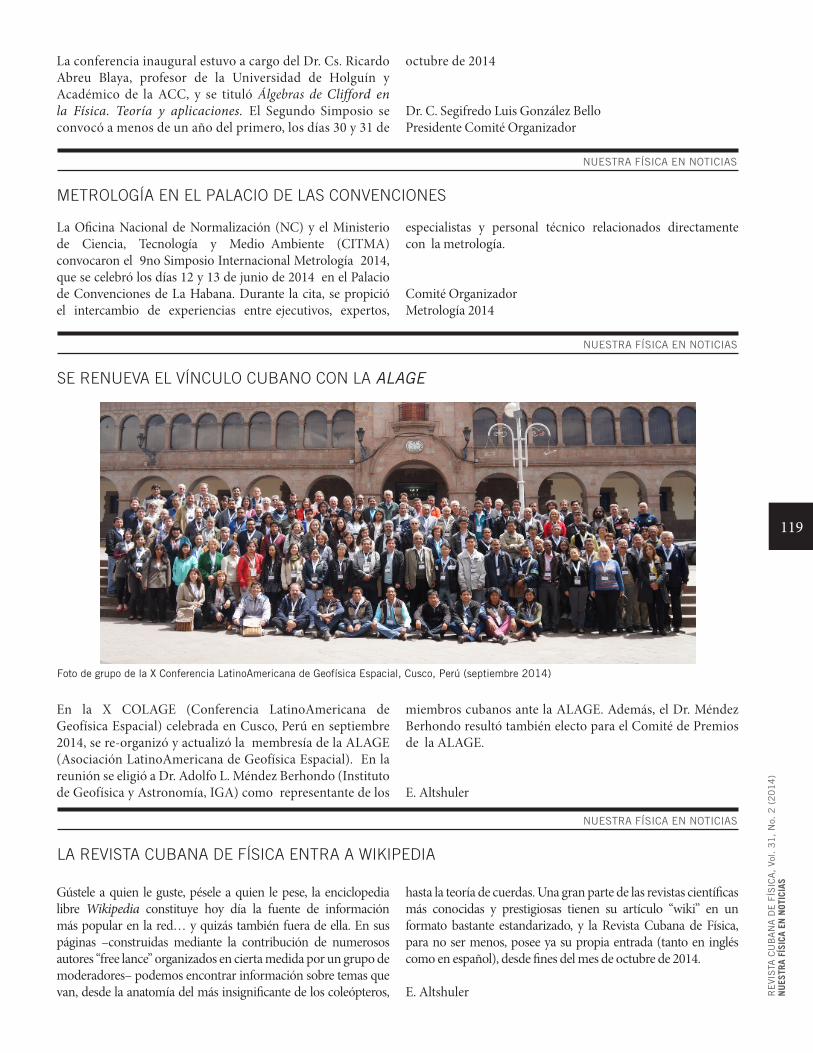
119

RE

VIS

TA C

UB

AN

A D

E F

ÍSIC

A,

Vol. 3

1,

No.

2 (

20

14

)N

UES

TRA

FÍSI

CA E

N N

OTIC

IAS

La conferencia inaugural estuvo a cargo del Dr. Cs. Ricardo Abreu Blaya, profesor de la Universidad de Holguín y Académico de la ACC, y se tituló Álgebras de Clifford en la Física. Teoría y aplicaciones. El Segundo Simposio se convocó a menos de un año del primero, los días 30 y 31 de

octubre de 2014

Dr. C. Segifredo Luis González BelloPresidente Comité Organizador

NUESTRA FÍSICA EN NOTICIAS

METROLOGÍA EN EL PALACIO DE LAS CONVENCIONES

La Oficina Nacional de Normalización (NC) y el Ministerio de Ciencia, Tecnología y Medio Ambiente (CITMA) convocaron el 9no Simposio Internacional Metrología 2014, que se celebró los días 12 y 13 de junio de 2014 en el Palacio de Convenciones de La Habana. Durante la cita, se propició el intercambio de experiencias entre ejecutivos, expertos,

especialistas y personal técnico relacionados directamente con la metrología.

Comité OrganizadorMetrología 2014

NUESTRA FÍSICA EN NOTICIAS

SE RENUEVA EL VÍNCULO CUBANO CON LA ALAGE

En la X COLAGE (Conferencia LatinoAmericana de Geofísica Espacial) celebrada en Cusco, Perú en septiembre 2014, se re-organizó y actualizó la membresía de la ALAGE (Asociación LatinoAmericana de Geofísica Espacial). En la reunión se eligió a Dr. Adolfo L. Méndez Berhondo (Instituto de Geofísica y Astronomía, IGA) como representante de los

Foto de grupo de la X Conferencia LatinoAmericana de Geofísica Espacial, Cusco, Perú (septiembre 2014)

miembros cubanos ante la ALAGE. Además, el Dr. Méndez Berhondo resultó también electo para el Comité de Premios de la ALAGE.

E. Altshuler

NUESTRA FÍSICA EN NOTICIAS

LA REVISTA CUBANA DE FÍSICA ENTRA A WIKIPEDIA

Gústele a quien le guste, pésele a quien le pese, la enciclopedia libre Wikipedia constituye hoy día la fuente de información más popular en la red… y quizás también fuera de ella. En sus páginas –construidas mediante la contribución de numerosos autores “free lance” organizados en cierta medida por un grupo de moderadores– podemos encontrar información sobre temas que van, desde la anatomía del más insignificante de los coleópteros,

hasta la teoría de cuerdas. Una gran parte de las revistas científicas más conocidas y prestigiosas tienen su artículo “wiki” en un formato bastante estandarizado, y la Revista Cubana de Física, para no ser menos, posee ya su propia entrada (tanto en inglés como en español), desde fines del mes de octubre de 2014.

E. Altshuler

120

RE

VIS

TA C

UB

AN

A D

E F

ÍSIC

A,

Vol. 3

1,

No.

2 (

20

14

)N

UES

TRA

FÍSI

CA E

N N

OTIC

IAS

La Revista Cubana de Física en Wikipedia. Además de una sucinta información sobre los objetivos básicos de la revista y las bases de datos donde se encuentra indizada, el artículo contiene, en su margen derecho, una gran cantidad de información bibliográfica clave sobre la revista, de forma concisa.

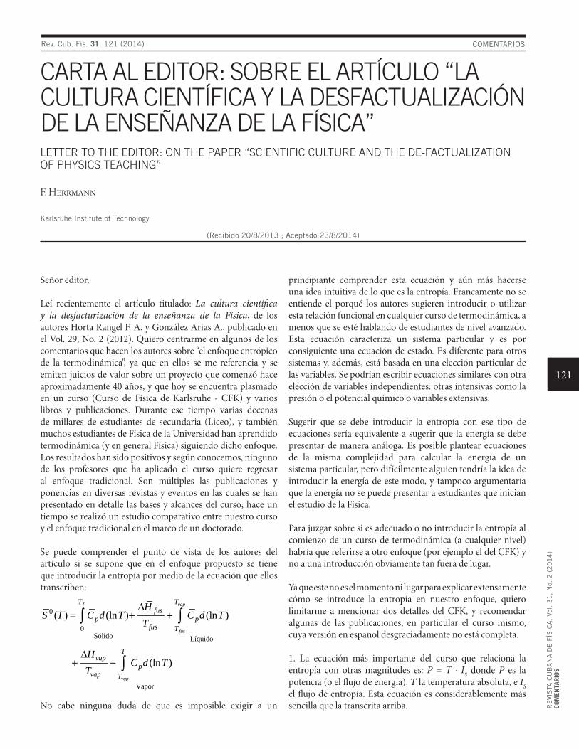
121

RE

VIS

TA C

UB

AN

A D

E F

ÍSIC

A,

Vol. 3

1,

No.

2 (

20

14

)CO

MEN

TARI

OS

COMENTARIOS

CARTA AL EDITOR: SOBRE EL ARTÍCULO “LA CULTURA CIENTÍFICA Y LA DESFACTUALIZACIÓN DE LA ENSEÑANZA DE LA FÍSICA”LETTER TO THE EDITOR: ON THE PAPER “SCIENTIFIC CULTURE AND THE DE-FACTUALIZATION OF PHYSICS TEACHING”

F. Herrmann

Karlsruhe Institute of Technology

(Recibido 20/8/2013 ; Aceptado 23/8/2014)

Señor editor,

Leí recientemente el artículo titulado: La cultura científica y la desfacturización de la enseñanza de la Física, de los autores Horta Rangel F. A. y González Arias A., publicado en el Vol. 29, No. 2 (2012). Quiero centrarme en algunos de los comentarios que hacen los autores sobre “el enfoque entrópico de la termodinámica”, ya que en ellos se me referencia y se emiten juicios de valor sobre un proyecto que comenzó hace aproximadamente 40 años, y que hoy se encuentra plasmado en un curso (Curso de Física de Karlsruhe - CFK) y varios libros y publicaciones. Durante ese tiempo varias decenas de millares de estudiantes de secundaria (Liceo), y también muchos estudiantes de Física de la Universidad han aprendido termodinámica (y en general Física) siguiendo dicho enfoque. Los resultados han sido positivos y según conocemos, ninguno de los profesores que ha aplicado el curso quiere regresar al enfoque tradicional. Son múltiples las publicaciones y ponencias en diversas revistas y eventos en las cuales se han presentado en detalle las bases y alcances del curso; hace un tiempo se realizó un estudio comparativo entre nuestro curso y el enfoque tradicional en el marco de un doctorado.

Se puede comprender el punto de vista de los autores del artículo si se supone que en el enfoque propuesto se tiene que introducir la entropía por medio de la ecuación que ellos transcriben:

0

0Sólido Líquido

Vapor

( ) (ln ) (ln )

(ln )

f vap

fus

vap

T Tfus

p pfus T

Tvap

pvap T

HS T C d T C d T

T

HC d T

T

∆= + +

∆+ +

∫ ∫

∫

No cabe ninguna duda de que es imposible exigir a un

principiante comprender esta ecuación y aún más hacerse una idea intuitiva de lo que es la entropía. Francamente no se entiende el porqué los autores sugieren introducir o utilizar esta relación funcional en cualquier curso de termodinámica, a menos que se esté hablando de estudiantes de nivel avanzado. Esta ecuación caracteriza un sistema particular y es por consiguiente una ecuación de estado. Es diferente para otros sistemas y, además, está basada en una elección particular de las variables. Se podrían escribir ecuaciones similares con otra elección de variables independientes: otras intensivas como la presión o el potencial químico o variables extensivas.

Sugerir que se debe introducir la entropía con ese tipo de ecuaciones sería equivalente a sugerir que la energía se debe presentar de manera análoga. Es posible plantear ecuaciones de la misma complejidad para calcular la energía de un sistema particular, pero difícilmente alguien tendría la idea de introducir la energía de este modo, y tampoco argumentaría que la energía no se puede presentar a estudiantes que inician el estudio de la Física.

Para juzgar sobre si es adecuado o no introducir la entropía al comienzo de un curso de termodinámica (a cualquier nivel) habría que referirse a otro enfoque (por ejemplo el del CFK) y no a una introducción obviamente tan fuera de lugar.

Ya que este no es el momento ni lugar para explicar extensamente cómo se introduce la entropía en nuestro enfoque, quiero limitarme a mencionar dos detalles del CFK, y recomendar algunas de las publicaciones, en particular el curso mismo, cuya versión en español desgraciadamente no está completa.

1. La ecuación más importante del curso que relaciona la entropía con otras magnitudes es: P = T · IS donde P es la potencia (o el flujo de energía), T la temperatura absoluta, e IS el flujo de entropía. Esta ecuación es considerablemente más sencilla que la transcrita arriba.

Rev. Cub. Fis. 31, 121 (2014)

122

RE

VIS

TA C

UB

AN

A D

E F

ÍSIC

A,

Vol. 3

1,

No.

2 (

20

14

)CO

MEN

TARI

OS

2. Se presenta un método de medición de la entropía que no requiere utensilios diferentes a los que se pueden encontrar en cualquier hogar.

Puede encontrarse amplia bibliografía en varios idiomas en el siguiente sitio:http://www.physikdidaktik.uni-karlsruhe.de/

Material en español:http://www.physikdidaktik.uni-karlsruhe.de/publication/pub_fremdsprachen/spanisch.html

Bases generales de la parte termodinámica del curso:http://www.physikdidaktik.uni-karlsruhe.de/publication/job-

termodinamica.pdf

Versión incompleta del curso en español: http://www.physikdidaktik.uni-karlsruhe.de/kpk/spanisch/kpk_estud.pdf

Sobre la medición de la entropía:http://formacionvirtual.redp.edu.co/mod/resource/view.php?id=184http://www.physikdidaktik.uni-karlsruhe.de/publication/Historical_burdens/30_Measuring_entropy.pdf

Trabajo de evaluación del curso (tesis de doctorado):http://www.logos-verlag.de/cgi-bin/buch/isbn/823

123

RE

VIS

TA C

UB

AN

A D

E F

ÍSIC

A,

Vol. 3

1,

No.

2 (

20

14

)CO

MEN

TARI

OS

COMENTARIOS

CARTA AL EDITOR: RESPUESTA AL COMENTARIO DE F. HERRMANNLETTER TO THE EDITOR: REPONSE TO F. HERRMANN’S COMMENT

A. González Arias y F. A. Horta Rangel

(Recibido 22/10/2014 ; Aceptado 25/10/2014)

Estimado editor de la Revista Cubana de Física:

Somos de la opinión de que ya es hora de que la Pedagogía asuma el papel de Ciencia que usualmente se le atribuye. La ciencia no es cuestión de criterios y opiniones, sino de demostraciones basadas en la evidencia. Si es mediante el experimento controlado, mejor.

El Dr. Herrmann menciona un proyecto que afirma lleva 40 años de existencia, plasmado en un curso, libros y publicaciones (posiblemente de su creación o como profesor principal) con resultados positivos. Desafortunadamente, no cita o menciona estadísticas que muestren que este enfoque resulta mejor para el estudiante que el tradicional (o, por ejemplo, resultados de evaluaciones realizadas por profesores independientes).

En su comentario el Dr. Herrmann tampoco toma en cuenta que el aprendizaje depende de forma muy importante de la historia o preparación previa del estudiante. Está fuera de discusión que no se obtendrán los mismos resultados cuando aplique su método a estudiantes alemanes o a estudiantes de Haití o de Sierra Leona. Aparentemente, en su opinión, su método es igualmente eficiente para todos.

Otro aspecto a mencionar es que en repetidas ocasiones hemos visto que el afán por simplificar la física en la enseñanza media conduce a serios errores conceptuales. Se le imparten al estudiante conceptos más simples de comprender, pero erróneos, que obviamente serán muy difíciles de corregir en el futuro.

El Dr. Herrmann malinterpreta nuestros comentarios sobre la entropía cuando afirma que nosotros proponemos que se introduzca el concepto mediante una ecuación compleja, para después criticar lo que no hemos dicho. Lo que se dice allí es precisamente lo contrario: que la entropía es una magnitud compleja (y para eso se muestra como ejemplo la ecuación citada) y que no parece adecuado comenzar el estudio de la Termodinámica a partir de la entropía, justamente por la complejidad del concepto.

No deseamos repetir los argumentos que aparecen en la página 65 de nuestro artículo, que reafirmamos. Guste o no, la entropía es una función de estado del sistema. Eso hay que decirlo de alguna manera para no incurrir en la impartición de conceptos incorrectos al estudiante. Y, desde luego, no es la única función de estado. Si no se muestra de antemano por qué es una función de estado, no quedará más remedio que dibujar alguna ecuación y decirle al estudiante que eso es una función de estado, cayendo de lleno en la desfactualización de la enseñanza de la física, tema principal del artículo.

Por otro lado, el Dr. Herrmann no comparte la visión moderna de conceptos como calor (transferencia de energía en forma microscópica y desordenada) pues critica el concepto clásico del calor, no el moderno, ya que incluso no menciona este último en su libro Conceptos obsoletos en Física, Colección Tierra y Vida, Ed. UD, Colombia, 2011 (p.93) o el de "función de estado del sistema", que denomina "magnitud de estado" (p.77). Solamente recomienda eliminarlas por no ser necesarias (lo cual equivale, en nuestra opinión, a negar el primer principio y la visión microscópica del universo). Al analizar la medición de la entropía, aparentemente no le preocupan aspectos tales como la entropía de mezcla o la ecuación de Planck-Boltzmann. Podríamos decir que, calentando agua con una resistencia resuelve el problema del cálculo de la entropía (p. 83).

La entropía tampoco es un fluido que se transmite de un sistema a otro -criterio que lamentablemente aún se maneja en algunos lugares, en forma figurada al parecer- sino algo más complejo, imposible de comprender mediante un ejemplo muy particular, que creemos tiende a oscurecer la riqueza y complejidad del concepto. En la ciencia la inmensa mayoría de las veces (y especialmente en la Termodinámica) el experimento viene primero; la teoría, después. Según el Dr. Herrmann, la ecuación más importante del curso es la que relaciona la entropía con otras magnitudes es P = T · IS. Los abajo firmantes seguimos creyendo que la ley cero, la 1ra, 2da y 3ra leyes conducen a las ecuaciones más importantes en un curso de Termodinámica, junto a la imposibilidad de crear móviles perpetuos: estas ecuaciones no han pasado de moda,

Rev. Cub. Fis. 31, 123 (2014)

124

RE

VIS

TA C

UB

AN

A D

E F

ÍSIC

A,

Vol. 3

1,

No.

2 (

20

14

)CO

MEN

TARI

OS

y es crucial transmitirlas a las nuevas generaciones. Por otra parte ¿las leyes no surgieron por un proceso de inducción?

La entropía tiene tres acepciones diferentes, cada una con sus especificidades y descripción matemática cuya relación no es evidente, ni mucho menos:

1. Es una medida de la pérdida de capacidad de un sistema para convertir su energía en trabajo útil (degradación de la energía).

2. Es una medida del ‘grado de orden’ de un sistema.3. Es una medida de la espontaneidad de un proceso y del

estado de equilibrio de un sistema.

Reducir todo esto a un criterio de flujo, tratando de imitar los conceptos alegóricos de la termodinámica de los procesos irreversibles, nos parece poco feliz como elemento educativo. En todo caso, quien propone el enfoque novedoso es quien debería demostrar su validez.

Reconocemos que es probable que los alumnos memoricen mejor los ‘nuevos’ conceptos propuestos y que algunos profesores se sientan muy a gusto con los resultados, pero pensamos que también es seguro que al final del curso los estudiantes sabrán mucho menos física que los que reciben los cursos tradicionales. A nuestro modo de ver, no hace falta realizar experimentos controlados para llegar a esta conclusión.

Revista Cubana de FísicaImpresa: ISSN 0253 9268En línea: ISSN 2224 9268