3. JIT• 27·7·10

Joumal of Industrial Technology (25-32)

THE FLYING VEHICLE FLIGHT TRAJECTORY OPTIMIZATION (THREE-DIMENSIONAL MOTION)

V. P. Nesterov

School of Aerospace Engineering, Engineering Campus, Universiti Sains Malaysia, Seri Ampangan,

14300 Nibong Tebal, Pulau Pinang, Malaysia (vpnesterov@mail.ru)

RINGKASAN : Satu teknik rekabentuk dicadangkan untuk perpindahan optima dari

keadaan mu/a dan akhir di dalam ruang tiga dimensi, di tengah medan graviti, di dalam

ruang kosong, dan di bawah pergerakan tujahan yang tetap. Kajian ini merangkumi

algorisma kawalan pergerakan kenderaan yang dibina me/alui Teori Gunaan Kawa/an

Optima. Perubahan sudut serangan a(t) dan sudut golekan halaju Yv(t) dibandingkan

dengan masa penerbangan kenderaan ditunjukkan pada nilai kecondongan yang diberi.

Variasi nilai penambahan kos untuk karakterha/aju pada akhirpenerbangan dan lebihan

perubahan antara jisim akhir kenderaan terbang untuk kecondongan lli .. o dan untuk

lli = o bergantung kepada nilai kecondongan L1i di bawah kawalan optima (sudut

serangan dan sudut ha/aju go/ekan) juga <illunjukkan.

ABSTRACT : A design technique is suggested for the flying vehicle optimal transfer

from the initial to a final state in three-dimensional space, in the central gravitation field,

in empty space and under the action of fixed thrust. The given study considers the

flying vehicle motion control algorithm built proceeding from the optimal control applied

theory. The changes of the angle of attack a(t) and velocity roll angle yv(t) versus the

flying vehicle flight time are presented for the given inclination value. A value variation

of additional costs of the characteristic velocity at the end of flight and a residue change

between the flying vehicle final mass for inclination lli .. o and for lli = o depending on

inclination value ru under optimal control (the angle of attack and velocity roll angle)

are also shown.

KEYWORDS : Three-dimensional motion, optimal control, flying vehicle, equations of

flying vehicle motion, angle of attack, velocity roll angle

25

V. P. Nesterov

INTRODUCTION

Nesterov (2009) suggested a design procedure for the flying vehicle (FV) optimal transfer

from the initial to a final state in one plane, in the central gravitation field, in empty space and

under the action of fixed thrust. FV control is performed by the angle of attack. In a given

study, a design procedure for the FV optimal transfer from the initial to a final state in three­

dimensional space is proposed. FV control is performed by the angle of attack and velocity

roll angle.

METHODOLOGY

The present study considers the design technique of the flying vehicle (FV) optimal transfer

under the action of constant thrust exceeding the Newtonian force, from initial to final state,

characterized by prescribed values of FV radius-vector relative to the attracting centre, velocity,

angle of inclination of the velocity vector to a local horizon and trajectory inclination.

The following assumptions were made:

(i) the Earth is of a spherical shape and during the transfer phase it does not rotate,

(ii) its gravity field is central,

(iii) the FV flight runs at high altitudes where air resistance is negligible and

(iv) the FV control system is inertialess.

The algorithm analysis of FV optimal transfer trajectory is built based on the applied theory

of optimal control (Bryson & Ho, 1969), (Nesterov, 2009).

The equations of FV motion in its centric rectangular vertical-wind-body coordinate system

are used according to Gorbatenko et al. (1969)

. x = ](x,ii,t). (7 equations) (1)

26

The Flying Vehicle Flight Trajectory Optimization (Three-Dimensional Motion)

2

dV p (Ro) . 0· - =-COSCX-g - sm ' dt m O R

2

d0 P . (R ) 0 V - = - sm acosy · g - 0 cos + - cos 0; dt mV v O R V R

~ = _ .!.._ sin a sin 'Yv dt mV cos 0

dR V . 0 dt= sm ;

dm V ..::..z. = -R cos 0 cos '" · dt T v•

+ ~ cos 0 X tg<p X sin 'l'v ; R

d).,,' v . dt = -R cos0 sm 'lfvsec <p;

dm a. -=-m' dt

(2)

where x = (V ,0, 'l'v, R,q,,'Ji: ,m)T is the FV current state vector,f(x,u-,t) is the vector of the right

sides of the system of differential equations of vehicle's motion, t is the current time of the

flight, Vis the vehicle's velocity, 0 is the velocity vector angle of inclination to a local horizon,

'l'v is the velocity heading angle, R is the value of FV radius-vector relative to the attracting

centre, q> is the geocentric latitude, 'Ji: is the geocentric longitude, m is the FV mass, P is the R 2

FV thrust value, g0 is the free-fall acceleration value on Earth's surface, g = g0 ( R0) is the

. free-fall acceleration value at vehicle's attitude, R0 is the Earth's radius, m• is the absolute

value of FV mass flow, a is the angle of attack and Yv is the velocity roll angle.

For parameters of FV motion control we use the angle of attack and the velocity roll angle:

u(t) = ( a(t), Yv<tW. (3)

The FV initial state vector is prescribed:

x (t.). (7 initial conditions). (4)

27

V. P. Nesterov

The FV terminal state is confined as

(5)

where t r is the current time at the end of flight,

where '1'1 = V- Ve - by the velocity vector value at the end of transfer leg, '1'2 = 0- er - by the value

of inclination angle of velocity vector to a local horizon at the end of the transfer leg, '1'3 = R - Rr -

by FV radius-vector value relative to the attracting centre at the end of the transfer leg,'1'4= i- i r­

by the inclination value i .

The negative final mass is the FV performance criterion:

- m(tr) . (6)

So, the task is to define such a control u (t) , which could provide the minimum of negative

value of final mass [- m(tr )] with available differential constraints (1) and limitations to a

terminal state (5). The Hamiltonian H (Bryson & Ho, 1969) for this task can be written as:

(7)

-where 11. = (11.1 , \ , \ , 11.4 , \, \ , \ Y - the Lagrangian multiplier vector (function interference

vector upon the functional).

The Euler- Lagrange set of equations looks like:

cJH =0, ou

Terminal conditions give us the equalities:

28

(7 equations), (8)

(2 equations), (9)

(7 conditions), (10)

The Flying Vehicle Right Trajectory Optimization (Three-Dimensional Motion)

(11)

,.; - - (dct>j OtX,U, v,t],=tf = - = 0, dt 1=1r (1 condition) (12)

Time of transfer ending tr is determined implicitly by means of terminal boundary conditions

(10).

From equations (7) and (8), we can write down:

oT __ -:;T]J_ x - 11,(fx · (13)

Thus, it is required to find a solution of the system of 14 differential equations (1) (set of

equations of flying vehicle motion) and (8) (set of equations of costate variables) and determine 5 values of unknown parameters v and tr so that to meet seven initial conditions (4) and twelve terminal conditions (5), (10), (12). Determination of u (t) is made using the equations

(9):

yVI = arctg[- x;~~se], (-1t:::;; Yv::s; 7t ),

(14)

Yvi = YVI + 7t.

For each value Yv we determine two values of the angle of attack:

l sin Yv a 1 = arctg[~ V (A:iCOS Yv-11,3--8 )],

11,1 cos (15)

A According to Bryson & Ho (1969), the time optimal control u should minimize H (u):

A A- -

H(i,u,A,t)::s; H (x,u,A,t) .

Solution of the equations (1) - (12) can be reduced to a solution of nine-parametric boundary­value equations (Smirnov & Nesterov, 1980) which is reduced to a finding of roots of a set of

equations:

V0 = V(ic),00 = 0(ic);1Jfvo= 'lf/K"),R0= R(ic),<f>o = <p(K), A.10= A'(ic), m0= m(ic), i'= i(ic),08 = Q(ic),

29

(16)

V. P. Nesterov

where ic = ( tf' v., v2 , 'l'vf, v3 , <pf' 'A.'f' mf' v4 ) is a vector of unknown parameters. (17)

Here: V0 ,00 ,'l'vo ,R0 ,'A,'0 , m0 are given values of FV parameters to the time, t0 • They must be

found when solving a boundary-value problem; i',Q are given values of inclination and g

parameter Q (from condition (12)).

Integration of the system of differential equations (1) and (13) are performed with a negative

step until the time t 0 , then we find the discrepancies by conditions (16). Solution of the boundary­

value problem runs until the conditions (16) be met with a given accuracy. To solve the boundary­

value problem we make use of the Newton method for solution of the system of nonlinear

equations. In the case that we know well enough the initial approximations of Lagrangian

multiplier vector "X(t0 ), the solution of the problem (1)-(12) can be reduced to a finding of five

roots of a set of equations:

0r= 0(cr), Rr = R(cr),i' = i(cr),O = i\v/cr),Q.8 = Q(cr), (18)

(19)

Here, er , Rf' i' are given values of FV parameters to the time moment tr and inclinations to

be performed in consequence of boundary-value problem solving, Q& is obtained from (12),

i\v4 is obtained from (10).

When taking into account that in (10) \(tr)= v4 i'., ,\(t;) = v4 ~i , V'j' V <p

'A.itr) 'A.s(tr) we get i\v = .

4 (difd'lfv) (di/d<p)

In this case, integration of the system of differential equations (1) and (13) are performed

with a positive step from the time, t O until the fulfilment of prescribed condition by velocity at

the end of transfer V = V r• and then we determine the residuals by conditions in (18). V = V r

is the sixth condition in addition to condition (18), hence we solve a six-parametric boundary­

value problem.

RESULTS

The given study considers the FV motion control algorithms built proceeding from the optimal­

control applied theory. FV control is performed by angle of attack and velocity roll angle.

30

ao 60

0 100

The Aying Vehicle Right Trajectory Optimization (Three-Dimensional Motion)

Y: - 30

200 300 t,s

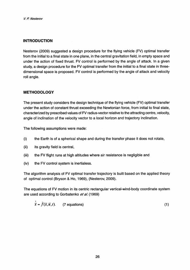
Figure 1. The angle of auack and velocity roll angle variation

Figure 1 illustrates the changes of the angle of attack a(t) and velocity roll angle yy(t) depending on the FV flight time for Iii = 25° .

!Nx1, m/s ~mr, kg

100 2000

so 1000

~i, deg -12 -10 -8 -6 -4 -2 0 2 4 6 8 10 12

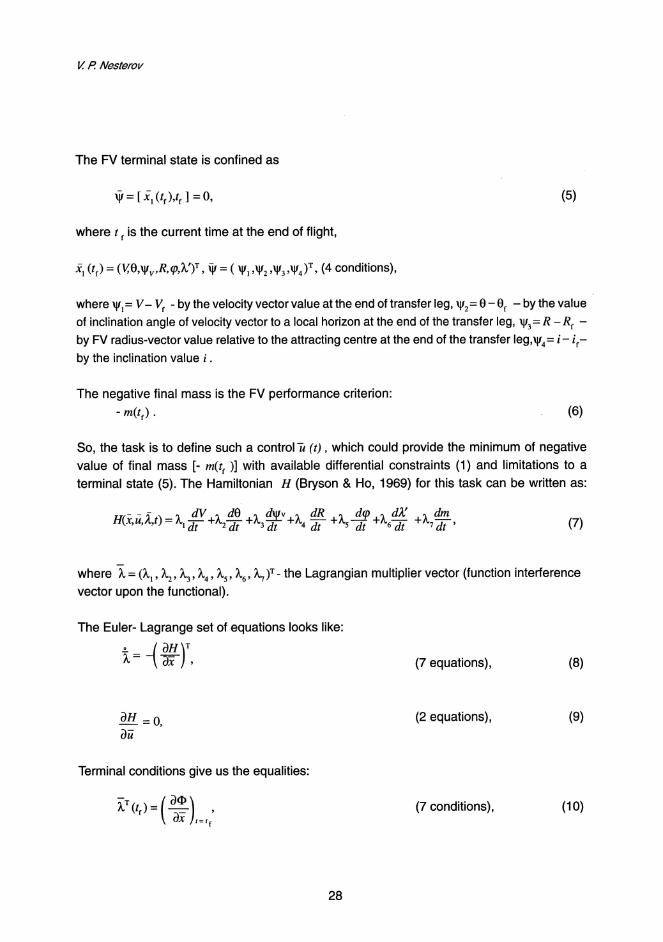
Figure 2. Value of variation of additional costs of the characteristic velocity at the end of flight showing the dependence on the inclination value f!...i under optimal control

31

V. P. Nesterov

Figure 2 illustrates a value variation of additional costs of the characteristic velocity at

the end of flight (AVx1 = Vx1 (Ai)-Vx1 (Ai= 0)) and a residue change

(L\mr = mr (L\i) - m/L\i = 0 )) between the FV final mass for inclination Ai _. 0 and for

Ai = 0 depending on the inclination value Ai under optimal control (the angle of attack

and velocity roll angle).

CONCLUSION

Thus, in this investigation a design procedure was suggested and realized in the software

modules using the Fortran-IV algorithmic language for the flying vehicle optimal transfer

from the initial to a final state in three-dimensional space, in the central gravitation field, in

empty space and under the action of fixed thrust. This investigation reveals the changes of

the angle of attack a(t) and velocity roll angle yy(t) versus the flying vehicle flight time which

are presented for the given inclination value. A value variation of additional costs of the

characteristic velocity at the end of flight and a residue change between the flying vehicle

final mass for inclination Ai ,. O and for Ai = O depending on inclination value Ai under

optimal control are also shown.

REFERENCES

Bryson, A. E., Ho You-Chi. (1969). Applied optimal control. Blaisdell Publishing Company,

London. pp 42-89.

Gorbatenko S.A., Makashov E.M., Polushkin Yu. F., Sheftel L. V. (1969). Flight mechanics.

Engineering Handbook. Mashinostroenie, Moscow. pp 129, 188-189.

Nesterov V. P. (2009). The Flying Vehicle Optimum Flight Trajectory Design. Journal of

Industrial Technology. Vol. 18(1):pp 33-40.

Smirnov 0. L., Nesterov V. P. (1980). The Investigation of Guidance Algorithms During Landing

A Vehicle with the Radio Beacon. XXXI Congress of the International Astronautical Federation.

Abstracts of Papers. Tokyo, Japan. pp 248.

32