UNIVERSITI PUTRA MALAYSIA

EM APPROACH ON INFLUENCE MEASURES IN COMPETING RISKS VIA PROPORTIONAL HAZARD REGRESSION MODEL

FAIZ. A. M. ELFAKI

FSAS 2000 5

EM APPROACH ON INFLUENCE MEASURES IN COMPETING RISKS VIA

PROPORTIONAL HAZARD REGRESSION MODEL

F AIZ. A. M. ELF AKI

MASTER OF SCIENCE

UNIVERSITI PUTRA MALAYSIA

2000

EM APPROACH ON INFLUENCE MEASURES IN COMPETING RISKS VIA PROPORTIONAL HAZARD REGRESSION MODEL

By

FAIZ. A. M. ELFAKI

Thesis Submitted in Fulfilment of the Requirements for the Degree of Master of Science in the Faculty of

Science and Environmental Studies Universiti Putra Malaysia

June 2000

Dedicated to my late mother, Etayah Mohamed Abdullah, May Allah rest her soul in heaven

II

Abstract ofthesis submitted to the Senate ofUniversiti Putra Malaysia in fulfilment of the requirements for the degree of Master of Science

EM APPROACH ON INFLUENCE MEASURES IN COMPETING RISKS VIA PROPORTIONAL HAZARD MODEL

By

FAIZ AHMED MOHAMED ELFAKI

Jun e 2000

Chairman: Noor Akma Ibrahim, Ph.D.

Faculty: Sci enc e and Environm ental Studi es

In a conventional competing risks model, the time to failure of a particular

experimental unit might be censored and the cause of failure can be known or

unknown. In this thesis the analysis of this particular model was based on the

cause-specific hazard of Cox model. The Expectation Maximization (EM) was

considered to obtain the estimate of the parameters. These estimates were then

compared to the Newton-Raphson iteration method. A generated data where the

failure times were taken as exponentially distributed was used to further compare

these two methods of estimation. From the simulation study for this particular case,

we can conclude that the EM algorithm proved to be more superior in terms of

mean value of parameter estimates, bias and root mean square error.

111

To detect irregularities and peculiarities in the data set, the residuals, Cook

distance and the likelihood distance were computed. Unlike the residuals, the

perturbation method of Cook's distance and the likelihood distance were effective

in the detection of observations that have influenced on the parameter estimates.

We considered both the EM approach and the ordinary maximum likelihood

estimation (MLE) approach in the computation of the influence measurements. For

the ultimate results of influence measurements we utilized the approach of the one­

step . The EM one-step and the maximum likelihood (ML) one-step gave

conclusions that are analogous to the full iteration distance measurements. In

comparison, it was found that EM one-step gave better results than the ML one­

step with respect to the value of Cook's distance and likelihood distance. It was also

found that Cook's distance is better than the likelihood distance with respect to the

number of observations detected.

iv

Abstrak tesis yang dikemukakan kepada Senat Universiti Putra Malaysia sebagai memenuhi keperluan untuk Ijazah Master Sains

P END EKATANP EMAKS�UMANJANGKAANT ERHADAP UKURAN

P ENGARUH DALAM RISIKO B ERSAING MENERUSI MOD EL KADARANBAHAYA

Ol eh

FAIZ AHMED MOHAMED ELFAKI

Jun 2000

Peng erusi: Noor Akma Ibrahim, Ph.D.

Fakulti: Sains dan Pengajian Alam S ekitar

Dalam model risiko bersaing konvensional, masa kegagalan dari unit ujikaji

tertentu boleh jadi tertapis dengan punca kegagalan mungkin diketahui atau tidak

diketahui. Dalam tesis ini analisis model risiko bersaing adalah berlandaskan model

bahaya punca-tertentu Cox. Pemaksimuman Jangkaan (PJ) dipertimbangkan untuk

memperolehi anggaran bagi parameter. Anggaran ini dibandingkan dengan

anggaran yang diperolehi dari kaedah lelaran Newton-Raphson. Data yang dijana

dengan masa kegagalannya tertabur secara eksponen digunakan selanjutnya untuk

membandingkan kedua-dua kaedah anggaran ini. Dari kajian simulasi khususnya

bagi masalah ini, didapati algoritma PI mempunyai kelebihan terhadap anggaran

v

parameter berdasarkan nilai mm, kepincangan dan punca kuasa dua min ralat

(PKMR).

Untuk melihat ketidaktentuan dan keganjilan data dalam model, reja, jarak

Cook dan jarak kebolehjadian dihitung. Tidak seperti reja, kaedah jarak Cook dan

jarak kebolehjadian adalah berkesan dalam menentukan cerapan yang

mempengaruhi anggaran parameter. Kedua-dua pendekatan iaitu PJ dan anggaran

maksimum kebolehjadian dilaksanakan dalam perhitungan ukuran pengaruh.

Sebagai keputusan muktamad ukuran pengaruh, satu-Iangkah digunakan. PJ satu­

langkah dan kebolehjadian maksimum (KM) satu-langkah memberikan kesimpulan

yang sama dengan ukuran jarak lelaran penuh. Secara perbandingan, didadapati

bahawa PJ satu-Iangkah memberikan keputusan yang lebih baik daripada KM satu­

langkah berdasarkan nilai jarak Cook dan jarak kebolehjadian yang diperolehi. Juga

didapati bahawa jarak Cook adalah lebih baik daripada jarak kebolehjadian dari

segi bilangan cerapan yang dikesan sebagai berpengaruh.

vi

ACKNOWLEDGEMENTS

Praise be to ALLAH for giving me the strength and patience to complete this

work. I would like to single out the particular and tremendous contribution of Dr. Noor

Akma Ibrahim, the chairman of supervisory committee, for her persistent inspiration,

constant guidance, wise counsel, encouragement, kindness, financial help and various

logistic supports during all the stages of my study. I highly appreciate her effort to give

first hand knowledge about a very interesting area of statistic. Her command on the

subject matter, together with her research experiences, have been highly valuable to my

study. In spite of her busy schedule, she managed to find enough time for my discussions

and provided necessary direction in order to develop my study. Her enthusiasm and

patience have left a feeling of indebtedness which can not be fully expressed.

My deepest appreciation and sincere gratitude also to Assoc. Prof Dr. Isa Daud,

Head of the Mathematics Department and member of my supervisory committee, for his

kind co-operation and thoughtful suggestions. lowe a great deal of gratitude and

appreciation to Mrs Fauziah Maarof, member of the supervisory committee, for her

supervision and helpful comments.

I also would like to expand my thanks to Assoc. Prof Dr. Harun bin Budin for his

help and continuous encouragement. And all the members of the Mathematics

Department for their kind assistance during my studies, particularly Dr. Jamal I. Daoud.,

Dr. Habshah Midi., Dr. Farris Assim, Mrs Fadzilah Ali and Miss Zainuridah Yusof For

vii

my friends ling Lukman, Idi Fulayi, Ahlam Abdel Hadi, Lawan Ahmed, Hanan Hassan

whatever I stated in the acknowledgement will remain under the true credit of their

genuine contribution to the success of this study. I am also thankful to Salah Madni and

his wife Ghada, Hassan Doka, Yassin Mohd, Natrah Mohd, Vema Taylor and Ahmed

Elyas, for their strong support and fast response whenever I needed their help.

Last but not the least, my heartfelt thanks should go to my father, Ahmed, my

mother, Eltayah, my brothers Abdul Gadir, Nadir, Mohamed, Mostafa and sisters, Saza,

Sara, Eltayah, Fridah, for their sacrifices, devotion and understanding, which have always

been a source of inspiration and strength throughout my life up to this moment. Also my

thanks go to all my friends in Yemen and Sudan.

Studying abroad for a prolonged period is unpleasant, if not impossible, without

friends. For all those whose names were not mentioned here, the moral support and

friendship they offered will be remembered.

viii

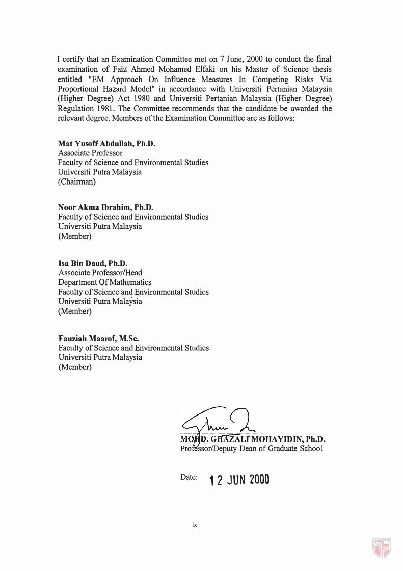
I certify that an Examination Committee met on 7 June, 2000 to conduct the final examination of Faiz Ahmed Mohamed Elfaki on his Master of Science thesis entitled "EM Approach On Influence Measures In Competing Risks Via Proportional Hazard Model" in accordance with Universiti Pertanian Malaysia (Higher Degree) Act 1980 and Universiti Pertanian Malaysia (Higher Degree) Regulation 1981. The Committee recommends that the candidate be awarded the relevant degree. Members of the Examination Committee are as follows:

Mat Yusoff Abdullah, Ph.D. Associate Professor Faculty of Science and Environmental Studies Universiti Putra Malaysia (Chairman)

Noor Akma Ibrahim, Ph.D. Faculty of Science and Environmental Studies Universiti Putra Malaysia (Member)

Isa Bin Daud, Ph.D. Associate ProfessorlHead Department Of Mathematics Faculty of Science and Environmental Studies Universiti Putra Malaysia (Member)

Fauziah Maarof, M.Sc. Faculty of Science and Environmental Studies Universiti Putra Malaysia (Member)

ZALf MOHAYIDIN, Ph.D. Pro ssorlDeputy Dean of Graduate School

Date:

ix

1 2 JUN 2000

This thesis was submitted to the Senate of Universiti Putra Malaysia and was accepted as fulfilment of the requirements for the degree of Master of Science.

x

KAM� ANG, Ph.D. Associate Professor, Dean of Graduate School, Universiti Putra Malaysia

Date: 1 3 JUL 2000

DECLARATION

I hereby declare that the thesis is based on my original work except for quotations and citations which have been duly acknowledged. I also declare that it has not been previously or concurrently submitted for any other degree at UPM or other institutions

(F AIZ AHMED MOHAMED ELFAKI)

Date: \ 1 - 6- 7.000

Xl

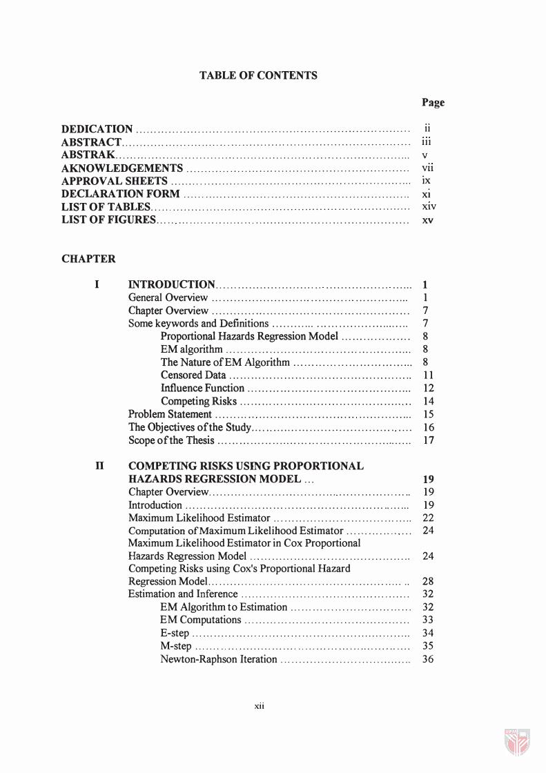
TABLE OF CONTENTS

Page

DEDICATION ..... , ., ... , ..... , ........ , ........... , ..... , .................... , ....... ,. 11

ABSTRACT ........... , ., .................. , ., ......... , .......................... , ... .... 111 ABSTRAK . . . . . . . . . . . . . . . . . . . . . . . . . . . . . . . . . . . . . . . . . . . . . . . . . . . . . . . . . . . . . . . . . . . . . . . . . . . . . . . . . v AKNOWLEDGEMENTS ........... .. . ..... . .. . .................................... .. V11 APPROVAL SHEETS ........................ '" .... , ... , ., ......... , ......... ...... ... IX DECLARA TION FORM ..... , ..... , ., .................... , ... , ........... , ........... Xl LIST OF TABLES ... '" ..................................... ,. ... ... ... ................. XIV LIST OF FIGURES ... '" .. , ............... '" .............. , ... ... ... .................. xv

CHAPTER

I INTRODUCTION . .... , .................... , '" .............. , '" ...... 1 General Overview . . , . . . . . . . . . . . . . . . . . . . . , '" . . . . . . . . . '" . . , . . . . . . . . . . . . 1 Chapter Overview ............ . . .... . , . . . . . . . . . . . . . . . . . . . . . . . . . . . . . . . . . . 7 S ome keywo rd s and Definitions . . . . . . . . . . . , . . . . . . . . . . . . . . . . . . . . . . . . . . 7

Proportional Hazards Regression Model ... . . ..... . . .. . . .. . 8 EM algorithm. . . . . . . . . . . . . . . . . . . . . . . . . . . . . . . . . . . . . . . . . . . . . . . . . . . 8 The Nature of EM Algorithm . . . . . . .. .. ... . . ... . . . . . . . . . . . . . . . 8 Censored Data . . , . . . . . . . . . . . . . . . . . . . . . . . . . . . . . . . . . . . . . . . . . . . . . . . 11 Influence Function .. . . .. . . . . . . . . . . . . . . . . . . . . . . . . . . . . . . . . . . . . ... 12 Competing Risks .. . . . . . . .. . .. . . . . . . . . . . . . . . . . . . . . .. . . . , ... '" . . 14

Problem Statement . . . . . .. .. '" . . . . . . . . . . . . . . . . . . . . . . . . '" . . . . . . . . . . . . . . . 15 The Objectives of the Study . . . '" . . . . . . . . . . . . . . . . . , . . . . . . . . . . . . . '" . . . . 16 Scope of the Thesis . .. . . . . . .. . . . .. ... .. ..... .. . . .. . . . . .. .. .. .. .. .. , . . . . . . 17

n COMPETING RISKS USING PROPORTIONAL HAZARDS REGRESSION MODEL... ... ... ... ......... ........ 19 Chapter Overview ........ .............. ........... '" . . . . . . . . . . . . . . . . . . .. 19 Introduction . . .... . . . . . . . . . . . . . . . . . . . . . . . . . . . . . . . . . . . . . . . . . . . . . . . . . . . . . . . . 19 Maximum Likelihood Estimator. . . . . . . . . . . . . . . . . . . . . . . . . . . . . . . . . . . . .. 22 Computation of Maximum Likelihood Estimator ... . , . . . . . . . '" . . . 24 Maximum Likelihood Estimator in Cox Proportional Hazards Regression Model '" ........................................ , 24 Competing Risks using Cox's Proportional Hazard Regression Model..................................................... .. 28 Estimation and Inference.............................................. 32

EM Algorithm to Estimation. . . . . . . . . . . . . . . . . . . . . . . . . . . . . . . . . 32 EM Computations . .. . . . . . . . . . . . . . . . . . . . . . . . . . . . . . . . . . . . . . . . . . . 33 E-step . .. . . . . . . . . . . . . . . . . . . . . . . . . . . . . . . . . . . . . . . . . . . . . . . . . . . . . . . . . . 34 M-step .. .... ' " . . . . . . . . . . . . . . . . . . ' " . . , . . . . . . . . . . . . . . . . . . . . . . . . . . 35 Newton-Raphson Iteration............................ . ... . . . . 36

xii

Examples and Results .. . . . . . .. . .. . . . . . . .. . ... . . ..... . . .. . . .. .. .. .. . . . .. 37 Malignant Melanoma Data . . . .............. .................. 37 Stanford Heart Transplant Data . . . . . . . . . . . . . . . . . .. . . . . . .. .... 41 Simulation Data . . . . . . . . . . . . . . . . . . . . . . . . . . . . . . . . . . . . . . . . . . . . . . . . 44

III INFLUENCE MEASURES . . . . . ... . . . . . . . . . . .. . . .. . .. . . .. . . . . . . . . . .. 51 Chapter Overview .. . .. . . . . . ... .. . .. . . . . .. . . . .. .. . . . . . . .. . . .. . . . . . . . .. . . . 5 1 Introduction . .. . . . . . . . . . . . . .. . . . . . . . . . .. .. . . . .. . ... . . . .. . . . . . . . . . . . . .. ... . 51 Influence Measurement . . .. . . . . . . . . .. . . . .. . . . . . . . . . . . . . . . . . . . . . . . . . . . . .

Cook's Distance . . . . . . . . . . . . . . . . . . . . . . . . . . . . . . . . . . . . . . . . . . . . . . . Likelihood's Distance . . . . . . . . . . . . . . . . . . . . . . . . . . . . . . . . . . . . . . . . , .

Methods for Estimation . . . . . . . . . . . . . . . . . . . . . . . . . . . . . . . . . . . . . . . . .. . . . . . . . One -step EM . . . . . . . . . . . . . . . . . . . . . . . . . . . . . . . . . . . . . . . . . . . . . . . . . . One-step ML . . . . . . . . . . . . . . . . . . . . . . . . . . . . . . . . . . . . . . . . . . . . . . . . . . .

Examples and Results . . . . . . . . . . . . . . . . . . . . . . . . . . . . . . . . . . . . . . . . . . . . . . . . . . Malignant Melanoma Data . . . . . . . . . . . . . . . . . . . . . . . . . . . . . . . . . . . Stanford Heart Transplant Data . . . . . . . . . . . . . . . . . . . . . . . . . . . . . . Simulation Data . . . . . . . . . . . . . . . . . . . . . . . . . . . . . . . . . . . . . . . . . . . . . . . .

IV CONCLUSION AND SUGGESTIONS FOR

53 54 55 56 58 59 60 60 66 71

FURTHER RESEARCH............................................. 101 Conclusion . . . . . . . . . . . . . . . . . . . . . . . . . . . . . . . . . . . . . . . . . . . . . . . . . . . . . . . . . . . . . . . 101 Suggestions for Further Research. . . . . . . . . . . ... . . . . . . . . . . . . . . . . . . . . . . . 1 04

BIBLIOGRAPHy........................................................................ 105

APPENDICES............................................................................. 1 15 Appendix I . . .... . .... . . . . . ...... . . ............ . ............. . . ........ 1 16 Appendix II .. ... . .. . . . . ... . .......... . . ............ . ........... . ...... 1 1 6

VITA . . . .... . . . . . . . . . . . . . . . . . . . . . . . . . . . . . . . . . . . . . . . . . . . . . . . . . . . . . . . . . . . . . . . . . . . . . . . . . . . . . . . . . 1 17

XIII

LIST OF TABLES

Table Page

1 A comparison of the EM algorithm and ML estimates with the estimates obtained under the Cox's model. Also shown is Andersen. et aI, consistent estimates of parameter and standard error of parameter. . . . . . . . . . . . . . . . . . . . . . . . . . . . . . . . . . . . . . . . . . . . . . . . . . . . . 40

2 A comparison of Larson and Dinse estimates with the estimates obtained under Cox's model by using the EM algorithm and ML methods. . . . . . . . . . . . . . . . . . . . . . . . . . . . . . . . . . . . . . . . . . . . . . . . . .. . . . . . . . . . 43

3 Results from simulation 1 -4 comparing the EM algorithm method, with ML method, under the Cox's model . . . . . . . . . . . . . . . .. 48

4 Cook's distance and likelihood distance from Stanford Heart Transplant data obtained by full iteration (EM and ML) under competing risk model . . . . . . . . . . . . . . . . . . . . . . . . . . . . . . . . . . . . . . . . . . . . . . . . . . . 68

5 Cook's distance and Likelihood distance obtained by one-step EM and one-step ML under competing risk model from simulation 1 (sample size 1 5) . . . . .. . . . . . . . . . . . . . . . . . . . . . . . . . . . .. .. . . . . 72

6 Cook's distance and Likelihood distance obtained by one-step EM and one-step ML under competing risk model from simulation 2 (first risk)........ . .. . . .... .... .. ...... ....... ..... . ....... 80

7 Cook's distance and Likelihood distance obtained by one-step EM and one-step ML under competing risk model from simulation 2 (second risk) . . . . . . . . . . . . . . .. . . . . . . . . . . . . . . . . . . . . . . . . . . '" 81

8 Select value of Cook's distance and Likelihood distance from simulation 3 obtained by one-step EM and one-step ML under competing risk model . . . . . . . . . .. . . . . . . . . . . . . . . . . . . . .. . . . . . . . .. . . . . . . . . . 88

XIV

LIST OF FIGURE

Figure Page

Survival Estimation Function from Malignant Melanoma Data. 40

2 Survival Estimation Function from Stanford Heart Transplant

3 Data . . . . . . . . . . . . . . . . . . . . . . . . . . . . . . . . . . . . . . . . . . . . . . . . . . . . . . . . . . . . . . . . . . . . . . . 44

Survival Function Estimation from Sample Size 1 5 . . . . . . . . . . . . . . . 49

4 Survival Function Estimation from Sample Size 30 . . . . . . . . . . . . . . . 49

5 Survival Function Estimation from Sample Size 50 . . . . . . . . . . . . . . . 50

6 Survival Function Estimation from Sample Size 80 . . . . . . . . . . . . . . . 50

7 Cook's Distance from Malignant Melanoma Data Obtained by one-step EM (First Risk) . . . . . . . . . . . . . . . . . . . . . . . . . . . . . . . . . .. . . . . . . . . . . . 62

8 Cook's Distance from Malignant Melanoma Data Obtained by one-step ML (First Risk) . . . . . . . . . . . . . . . . . . . . . . . . . . . . . . . . . . . . . . . . . . . . . . 62

9 Likelihood Distance from Malignant Melanoma Data Obtained by one-step EM (First Risk) . . . . . . . . . . . . . . . . . . . . . . . . . . . . . . . . . . . . . . . . . . 63

10 Likelihood Distance from Malignant Melanoma Data Obtained by one-step ML (First Risk) . . . . . . . . . . . . . . . . . . . . . . . . . . . . . . . . . . . . . . . . . . 63

1 1 Cook's Distance from Malignant Melanoma Data Obtained by one-step EM (Second Risk) . . . . . . . . . . . . . . . . . . . . . . . . . . . . . . . . . . . . . . . . . . 64

1 2 Cook's Distance from Malignant Melanoma Data Obtained by one-step ML (Second Risk) . . . . . . . . . . . . . . . . . . . . . . . . . . . . . . . . . . . . . . . . . . 64

13 Likelihood Distance from Malignant Melanoma Data Obtained by one-step EM (Second Risk) . . . . . . . . . . . . . . . . . . . . . . . . . . . . . . ... . . . . . . 65

1 4 Likelihood Distance from Malignant Melanoma Data Obtained by one-step ML (Second Risk) . . . . . . . . . . . . . . . . . . . . . . . . . . . . . . . . . . . . . . . 65

1 5 Likelihood Distance from Stanford Heart Transplant Data Obtained by Full iteration EM and one-step EM... . . . . . . . . . . . . . . . . 69

16 Likelihood Distance from Stanford Heart Transplant Data Obtained by Full iteration ML and one-step ML...... . . . . . . . . . . . . . 69

xv

17 Cook's Distance from Stanford Heart Transplant Data Obtained by Full iteration EM and one-step EM. . . . . . . . . . . . . . . . . . . . . . . . . . . . . . . 70

18 Cook's Distance from Stanford Heart Transplant Data Obtained by Full iteration ML and one-step ML . . . . . . . . . . . . . . . . . . . . . . . . . . . . . . 70

19 Cook's distance from simulation 1 obtained by one-step EM (first risk) . . . . . . . . . . . . . . . . . . . . . . . . . . . . . . . . . . . . . . . . . . . . . . . . . . . . . . . . . . . . . . . . 74

20 Cook's distance from simulation 1 obtained by one-step ML (first risk) .. . . . . . . . . . . . . . .. . . . . . . . . . . . . . . . . . . . . . . . . . . . . . . . . . . . . . . . . . . . . . . . 75

21 Likelihood distance from simulation 1 obtained by one-step EM (first risk) . . . . . . . . . . . . . . . . . . . . . . . . . . . . . . . . . . . . . . . . . . . . . . . . . . . . . . . . . 75

22 Likelihood distance from simulation 1 obtained by one-step ML (first risk) . . . . . . . . . . . . . . . . . . . . . . . . . . . . . . . . . . . . . . . . . . . . . . . . . . . . . . . . . 76

23 Cook's distance from simulation 1 obtained by one-step EM (second risk) . . . . . . . . . . . . . . . . . . . . . . . . . . . . . . . . . . . . . . . . . . . . . . . . . . . . . . . . . . . . 76

24 Cook's distance from simulation 1 obtained by one-step ML (second risk) . . . . . . . . . . . . . . . . . . . . . . . . . . . . . . . . . . . . . . . . . . . . . . . . . . . . . . . . . . . . 77

25 Likelihood distance from simulation 1 obtained by one-step EM (second risk) . . . . . . . . . . . . . . . . . . . . . . . . . . . . . . . . . . . . . . . . . . . . . . . . . . . . . . 77

26 Likelihood distance from simulation 1 obtained by one-step ML (second risk) . . . . . . . . . . . . . . . . . . . . . . ... . . .. . . . . . . . . . . . . . . . . . . . . . . . . . 78

27 Cook's distance obtained by one-step EM from simulation 2 (first risk) . . . . . . . . . . . . . . . . . . . . . . . . .. . . . . . . . . . . . . . . . . . . . . . . . . . . . . . . . . . . . . . . 83

28 Cook's distance obtained by one-step ML from simulation 2 (first risk) . . . . . . . . . . . . . . . . . . . . . . . . . . . . . . . . . . . . . . . . . . . . . . . . . . . . . . . . . . . . . . . . 83

29 Likelihood distance obtained by one-step EM from simulation 2 (first risk) . . . . . . . . . . . . . . . . . . .. . . . . . . . . . . . . . . . . . . . . . . . . . . . . . . . . . . . . . . . . . 84

30 Likelihood distance obtained by one-step ML from simulation 2 (first risk) . . .. . . . . . . . . . .. . . . . . .. . . . . . . . . . . . . . . . . . . . . . . . . . . . . . . . . . . . . . . . 84

31 Cook's distance obtained by one-step EM from simulation 2 (second risk) . . . . .. . . . . . . . . . . . . . .. . . . . .. . . . . . . . . . . . . . . . . . . . . . . . . . . . . . . . . . 85

32 Cook's distance obtained by one-step ML from simulation 2

xvi

(second risk) . . . . . . . . . . . . . . . . . . . . . . . . . . . . . . . . . . . . . . . . . . . . . . . . . . . . . . . . . . . . 85

33 Likelihood distance obtained by one-step EM from simulation 2 (second risk) . . . . . . . . . . . . . . . . . . . . . . . . . . . . . . . . . . . . . . . . . . . . . . . . . . . . . . . . . 86

34 Likelihood distance obtained by one-step ML from simulation 2 (second risk) . . . . . . . . . . . . . . . . . . . . . . . . . . . . . . . . . . . . . . . . . . . . . . . . . . . . . . . . . 86

35 Cook's distance obtained by one-step EM from simulation 3 (first risk) . . . . . . . . . . . . . . . . . . . . . . . . . . . . . . . . . . . . . . . . . . . . . . . . . . . . . . . . . . . . . . . . 90

36 Cook's distance obtained by one-step ML from simulation 3 ( first risk) . . . . . . . . . . . . . . . . . . . . . . . . . . . . . . . . . . . . . . . . . . . . . . . . . . . . . . . . . . . . . . . . 90

37 Likelihood distance obtained by one-step EM from simulation 3 (first risk) . . . . . . . . . . . . . . . . . . . . . . . . . . . . . . . . . . . . . . . . . . . . . . . . . . . . . . . . . . . . . 9 1

38 Likelihood distance obtained by one-step ML from simulation 3 (first risk) . . . . . . . . . . . . . . . . . . . . . . . . . . . . . . . . . . . . . . . . . . . . . . . . . . . . . . . . .. . . . 9 1

39 Cook's distance obtained by one-step EM from simulation 3 (second risk) . . . . . . . . . . . . . . . . . . . . . . . . . . . . . . . . . . . . . . . . . . . . . . . . . . . . . . . . . . . . 92

40 Cook's distance obtained by one-step ML from simulation 3 (second risk) . . . . . . . . . . . . . . . . . . . . . . . . . . . . . . . . . . . . . . . . . . . . . . . . . . . . . . . . . . . . 92

4 1 Likelihood distance obtained by one-step E M from simulation 3 (second risk) . . . . . . . . . . . . . . . . . . . . . . . . . . . . . . . . . . . . . . . . . . . . . . . . . . . . . . . . . . 93

42 Likelihood distance obtained by one-step ML from simulation 3 (second risk) . . . . . . . . . . . . . . . . . . . . . . . . . . . . . . . . . . . . . . . . . . . . . . . . . . . . . . . . . . 93

43 Cook's distance obtained by one-step EM from simulation 4 (first risk) . . . . . . . . . . . . . . . . . . . . . . . . . . . . . . . . . . . . . . . . . . . . . . . . . . . . . . . . . . . . . . . . 96

44 Cook's distance obtained by one-step ML from simulation 4 (first risk) . . . . . . . . . . . . . . . . . . . . . . . . . . . . . . . . . . . . . . . . . . . . . . . . . . . . . . . . . . . . . . . . 97

45 Likelihood distance obtained by one-step EM from simulation 4 (first risk) . . . . . . . . . . . . . . . . . . . . . . . . . . . . . . . . . . . . . . . . . . . . . . . . . . . . . . . . . . . . . . 97

46 Likelihood distance obtained by one-step ML from simulation 4 (first risk) . . . . . . . . . . . . . . . . . . . . . . . . . . . . . . . . . . . . . . . . . . . . . . . . . . . . . . . . . . . . . 98

47 Cook's distance obtained by one-step EM from simulation 4 (second risk) . . . . . . . . . . . . . . . . . . . . . . . . . . . . . . . . . . . . . . . . . . . . . . . . . . . . . . . . . . . . 98

xvii

48 Cook's distance obtained by one-step ML from simulation 4 (second risk) . . . . . . . . . . . . . . . . . . . . . . . . . . . . . . . . . . . . . . . . . . . . . . . . . . . . . . . . . . . . 99

49 Likelihood distance obtained by one-step EM from simulation 4 (second risk) . . . . . . . . . . . . . . . . . . . . . . . . . . . . . . . . . . . . . . . . . . . . . . . . . . . . . . . . . . 99

50 Likelihood distance obtained by one-step ML from simulation 4 (second risk) . . . . . . . . . . . . . . . . . . . . . . . . . . . . . . . . . . . . . . . . . . . . . . . . . . . . . . . . . . 1 00

xviii

CHAPTER I

INTRODUCTION

GENERAL OVERVIEW

In the early concept of regression expansion, many researchers concentrated

on the residuals to detect weaknesses in models. Residuals were also used to

indicate odd data points. Plots like residual plots versus projection values, and

residual plots versus projection variables were recommended. Tests on residuals

were practiced in most statistical analyses with the help of computer programmes.

However, problems still arise whereby residual failed to fulfil normal assumptions.

These problems initiated the use of other techniques on regression problems. Some

of these techniques were able to improve the results of the estimation.

In the later years, efforts were directed towards the identification of isolated

points and extreme cases. This procedure was known as regression diagnostic, and

it helped to detect potential cases that could influence estimates of the regression.

The procedure was also designed to assist researchers in making the decision

whether the assumptions made on the model are suitable and valid. Literatures by

2

Cook (1977, 1979), Andrews and Pregibon ( 1978), Cook and Weisberg ( 1980),

Belsley et al. ( 1980), and Cook and Weisberg ( 1982), introduced several diagnostic

measurements in order to detect and identify influential individual or group cases

with respect to the parameter estimates.

Cook proposed that the influence of data point be tested using distance

measurement,

,.. ..... , I ,.. " 2 D, = [(P(/l - P) X X(P(/l - p)]/(sa ) ( 1 .0 1 )

i = 1, ... ,n

where jJ indicates an estimate for P with full data. Full data in this context refers

to the failure time I for all observations that can be obtained until the study is

completed, while P(I) indicates estimate for P by deleting data point i, XX is a

positive (semi-) definite matrix, s is the parameter number, and a2 is the variance.

Equation ( 1 .0 1 ) becomes the basis for most distance measurements in detecting the

influence of an observation or a case.

Influence diagnostics which have been popular in terms of their

implementations are Cook's D, DFBETAS and DFFITS (see Belsley et al 1 980;

Cook and Weisberg, 1 982). These distance measurements are formed through

standardized residuals and diagonal matrix for observation from Hessian matrix

(H = X(XXrl X' ). The diagnostic of influence that is built based on the least

I The time observed on individual or object from one original point to the time an anticipated event occurs.

3

square method needs to be adjusted in order to accommodate non-linear model.

Pregibon (1981) and Cook and Weisberg (1982) contributed a lot towards the

analysis of influence for models involving non-linear models. Cook ( 1 986) also

introduced the method of global measures to assess small distractions in models

and applied it to linear regression analysis. The application of global measure

analysis to specific problems has been described in several recent publications.

Reid and Crepeau ( 1985) treated the influence function for proportional hazard

regression model (PHRM), Bin Daud ( 1 987) and Barlow (1997) used PHRM to

analyse global measures, Bechman, Nashtshsheim, and Cook ( 1 987) described

applications to mixed model analysis of variance. Escobar and Meeker ( 1 988)

described several methods using SAS macros for local influence analyses with

censored data and parametric regression models. Thomas and Cook ( 1 989, 1 990)

applied local influence methods to generalized linear model, while Pettitt and Bin

Daud ( 1 989) did the same for the PHRM. Weissfed and Schneider ( 1 990)

compared numerical results of local influence analysis methods and case deletion

methods for Weibull regression analysis with censored data. Wellman and Gunst

( 1 99 1 ) proposed one-step approximation to Cook's distance to identify influential

points within the context of linear measurement error models, and Escobar and

Meeker ( 1992) described new interpretations for some local influence statistics and

showed how these statistics can be extended and complemented to the traditional

case deletion influence statistics for linear least squares.

4

Studies on diagnostic and influence in regression originally involved full

data. In survival analysis2, where most observations have to be censored, the study

of the compatibility of the models and influence diagnostic becomes necessary.

Survival models, like other statistical models, can also be considered as

situational estimates to a more complex process, and may, therefore, give a less

definite result. This can give rise to doubts about the models. A variation study on

the results of the analysis with small modifications on the data is then necessary.

Therefore, one important factor in statistical analysis is to conduct a study on result

suitability. Residual value and Hessian matrix are useful components in detecting

extreme points, but, they cannot be used to assess the effect on model suitability in

general, and parameter estimate, in particular. In this research, we extend the

techniques of studying result suitability of a survival model focusing on competing

risks model.

Several researchers have used competing risks in their studies. Kimball

( 1969) compared two models for the estimation of competing risks from grouped

data. Gail ( 1975) compared actuarial model with other models of competing risk in

analysis for failure time data. Prentice et al. ( 1978) discussed the analysis of failure

times in the presence of competing risks based on Cox model. Holt ( 1978)

compared two models of competing risks with special reference to matched pair

experiments. Larson ( 1984) used log-linear model. Larson and Dinse ( 1985) and

Kuk (1992) fitted more complex models incorporating different failure types. Lubin

2Analysis for failure time data

5

( 1985) and Kay ( 1986) analysed competing risks via PHRM for prostate cancer

data. Farewell (1986) considered a mixture of logistic regression and Wei bull

regression. Dinse ( 1986) developed a likelihood-based approach, which leads to

nonidentifiability and breaks down if the hazard functions of the competing risks

are proportional. Gray ( 1988) used competing risks analysis in reliability study for

comparing the probability of failures of a certain type being observed among

different groups. Robins and Greenland (1989), and Bagai et al . ( 1989) used non­

parametric approach on two independent risks. Heckman and Honorore ( 1989)

discussed threats to competing risk model. Benichou and Gail (1990) looked into

estimated absolute cause-specific risk in cohort studies. Goetghebeur and Ryan

(1990) derived a modified logrank test to compare survival in two groups while

Dewanji ( 1992) suggested a modification of that approach. Narendranathan and

Stewart ( 199 1 ) described simple methods for testing various hypotheses of

proportionality between the cause-specific hazards in competing risks model.

Taylor ( 1995) studied a logistic regression with a Kaplan-Meier estimator.

Goetghebeur and Ryan ( 1995) used PHRM to analyse competing risks survival data

when failure types are missing for some individuals. Lunn and McNeil ( 1995) and

Flehinger et al. ( 1998) analysed competing risks by using PHRM and the hazard

function, respectively. Flehinger et al . ( 1996) discussed masking failure situation,

whereby failure times are assumed to be irrelevant. Lam (1998) suggested

distribution-free tests for the equality of k cause-specific hazard rates in a

competing risks model and Chao ( 1998) used mixture models for fitting long-term

survival data with competing risks.