optical solitons simulation in single mode...
TRANSCRIPT

OPTICAL SOLITONS SIMULATION IN SINGLE MODE
OPTICAL FIBER OVER 40GB/S
Arbaeyah binti Abdul Razak
Bachelor of Electrical Engineering (Power Electronic & Drive)
JUNE 2013

OPTICAL SOLITONS SIMULATION IN SINGLE MODE OPTICAL FIBER
OVER 40GB/S
ARBAEYAH BINTI ABDUL RAZAK
This report is submitted in partial fulfillment of the requirements for the
Bachelor of Electrical Engineering (Power Electronic and Drives)
FACULTY OF ELECTRICAL ENGINEERING
UNIVERSITI TEKNIKAL MALAYSIA MELAKA
2013

“I hereby declared that I have read through this report and found that it has comply the partial
fulfillment for awarding the degree of Bachelor of Electrical Engineering
(Power Electronic & Drives)”
Signature : ………………………………………………
Supervisor’s Name : MR. LOI WEI SEN
Date : 18TH
JUNE 2013

I declare that this report entitle “Optical solitons simulation in single mode optical fiber over
40Gb/s” is the result of my own research except as cited in the references. The report has not
been accepted for any degree and is not concurrently submitted in candidature of any other
degree.
Signature : ………………………………………………
Name : ARBAEYAH BINTI ABDUL RAZAK
Date : 18TH
JUNE 2013

ii
ACKNOWLEDGEMENT
First and foremost, I thank Allah the Almighty for blessing me to complete my
Final Year Project. I want to take this opportunity to express my utmost and sincere
gratitude to my supervisor, Mr. Loi Wei Sen. Without him, I can never start working on
my project and proceed until this stage of development. He has shown me guidance,
inspiration and encouragement throughout my project. He has also given me essential
knowledge in doing this project. Besides that, I would like to show my appreciation to my
lectures, who have taught me over the years in UTeM. They have taught me the basic of
Electrical Engineering, and this priceless knowledge has provided me a firm foundation for
me in doing this project. Most importantly, the knowledge I gained from them has prepared
me for my career in future. Furthermore, I would like to thank my friends and fellow
classmates for sharing and discussing their knowledge with me. Their support, opinion,
and advised will not be forgotten. To my dearest family, I would like to forward my
obliged to them for their never ending support during my four years of studying for degree,
their patience and compassion. Lastly, I would like to thank everyone who has contributed
during my Final Year Project. Their kindness and cooperation of my paperwork is much
appreciated.
iii
ABSTRACT
This report indicates about the optical solitons simulation in single mode optical
fiber over 40 Gb/s. This project develops the optical solitons modeling and simulates the
signal propagation by using OptiSystem software. Two different types of pulse generators
are being used in the simulation which is the optical Gaussian pulse generator and optical
sech pulse generator. In addition, both of the pulse generators will be simulated at different
distances varied by the nonlinear dispersive fiber total field. Then the data achieved from
the simulation is compared and analysed and included in the discussion and analysis
section. This project is significant for the ultrafast communication system that is using
optical fiber as it simulates optical solitons for over 40 Gb/s.

iv
ABSTRAK
Laporan ini menunjukkan tentang simulasi soliton optik di dalam mod tunggal
gentian optik untuk kelajuan 40 Gb/s. Projek ini merangka model soliton optik dan
menghasilkan penyebaran signal optik melalui simulasi mengunakan perisian OptiSystem.
Dua jenis penjana signal optik yang berlainan digunakan di dalam simulasi ini iaitu
penjana nadi Gaussian optik dan penjana nadi sech optik. Disamping itu, kedua-dua jenis
penjana optik yang digunakan akan dijalankan simulasi mengikut jarak yang berbeza dgn
mengubah nilai di komponen serakan linear jumlah serat. Kemudian data yang diperoleh
daripada simulasi tersebut akan dibandingkan dan dianalisis dan ditempatkan di dalam
ruang diskusi dan analisis. Projek ini boleh member manfaat kepada system komunikasi
had laju tinggi yang mengunakan gential optik kerana ianya menjalankan simulasi soliton
optic pada had laju 40 Gb/s.

v
TABLE OF CONTENTS
CHAPTER TITLE PAGE
ACKNOWLEDGEMENT ii
ABSTRACT iii
TABLE OF CONTENTS v
LIST OF TABLES vii
LIST OF FIGURES viii
LIST OF ABBREVIATIONS xi
LIST OF APPENDICES xii
1 INTRODUCTION 1
1.1 Project Background 1
1.2 Problem Statement 1
1.3 Project Objectives 2
1.4 Project Scopes 2
1.5 Project Summary 3
2 LITERATURE REVIEW 4
2.1 Introduction 4
2.2 Solitons History 4
2.3 Spatial Optical Solitons 5
2.4 Temporal Optical Solitons 6
2.5 Nonlinear Schrödinger Equation 7
2.6 Full Width at Half Maximum 8
3 OPTICAL SOLITONS SIMULATION 9
3.1 Overview 9
3.2 Project Methodology 9

vi
3.2.1 Development of simulation circuit using
OptiSystem Software 10
4 RESULT AND DISCUSSION 17
4.1 Optical Gaussian Pulse Generator 17
4.2 Optical Sech Pulse Generator 32
4.3 Result and Discussion Summary 50
5 CONCLUSION AND RECOMMENDATION 51
5.1 Conclusion 51
5.2 Recommendation 52
5.3 Project Potential 53
REFERENCES 54
APPENDICES 55

vii
LIST OF TABLE
NO TITLE PAGE
4.1 Comparison of the sech signal and Gaussian signal on
Simulation model 47
4.1 Tabulated data for Optical Gaussian Pulse Generator
simulation output 48
4.2 Tabulated data for Optical Gaussian Pulse Generator
simulation output 49
viii
LIST OF FIGURES
NO TITLE PAGE
2.1 Pulse shape of optical soliton 8
3.1 Flow chart of the optical solitons simulation 10
3.2 User Defined Bit Sequence Generator properties 10
3.3 Optical solitons simulation layout parameters 11
3.4 Optical solitons modeling circuit with optical Gaussian
pulse generator 12
3.5 Optical solitons modeling circuit with optical sech
pulse generator 13
4.1 Optical solitons overall input propagation before travel
over 3.9482 km using optical Gaussian pulse generator 17
4.2 Optical solitons one cycle input propagation before travel
over 3.9482 km using optical Gaussian pulse generator 18
4.3 Optical solitons overall output propagation after travel
over 3.9482 km using optical Gaussian pulse generator 19
4.4 Optical solitons one cycle output propagation after travel
over 3.9482 km using optical Gaussian pulse generator 20
4.5 Optical solitons overall input propagation before travel
over 10 km using optical Gaussian pulse generator 21
4.6 Optical solitons one cycle input propagation before travel
over 10 km using optical Gaussian pulse generator 22
4.7 Optical solitons overall output propagation after travel
over 10 km using optical Gaussian pulse generator 23
4.8 Optical solitons one cycle output propagation after travel
over 10 km using optical Gaussian pulse generator 24
4.9 Optical solitons overall input propagation before travel
over 20 km using optical Gaussian pulse generator 25
ix
4.10 Optical solitons one cycle input propagation before travel
over 20 km using optical Gaussian pulse generator 26
4.11 Optical solitons overall output propagation after travel
over 20 km using optical Gaussian pulse generator 27
4.12 Optical solitons one cycle output propagation after travel
over 20 km using optical Gaussian pulse generator 28
4.13 Optical solitons overall input propagation before travel
over 30 km using optical Gaussian pulse generator 29
4.14 Optical solitons one cycle input propagation before travel
over 30 km using optical Gaussian pulse generator 30
4.15 Optical solitons overall output propagation after travel
over 30 km using optical Gaussian pulse generator 31
4.16 Optical solitons overall input propagation before travel
over 3.9482 km using optical sech pulse generator 32
4.17 Optical solitons one cycle input propagation before travel
over 3.9482 km using optical sech pulse generator 33
4.18 Optical solitons overall output propagation after travel
over 3.9482 km using optical sech pulse generator 34
4.19 Optical solitons one cycle output propagation after travel
over 3.9482 km using optical sech pulse generator 35
4.20 Optical solitons overall input propagation before travel
over 10 km using optical sech pulse generator 36
4.21 Optical solitons one cycle input propagation before travel
over 10 km using optical sech pulse generator 37
4.22 Optical solitons overall output propagation after travel
over 10 km using optical sech pulse generator 38
4.23 Optical solitons one cycle output propagation after travel
over 10 km using optical sech pulse generator 39
4.24 Optical solitons overall input propagation before travel
over 20 km using optical sech pulse generator 40
4.25 Optical solitons one cycle input propagation before travel
over 20 km using optical sech pulse generator 41
x
4.26 Optical solitons overall output propagation after travel
over 20 km using optical sech pulse generator 42
4.27 Optical solitons one cycle output propagation after travel
over 20 km using optical sech pulse generator 43
4.28 Optical solitons overall input propagation before travel
over 30 km using optical sech pulse generator 44
4.29 Optical solitons one cycle input propagation before travel
over 30 km using optical sech pulse generator 45
4.30 Optical solitons overall output propagation after travel
over 30 km using optical sech pulse generator 46

xi
LIST OF ABBREVIATIONS
∝ - Fiber loss
𝛾 - Self-phase modulation
𝐴𝑒𝑓𝑓 - Cross section area of optical fiber
B - Magnetic field density
𝛽2 - Group velocity dispersion
D - Electric flux density
E - Electric field vector
H - Magnetic field vector
J - Current density vector
𝐿𝐷 - Dispersion length
𝑛2 - Nonlinear reference index
𝑃𝑁 - Power value
𝜌 - Charge density
𝑧0 - Soliton period

xii
LIST OF APPENDICES
APPENDIX TITLE PAGE
A Project Gantt Chart 55
1
CHAPTER 1
INTRODUCTION
1.1 Project Background
Communication can be widely divided into voice communication (telephone, radio,
mobile phone), video communication (pictures, moving objects, television broadcasting) and
also data communication. Over the years, the medium through which the information for the
communication is passed such as from mere smoke signals or reflecting sun rays as simple
ways of communication between two points from long time ago has been greatly evolved to
the advanced technology of wireless communication and even to the advancement technology
of optic systems connecting continents for high speed data communication.
Solitons are a special type of optical pulses that can travel through an optical fiber
undistorted for tens of thousands of kilometers. Optical solitons can be formed when
dispersion and nonlinearity counteract one another. This project undergo optical solitons
simulation in single mode optical fiber for over 40 Gb/s by using optical Gaussian and optical
sech as pulse generator with different length of distance to analyse the effect of the nonlinear
dispersive fiber.
1.2 Problem Statement
Nowadays, many countries are using optical fiber for the communication systems
regardless for the internet connection, phone telecommunication or internet protocol
television. This means that ultrafast optical solitons are in demand as it means higher speed of
communication, lower losses and provides stability. In Malaysia, the leading communication
systems that use optical fiber is most probably the UniFi provided by the TM Berhad.
However, the highest bit/rate package available is only over 50Mb/s. Meanwhile, the
demonstration from Thierry Georges on 1998 has shown that the highest speed that the
2
optical solitons could be achieved is 1 terabit per second. This shows that there are lots of
rooms for improvement in optical fiber communication systems. In fact, the bandwidth was
increase exponentially after the millennium due to overwhelming demand of internet users
and the broom of information technology (IT). Ultra-fast telecommunications was trend of
the current telecommunication development which allows more data can be transfer from a
part to another part.
Optical solitons is nonlinear wave that exhibit dual nature properties, i.e. particle
wavelike that travel in nonlinear dispersive fiber. Optical solitons is one of the idea of signal
used to transfer despite of higher bandwidth, it can balance the effect of nonlinearity and
dispersion in optical fiber that the undistorted signal travel over a distance.
This project examines the possibility of generating optical solitons propagation in
fiber optics at the rate of 40Gb/s in nonlinear fiber optics by undergoing the simulation of
optical solitons in single mode optical fiber with the use of OptiSystem software. Besides
that, this project also determines whether the effect of the nonlinearity and dispersion could
be observed with the use of sech pulse and Gaussian pulse signals over a distance.
1.3 Project Objectives
This project will embark on the following objectives:
1. To simulate the signal of optical solitons propagate in fiber optics at the rate of
40Gb/s.
2. To investigate the effect of the nonlinearity and dispersion in the optical fiber with
sech pulse and Gaussian pulse signals over a distance.
1.4 Project Scope
This project cover the simulation of the optical solitons signal propagation for only
the single mode nonlinear optical fiber with the transmission rate of over 40Gb/s. The optical
soliton modelling is design and simulated using the OptiSystem software in order to study the
physical properties of the optical solitons wave propagation. The simulation is simulated by
using two types of optical generators only which are the optical Gaussian pulse generator and
3
optical sech pulse generator with the nonlinear dispersive fiber total field varied from 3.9482
km to 10 km, 20 km and 30 km to study the effect of the nonlinearity and dispersion. The
output parameters that will be analyze is the peak values, dispersion length, solitons periods,
overshoots and undershoots.
1.5 Project Summary
From this chapter it can be summarised in short that the project is about the
development of optical solitons wave propagations through the simulation of the optical
solitons modelling by using two different types of optical pulse generators that are the optical
Gaussian pulse generator and optical sech pulse generator. These two types of generators are
simulated at different length of distances using the nonlinear dispersive fiber total field in
order to examine the effect of the nonlinearity and dispersion in optical solitons wave
propagations. As for that, the next chapter will explained in detailed on how optical solitons
are formed theoretically along with their unique characteristics and also the predicted formed
of the optical solitons simulation propagation.
4
CHAPTER 2
LITERATURE REVIEW
2.1 Solitons History
Solitons is formerly known as solitary waves and it is first introduced by James Scott
Russel on 1834 in which he had noticed a mass of water in a canal travel undistorted for over
several kilometer and he named it as Wave of Translation[1][2]. This particular wave was
then recognized as solitary waves. But before 1960s their characteristics were not fully
learned until the inverse scattering method is introduced [1][3].
In 1965 the word solitons was developed to imitate the particle-like nature of solitary
waves that stay undamaged even after mutual collisions [4]. For nonlinear optics, solitons are
characterized as being either temporal or spatial, depending on whether the captivity of light
occurs in time or space during wave propagation.
Temporal solitons signify optical pulses that maintain their shape, while spatial
solitons signify self-guided beams that stay confined in the transverse directions orthogonal
to the direction of propagation. Both temporal solitons and spatial solitons are develop from a
nonlinear change in the refractive index of an optical material induced by the light intensity
in which it is the optical Kerr effect [5-7]. The intensity that depends on the refractive index
causing spatial self-focusing (or self-defocusing) and temporal self-phase modulation (SPM),
the two most significant nonlinear effects that are accountable for the development of optical
solitons. The formation of spatial solitons happens when the self-focusing of an optical beam
balances its natural diffraction-induced broadening.
However, it is the SPM that counteracts the dispersion-induced broadening of an
optical pulse and leads to the formation of a temporal solitons [8]. For both situations, the
pulse or the beam travel through an intermediate undistorted without changing its shape. It is
5
later on studied when the group-velocity dispersion (GVD) is normal, optical fibers can
support another type of temporal solitons which is the dark solitons and it usually appear as
the intensity dips within clockwise background [9]. Besides that the standard pattern pulse-
like solitons are known as bright solitons.
2.2 Spatial Optical Solitons
The bright or dark spatial solitons appear only when the nonlinear effects balance the
diffractive effects accurately. The formation of spatial solitons in a self-focusing nonlinear
medium can be studied by taking into account how light is restricted by optical waveguides.
Optical beams are known that they have the inclination to diffract as they travel in any
harmonized intermediate. But, by using refraction this diffraction can be fixed if the material
refractive index is increased in the transverse region that is filled by the beam.
This kind of configuration becomes an optical waveguide and limits light to the high-
index area by providing a balance between diffraction and refraction. The transmission of the
light in an optical waveguide is described by a linear but inhomogeneous wave equation
whose resolution produces a set of guided modes that are spatially restricted eigenmodes of
the optical field in the waveguide that maintain their shape and met all boundary conditions.
The similar effect is discovered before in which the restraint of diffraction through a local
change of the refractive index can be created only by the nonlinear effects if they guide to a
change in the refractive index of the intermediate in such a way that it is larger in the region
where the beam intensity is large [10].
Basically, an optical beam can form its own waveguide and be trapped by this self-
induced waveguide. On another note the creation of spatial solitons can also be learned by
using the lens analogy. Diffraction forms a curved wavefront alike to that formed by a
concave lens and spreads the beam to a wider area. The index gradient formed due to the self-
focusing effect however, acts like a convex lens that tries to focus the beam toward the beam
center. Fundamentally, a Kerr intermediate play role as convex lens and the beam can
become self-trapped and travel without changing the shape if the
two lens effects cancel each other.
6
2.3 Temporal Optical Solitons
Some might ponder if solitons can be formed in a waveguide where an optical beam is
restricted at both transverse dimensions. Although it is obviously impossible as far as spatial
solitons are concerned but it turns out a new type of solitons can still be created in such
waveguides if the occurrence light is in the form of an optical pulse. That particular temporal
solitons signify optical pulses that preserve its own shape during propagation. In 1973, the
existence of this specific temporal solitons was predicted in the context of optical fibers [11].
The most important thing that differentiate temporal optical solitons from the
clockwise case explained in the spatial solitons before is that the pulse envelope has now
become time dependent and can be expressed as
𝐸 𝑟, 𝑡 = 𝐴 𝑍, 𝑡 𝐹 𝑋,𝑌 𝑒𝑥𝑝(𝑖𝛽0𝑍) (2.1)
In which F (X, Y) is the transverse field distribution associated with the essential
mode of a single mode fiber. Meanwhile, from the equation it is observed that the time
dependence of A (Z, t) indicates that all spectral components of the pulse might not travel at
the same pace inside an optical fiber because of the chromatic dispersion. This effect is
included by modifying the refractive index
𝑛 = n(𝜔) + 𝑛2 |𝐸|2 (2.2)
Where it can be said that the frequency dependence of n(𝜔) acts as a vital role in the
development of temporal solitons. This creates the broadening of optical pulses in the
nonexistence of the nonlinear effects and acts as the part corresponding to that of diffraction
in the context of spatial solitons. By obtaining an equation satisfied by the pulse amplitude A
(Z, t) it is useful to work in the Fourier domain for including the effects of chromatic
dispersion and to treat the nonlinear term as a small perturbation [12].
7
2.4 Nonlinear Schrödinger Equation
The nonlinear effects in optical fibers are usually studied by using short optical pulses
because the dispersive effects are improved for such pulses. The wave propagation of optical
pulses through fibers can be examined by solving Maxwell’s equations
∆ × 𝐻 = 𝐽 + 𝜕𝐷
𝜕𝑡 (2.3)
∆ × 𝐸 = − 𝜕𝐵
𝜕𝑡 (2.4)
∆ 𝐵 = 0 (2.5)
∆ 𝐷 = 𝜌 (2.6)
Where H and E are the magnetic and electric field vector, while B and D are magnetic and
electric field vector respectively and J denotes the current density vector and 𝜌 is the charge
density in which if we slowly varying the envelope approximation, these equations will
eventually lead to the following Nonlinear Schrödinger (NLS) equation [13].
𝛿𝐴
𝛿𝑧=𝛼
2𝐴 +
𝑗
2𝛽2
𝜕2
𝜕𝑡2− 𝑗𝛾|𝐴|2𝐴 (2.7)
Where the linear part represents in the above equation is,
∂A
∂z=
∝
2A +
j
2β2
δ2A
δt2 (2.8)
In which it is the slowly varying envelope associated with the optical pulse and ∝ indicates
the fiber losses meanwhile 𝐵2 signify the group-velocity dispersion. However, the nonlinear
part represent in the above NLS equation is,
j𝛾|𝐴|2𝐴 (2.9)
As the 𝛾 is the self-phase modulation and from that govern the 𝐴𝑒𝑓𝑓 which is the cross
section area of optical fiber [13][14].
8
Moreover according to Thomas E. Murphy in 2001 [14] it is stated that by solving the
following mathematical modeling expression,
𝑢 𝑧, 𝑡 = |𝛽2|
𝛾𝑇02 𝑠𝑒𝑐ℎ
𝑡
𝑇0 𝑒𝑥𝑝 𝑗
𝛽2𝑧
2𝑇02 (2.10)
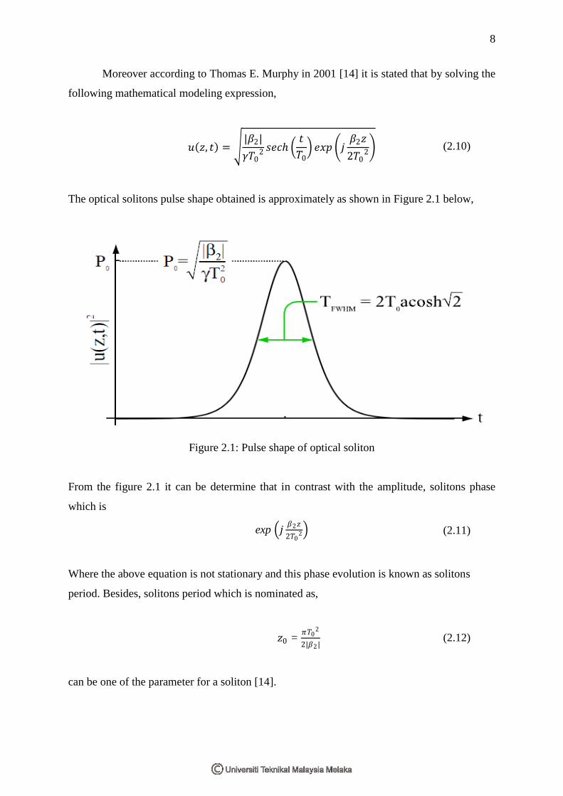
The optical solitons pulse shape obtained is approximately as shown in Figure 2.1 below,
Figure 2.1: Pulse shape of optical soliton
From the figure 2.1 it can be determine that in contrast with the amplitude, solitons phase
which is
exp 𝑗𝛽2𝑧
2𝑇02 (2.11)
Where the above equation is not stationary and this phase evolution is known as solitons
period. Besides, solitons period which is nominated as,
𝑧0 = 𝜋𝑇0
2
2|𝛽2| (2.12)
can be one of the parameter for a soliton [14].

9
2.5 Full Width at Half Maximum
A pulse has an optical power P which is energy per unit time that is substantial only
within some short time intermission and is close to zero at all other times in the time varying
domain. The pulse duration is usually defined as a full width at half maximum (FWHM)
which is the width of the time interval within which the power is as a minimum half the peak
power. The pulse shape of power versus time usually has a rather simple shape, explained for
example with a Gaussian function or a sech2 function, even though complicated pulse shapes
can occur, in instance, as the effect of nonlinear and dispersive distortions, when a pulse
travel through some intermediate [15].
Besides that FWHM could also be defined as a parameter normally used to explain
the distance across of a "bump" on a curve or function. It is given by the length between
points on the curve at which the function reaches half its maximum value [16].

10
CHAPTER 3
OPTICAL SOLITONS SIMULATION
3.1 Overview
From the previous chapter, this chapter will cover on the methodology for this project.
Project methodology is important in order to decide the technique that is to be used in the
project. Besides that, this section will describe the flow of this project. It is an important
criterion that will be implemented in this project. This chapter also will discuss about
procedures that will be use in this project when undergo the simulation of the optical solitons.
3.2 Project Methodology
This project methodology describes the step by step procedure from developing the
optical solitons modeling circuit until the simulation of the optical solitons using both the
optical Gaussian pulse generator and optical sech pulse generator. Besides that this project
methodology will also explained how the optical solitons undergo simulation for both optical
pulse generators at different distances of the nonlinear dispersive fiber total field. Moreover,
this chapter will also portray how the simulation parameters are set up throughout the project
along with the details how the result from the simulation is compared and analysed. The flow
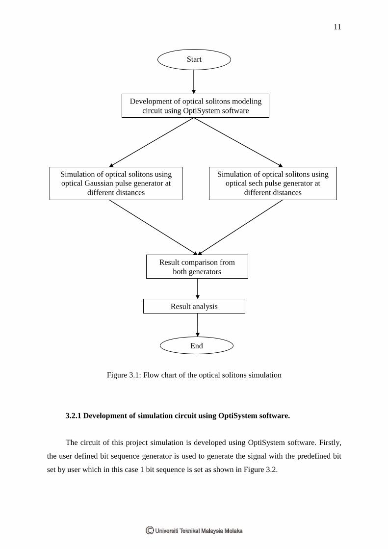
chart in Figure 3.1 illustrated in brief about the step by step procedure of the optical solitons
simulation for single mode optical fiber over 40Gb/s in this project and the Gantt chart of the
project is attached at Appendix A.
11
Start
Development of optical solitons modeling
circuit using OptiSystem software
Simulation of optical solitons using
optical Gaussian pulse generator at
different distances
Simulation of optical solitons using
optical sech pulse generator at
different distances
Result comparison from
both generators
Result analysis
End
Figure 3.1: Flow chart of the optical solitons simulation
3.2.1 Development of simulation circuit using OptiSystem software.
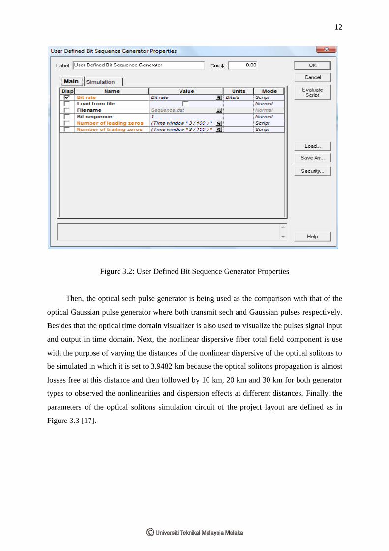
The circuit of this project simulation is developed using OptiSystem software. Firstly,
the user defined bit sequence generator is used to generate the signal with the predefined bit
set by user which in this case 1 bit sequence is set as shown in Figure 3.2.
12
Figure 3.2: User Defined Bit Sequence Generator Properties
Then, the optical sech pulse generator is being used as the comparison with that of the
optical Gaussian pulse generator where both transmit sech and Gaussian pulses respectively.
Besides that the optical time domain visualizer is also used to visualize the pulses signal input
and output in time domain. Next, the nonlinear dispersive fiber total field component is use
with the purpose of varying the distances of the nonlinear dispersive of the optical solitons to
be simulated in which it is set to 3.9482 km because the optical solitons propagation is almost
losses free at this distance and then followed by 10 km, 20 km and 30 km for both generator
types to observed the nonlinearities and dispersion effects at different distances. Finally, the
parameters of the optical solitons simulation circuit of the project layout are defined as in
Figure 3.3 [17].
13
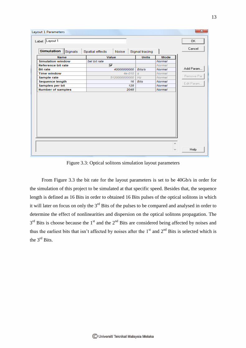
Figure 3.3: Optical solitons simulation layout parameters
From Figure 3.3 the bit rate for the layout parameters is set to be 40Gb/s in order for
the simulation of this project to be simulated at that specific speed. Besides that, the sequence
length is defined as 16 Bits in order to obtained 16 Bits pulses of the optical solitons in which
it will later on focus on only the 3rd
Bits of the pulses to be compared and analysed in order to
determine the effect of nonlinearities and dispersion on the optical solitons propagation. The
3rd
Bits is choose because the 1st and the 2
nd Bits are considered being affected by noises and
thus the earliest bits that isn’t affected by noises after the 1st and 2
nd Bits is selected which is
the 3rd
Bits.
14
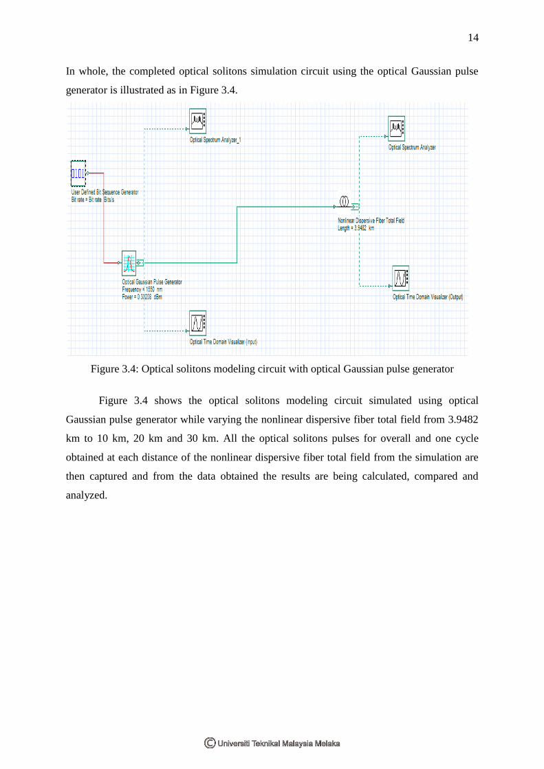
In whole, the completed optical solitons simulation circuit using the optical Gaussian pulse
generator is illustrated as in Figure 3.4.
Figure 3.4: Optical solitons modeling circuit with optical Gaussian pulse generator
Figure 3.4 shows the optical solitons modeling circuit simulated using optical
Gaussian pulse generator while varying the nonlinear dispersive fiber total field from 3.9482
km to 10 km, 20 km and 30 km. All the optical solitons pulses for overall and one cycle
obtained at each distance of the nonlinear dispersive fiber total field from the simulation are
then captured and from the data obtained the results are being calculated, compared and
analyzed.
15
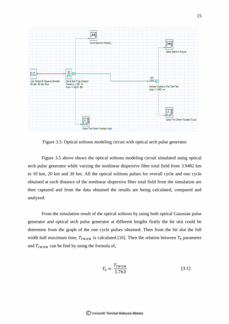
Figure 3.5: Optical solitons modeling circuit with optical sech pulse generator
Figure 3.5 above shows the optical solitons modeling circuit simulated using optical
sech pulse generator while varying the nonlinear dispersive fiber total field from 3.9482 km
to 10 km, 20 km and 30 km. All the optical solitons pulses for overall cycle and one cycle
obtained at each distance of the nonlinear dispersive fiber total field from the simulation are
then captured and from the data obtained the results are being calculated, compared and
analyzed.
From the simulation result of the optical solitons by using both optical Gaussian pulse
generator and optical sech pulse generator at different lengths firstly the bit slot could be
determine from the graph of the one cycle pulses obtained. Then from the bit slot the full
width half maximum time, 𝑇𝐹𝑊𝐻𝑀 is calculated [16]. Then the relation between 𝑇0 parameter
and 𝑇𝐹𝑊𝐻𝑀 can be find by using the formula of,
𝑇0 = 𝑇𝐹𝑊𝐻𝑀
1.763 (3.1)
16
The parameter for the values of nonlinear reference index, 𝑛2 = 2.6 x 10⁻² 𝑚2/ W
and cross-section area of optical fiber 𝐴𝑒𝑓𝑓 = 80 𝜇𝑚2 is used. The power value, 𝑃𝑁 is then
calculated by using the formula of,
𝑃𝑁 = 𝑁2|𝛽2|
𝛾𝑇02 (3.2)
The parameter for the value of the group velocity dispersion, 𝛽2 is set to -20p𝑠2/𝜇𝑚.
Next, the value for the dispersion length, 𝐿𝐷 of the optical soliton pulse is calculated by using
the formula of,
𝐿𝐷 =𝑇0
2
|𝛽2| (3.3)
Later on the solitons period, 𝑍0 is calculated by using the formula of,
𝑍0 =𝜋
2𝐿𝐷 (3.4)
After all the parameter values are obtained and calculated it is then being tabulated in
table at the next chapter and analysed.
17
CHAPTER 4
RESULTS AND DISCUSSIONS
4.0 Data Analysis of Optical Solitons
Based on the optical solitons simulations on previous chapter, the results are recorded
according to the distance of the optical signal travel and also pulses generator used. The detail
results for each of pulses generator used will further analyse and discuss on next section.
4.1 Optical Gaussian Pulse Generator
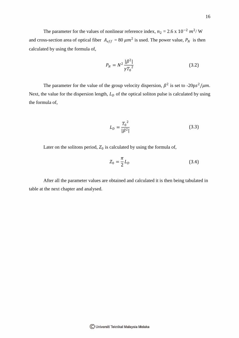
Figure 4.1: Optical solitons overall input propagation before travel over 3.9482 km using
optical Gaussian pulse generator
18
Figure 4.1 shows the overall pulses for input of optical solitons propagation before it travel
for over 3.9482 km of the nonlinear dispersive fiber total field when using optical Gaussian
pulse generator. It shows that the solitons propagation when at the input travels smoothly
without any distortion and preserved its own shape.
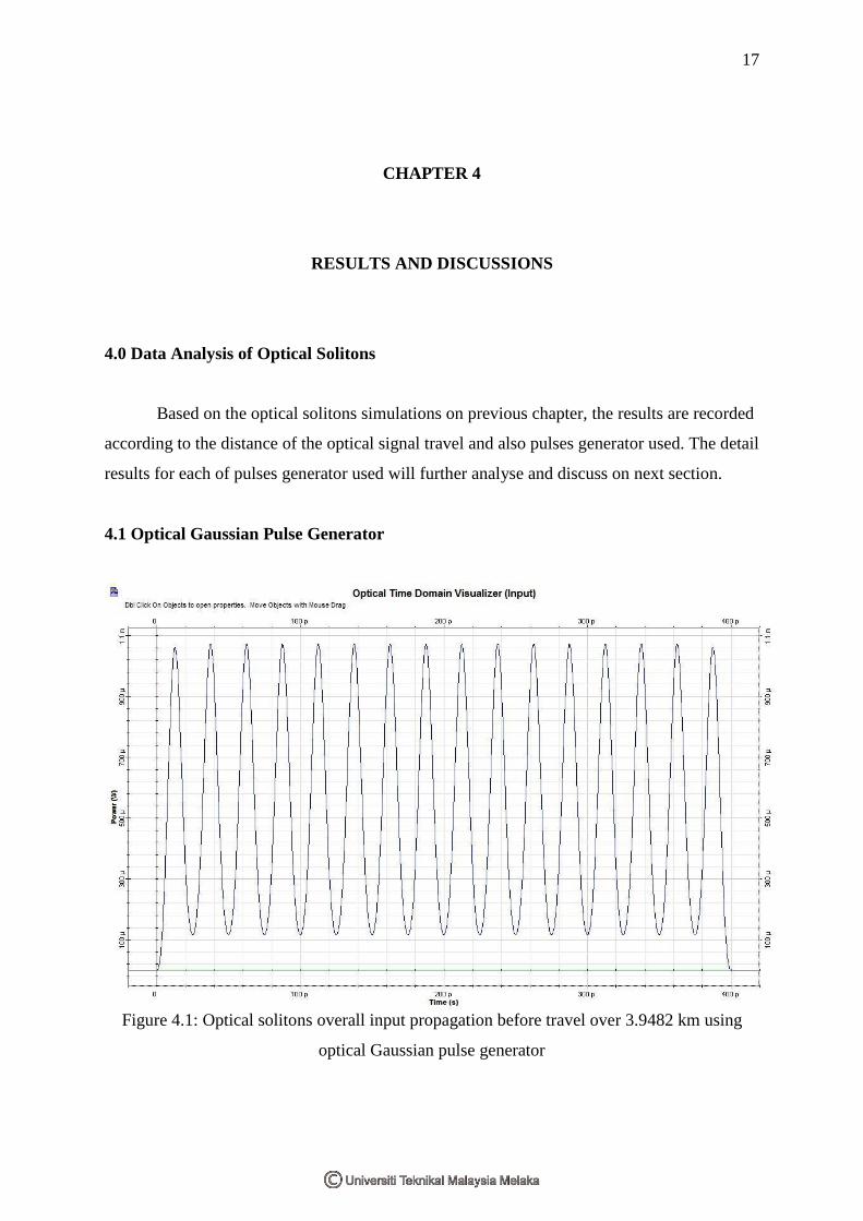
Figure 4.2: Optical solitons one cycle input propagation before travel over 3.9482 km using
optical Gaussian pulse generator
Figure 4.2 shows the one cycle input of optical solitons propagation at the 3rd
bit pulse when
using optical Gaussian pulse generator before it travel at 3.9482 km of the nonlinear
dispersive fiber total field. It can be seen that from the graph, the solitons propagation when
at the input travels smoothly without any distortion and could preserve its own shape. Besides
that, it doesn’t have any overshoots or undershoots. The input peak power at the 3rd
bit pulse
of the optical solitons propagation before travel for 3.9482 km distance is 1071.13𝜇𝑊 that is
obtained from the markers C at y-axis.
19
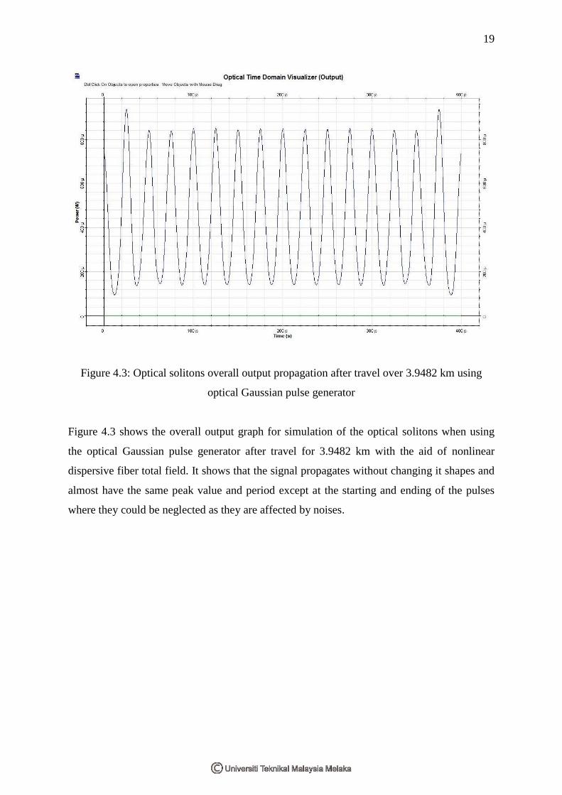
Figure 4.3: Optical solitons overall output propagation after travel over 3.9482 km using
optical Gaussian pulse generator
Figure 4.3 shows the overall output graph for simulation of the optical solitons when using
the optical Gaussian pulse generator after travel for 3.9482 km with the aid of nonlinear
dispersive fiber total field. It shows that the signal propagates without changing it shapes and
almost have the same peak value and period except at the starting and ending of the pulses
where they could be neglected as they are affected by noises.
20
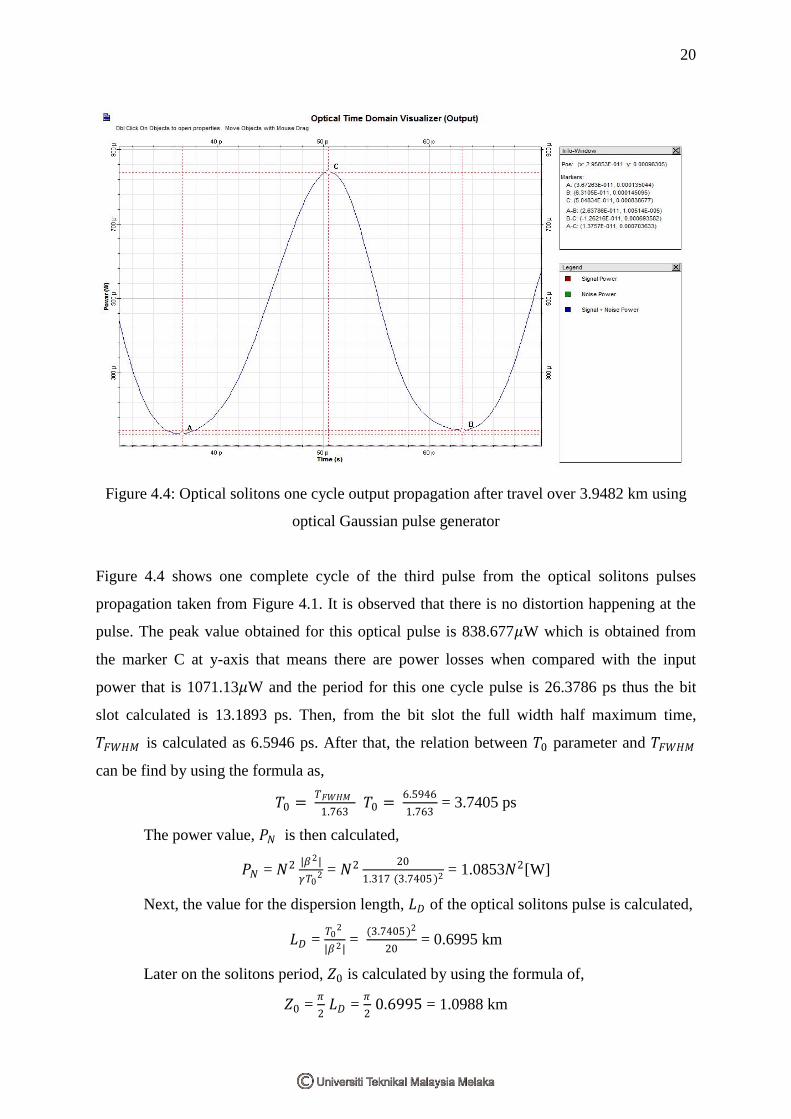
Figure 4.4: Optical solitons one cycle output propagation after travel over 3.9482 km using
optical Gaussian pulse generator
Figure 4.4 shows one complete cycle of the third pulse from the optical solitons pulses
propagation taken from Figure 4.1. It is observed that there is no distortion happening at the
pulse. The peak value obtained for this optical pulse is 838.677𝜇W which is obtained from
the marker C at y-axis that means there are power losses when compared with the input
power that is 1071.13𝜇W and the period for this one cycle pulse is 26.3786 ps thus the bit
slot calculated is 13.1893 ps. Then, from the bit slot the full width half maximum time,
𝑇𝐹𝑊𝐻𝑀 is calculated as 6.5946 ps. After that, the relation between 𝑇0 parameter and 𝑇𝐹𝑊𝐻𝑀
can be find by using the formula as,
𝑇0 = 𝑇𝐹𝑊𝐻𝑀
1.763 𝑇0 =
6.5946
1.763 = 3.7405 ps
The power value, 𝑃𝑁 is then calculated,
𝑃𝑁 = 𝑁2 |𝛽2|
𝛾𝑇02 = 𝑁2 20
1.317 (3.7405 )2 = 1.0853𝑁2[W]
Next, the value for the dispersion length, 𝐿𝐷 of the optical solitons pulse is calculated,
𝐿𝐷 = 𝑇0
2
|𝛽2| =
(3.7405)2
20 = 0.6995 km
Later on the solitons period, 𝑍0 is calculated by using the formula of,
𝑍0 = 𝜋
2 𝐿𝐷 =
𝜋
2 0.6995 = 1.0988 km
21
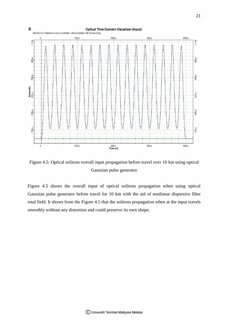
Figure 4.5: Optical solitons overall input propagation before travel over 10 km using optical
Gaussian pulse generator
Figure 4.5 shows the overall input of optical solitons propagation when using optical
Gaussian pulse generator before travel for 10 km with the aid of nonlinear dispersive fiber
total field. It shows from the Figure 4.5 that the solitons propagation when at the input travels
smoothly without any distortion and could preserve its own shape.
22
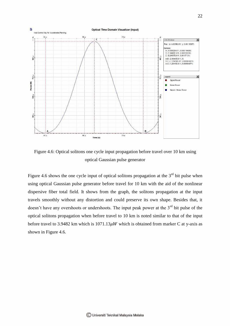
Figure 4.6: Optical solitons one cycle input propagation before travel over 10 km using
optical Gaussian pulse generator
Figure 4.6 shows the one cycle input of optical solitons propagation at the 3rd
bit pulse when
using optical Gaussian pulse generator before travel for 10 km with the aid of the nonlinear
dispersive fiber total field. It shows from the graph, the solitons propagation at the input
travels smoothly without any distortion and could preserve its own shape. Besides that, it
doesn’t have any overshoots or undershoots. The input peak power at the 3rd
bit pulse of the
optical solitons propagation when before travel to 10 km is noted similar to that of the input
before travel to 3.9482 km which is 1071.13𝜇𝑊 which is obtained from marker C at y-axis as
shown in Figure 4.6.
23
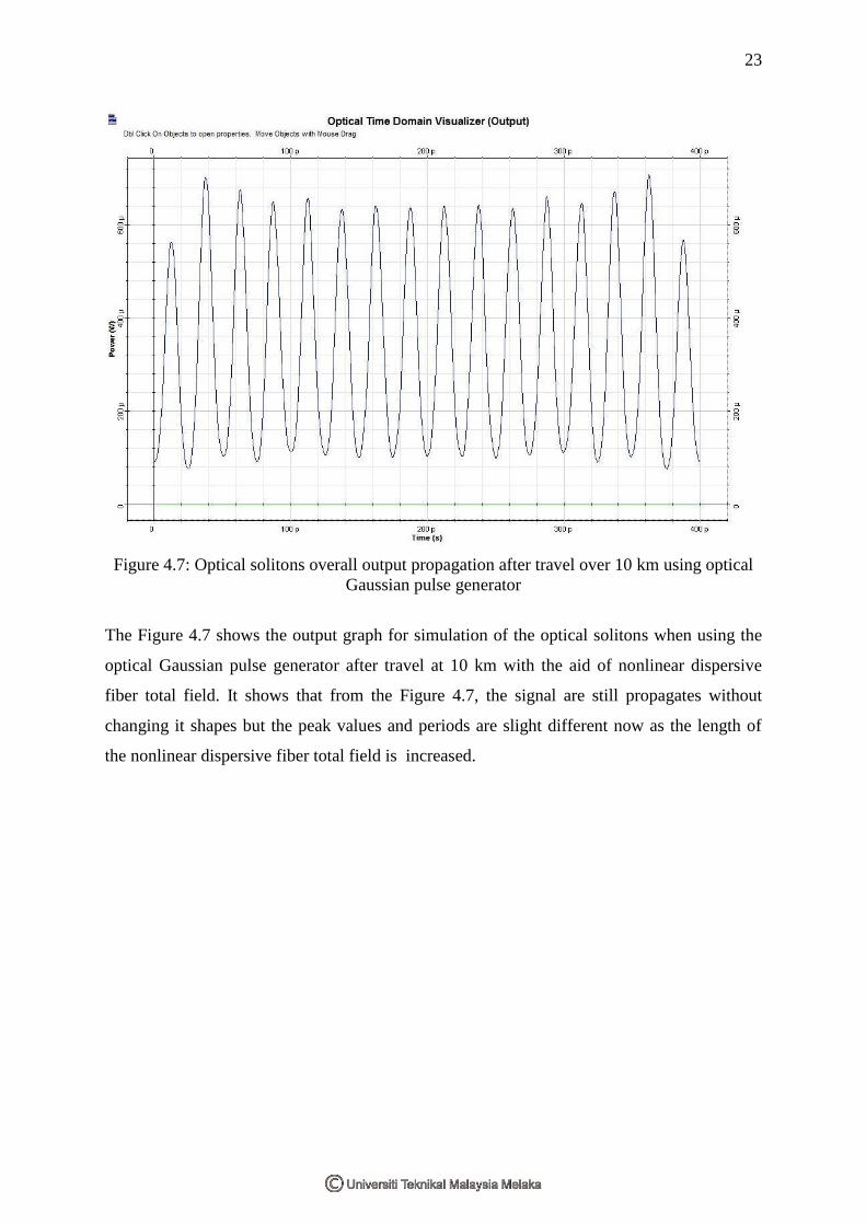
Figure 4.7: Optical solitons overall output propagation after travel over 10 km using optical
Gaussian pulse generator
The Figure 4.7 shows the output graph for simulation of the optical solitons when using the
optical Gaussian pulse generator after travel at 10 km with the aid of nonlinear dispersive
fiber total field. It shows that from the Figure 4.7, the signal are still propagates without
changing it shapes but the peak values and periods are slight different now as the length of
the nonlinear dispersive fiber total field is increased.
24
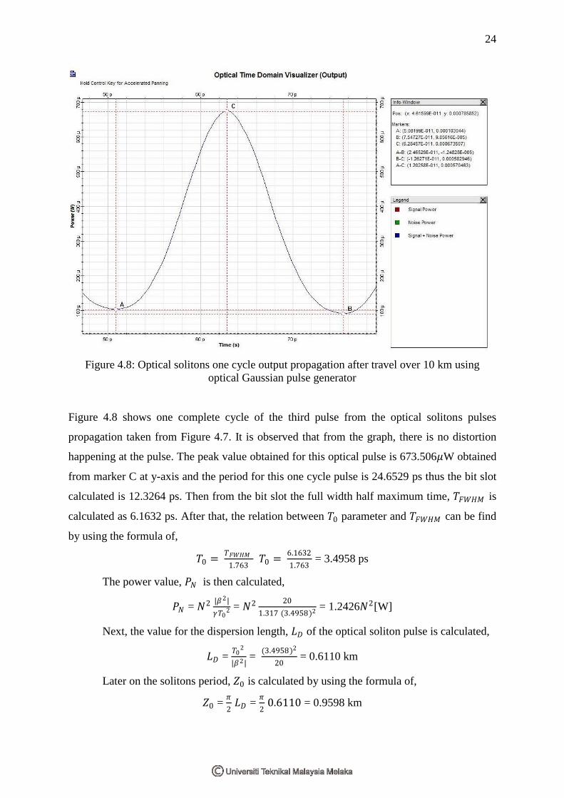
Figure 4.8: Optical solitons one cycle output propagation after travel over 10 km using
optical Gaussian pulse generator
Figure 4.8 shows one complete cycle of the third pulse from the optical solitons pulses
propagation taken from Figure 4.7. It is observed that from the graph, there is no distortion
happening at the pulse. The peak value obtained for this optical pulse is 673.506𝜇W obtained
from marker C at y-axis and the period for this one cycle pulse is 24.6529 ps thus the bit slot
calculated is 12.3264 ps. Then from the bit slot the full width half maximum time, 𝑇𝐹𝑊𝐻𝑀 is
calculated as 6.1632 ps. After that, the relation between 𝑇0 parameter and 𝑇𝐹𝑊𝐻𝑀 can be find
by using the formula of,
𝑇0 = 𝑇𝐹𝑊𝐻𝑀
1.763 𝑇0 =
6.1632
1.763 = 3.4958 ps
The power value, 𝑃𝑁 is then calculated,
𝑃𝑁 = 𝑁2 |𝛽2|
𝛾𝑇02 = 𝑁2 20
1.317 (3.4958)2 = 1.2426𝑁2[W]
Next, the value for the dispersion length, 𝐿𝐷 of the optical soliton pulse is calculated,
𝐿𝐷 = 𝑇0
2
|𝛽2| =
(3.4958)2
20 = 0.6110 km
Later on the solitons period, 𝑍0 is calculated by using the formula of,
𝑍0 = 𝜋
2 𝐿𝐷 =
𝜋
2 0.6110 = 0.9598 km
25
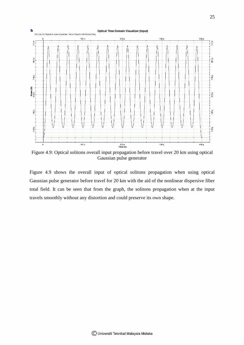
Figure 4.9: Optical solitons overall input propagation before travel over 20 km using optical
Gaussian pulse generator
Figure 4.9 shows the overall input of optical solitons propagation when using optical
Gaussian pulse generator before travel for 20 km with the aid of the nonlinear dispersive fiber
total field. It can be seen that from the graph, the solitons propagation when at the input
travels smoothly without any distortion and could preserve its own shape.
26
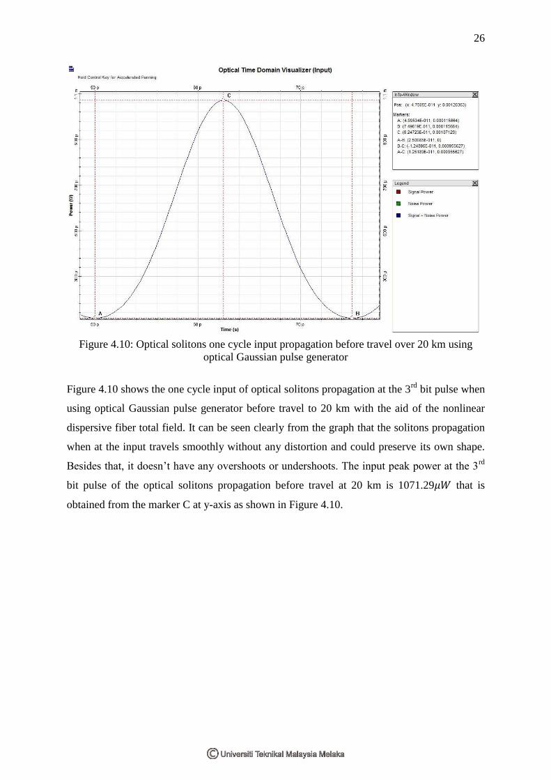
Figure 4.10: Optical solitons one cycle input propagation before travel over 20 km using
optical Gaussian pulse generator
Figure 4.10 shows the one cycle input of optical solitons propagation at the 3rd
bit pulse when
using optical Gaussian pulse generator before travel to 20 km with the aid of the nonlinear
dispersive fiber total field. It can be seen clearly from the graph that the solitons propagation
when at the input travels smoothly without any distortion and could preserve its own shape.
Besides that, it doesn’t have any overshoots or undershoots. The input peak power at the 3rd
bit pulse of the optical solitons propagation before travel at 20 km is 1071.29𝜇𝑊 that is
obtained from the marker C at y-axis as shown in Figure 4.10.
27
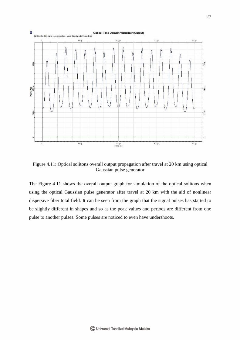
Figure 4.11: Optical solitons overall output propagation after travel at 20 km using optical
Gaussian pulse generator
The Figure 4.11 shows the overall output graph for simulation of the optical solitons when
using the optical Gaussian pulse generator after travel at 20 km with the aid of nonlinear
dispersive fiber total field. It can be seen from the graph that the signal pulses has started to
be slightly different in shapes and so as the peak values and periods are different from one
pulse to another pulses. Some pulses are noticed to even have undershoots.
28
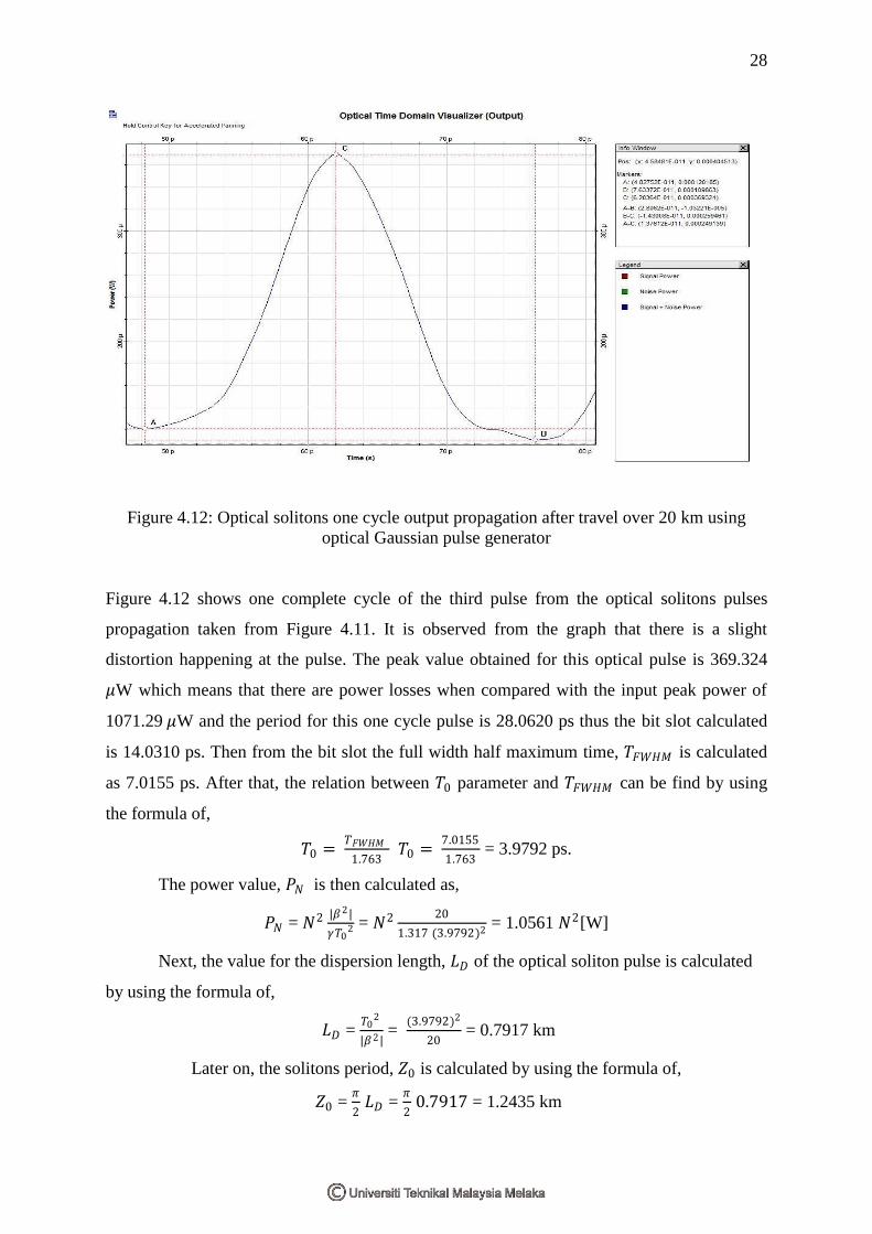
Figure 4.12: Optical solitons one cycle output propagation after travel over 20 km using
optical Gaussian pulse generator
Figure 4.12 shows one complete cycle of the third pulse from the optical solitons pulses
propagation taken from Figure 4.11. It is observed from the graph that there is a slight
distortion happening at the pulse. The peak value obtained for this optical pulse is 369.324
𝜇W which means that there are power losses when compared with the input peak power of
1071.29 𝜇W and the period for this one cycle pulse is 28.0620 ps thus the bit slot calculated
is 14.0310 ps. Then from the bit slot the full width half maximum time, 𝑇𝐹𝑊𝐻𝑀 is calculated
as 7.0155 ps. After that, the relation between 𝑇0 parameter and 𝑇𝐹𝑊𝐻𝑀 can be find by using
the formula of,
𝑇0 = 𝑇𝐹𝑊𝐻𝑀
1.763 𝑇0 =
7.0155
1.763 = 3.9792 ps.
The power value, 𝑃𝑁 is then calculated as,
𝑃𝑁 = 𝑁2 |𝛽2|
𝛾𝑇02 = 𝑁2 20
1.317 (3.9792)2 = 1.0561 𝑁2[W]
Next, the value for the dispersion length, 𝐿𝐷 of the optical soliton pulse is calculated
by using the formula of,
𝐿𝐷 = 𝑇0
2
|𝛽2| =
(3.9792)2
20 = 0.7917 km
Later on, the solitons period, 𝑍0 is calculated by using the formula of,
𝑍0 = 𝜋
2 𝐿𝐷 =
𝜋
2 0.7917 = 1.2435 km
29
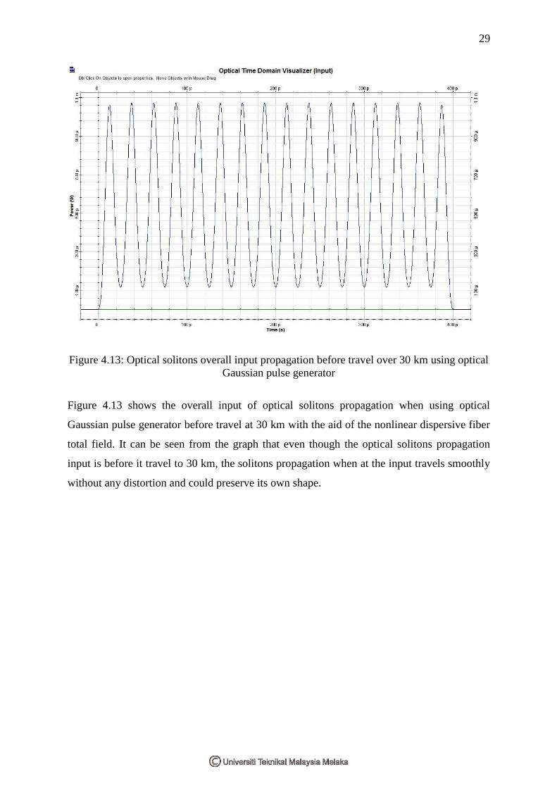
Figure 4.13: Optical solitons overall input propagation before travel over 30 km using optical
Gaussian pulse generator
Figure 4.13 shows the overall input of optical solitons propagation when using optical
Gaussian pulse generator before travel at 30 km with the aid of the nonlinear dispersive fiber
total field. It can be seen from the graph that even though the optical solitons propagation
input is before it travel to 30 km, the solitons propagation when at the input travels smoothly
without any distortion and could preserve its own shape.
30
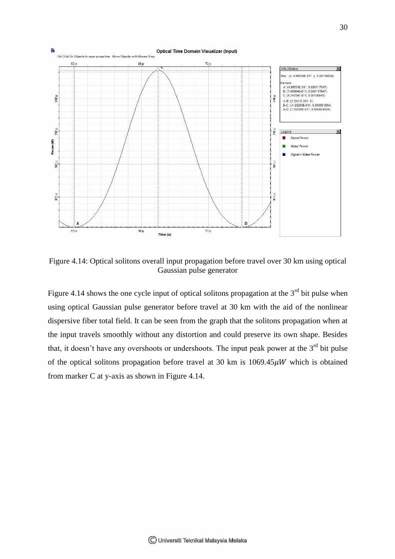
Figure 4.14: Optical solitons overall input propagation before travel over 30 km using optical
Gaussian pulse generator
Figure 4.14 shows the one cycle input of optical solitons propagation at the 3rd
bit pulse when
using optical Gaussian pulse generator before travel at 30 km with the aid of the nonlinear
dispersive fiber total field. It can be seen from the graph that the solitons propagation when at
the input travels smoothly without any distortion and could preserve its own shape. Besides
that, it doesn’t have any overshoots or undershoots. The input peak power at the 3rd
bit pulse
of the optical solitons propagation before travel at 30 km is 1069.45𝜇𝑊 which is obtained
from marker C at y-axis as shown in Figure 4.14.
31
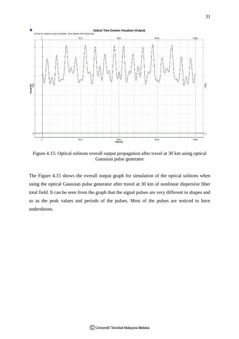
Figure 4.15: Optical solitons overall output propagation after travel at 30 km using optical
Gaussian pulse generator
The Figure 4.15 shows the overall output graph for simulation of the optical solitons when
using the optical Gaussian pulse generator after travel at 30 km of nonlinear dispersive fiber
total field. It can be seen from the graph that the signal pulses are very different in shapes and
so as the peak values and periods of the pulses. Most of the pulses are noticed to have
undershoots.
32
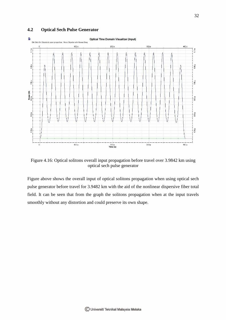
4.2 Optical Sech Pulse Generator
Figure 4.16: Optical solitons overall input propagation before travel over 3.9842 km using
optical sech pulse generator
Figure above shows the overall input of optical solitons propagation when using optical sech
pulse generator before travel for 3.9482 km with the aid of the nonlinear dispersive fiber total
field. It can be seen that from the graph the solitons propagation when at the input travels
smoothly without any distortion and could preserve its own shape.
33
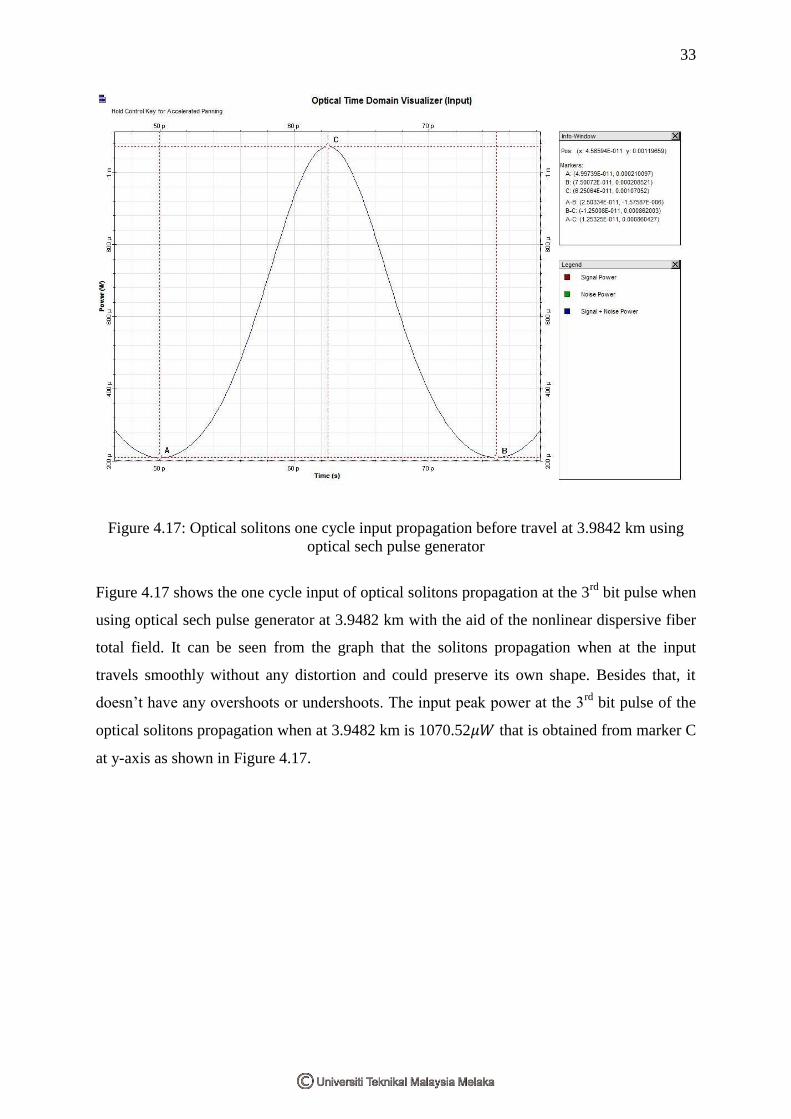
Figure 4.17: Optical solitons one cycle input propagation before travel at 3.9842 km using
optical sech pulse generator
Figure 4.17 shows the one cycle input of optical solitons propagation at the 3rd
bit pulse when
using optical sech pulse generator at 3.9482 km with the aid of the nonlinear dispersive fiber
total field. It can be seen from the graph that the solitons propagation when at the input
travels smoothly without any distortion and could preserve its own shape. Besides that, it
doesn’t have any overshoots or undershoots. The input peak power at the 3rd
bit pulse of the
optical solitons propagation when at 3.9482 km is 1070.52𝜇𝑊 that is obtained from marker C
at y-axis as shown in Figure 4.17.
34
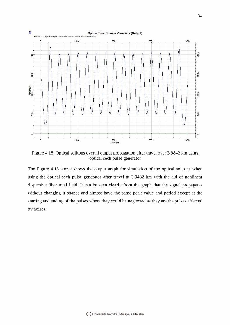
Figure 4.18: Optical solitons overall output propagation after travel over 3.9842 km using
optical sech pulse generator
The Figure 4.18 above shows the output graph for simulation of the optical solitons when
using the optical sech pulse generator after travel at 3.9482 km with the aid of nonlinear
dispersive fiber total field. It can be seen clearly from the graph that the signal propagates
without changing it shapes and almost have the same peak value and period except at the
starting and ending of the pulses where they could be neglected as they are the pulses affected
by noises.
35
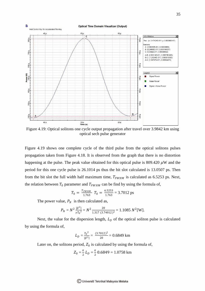
Figure 4.19: Optical solitons one cycle output propagation after travel over 3.9842 km using
optical sech pulse generator
Figure 4.19 shows one complete cycle of the third pulse from the optical solitons pulses
propagation taken from Figure 4.18. It is observed from the graph that there is no distortion
happening at the pulse. The peak value obtained for this optical pulse is 809.420 𝜇W and the
period for this one cycle pulse is 26.1014 ps thus the bit slot calculated is 13.0507 ps. Then
from the bit slot the full width half maximum time, 𝑇𝐹𝑊𝐻𝑀 is calculated as 6.5253 ps. Next,
the relation between 𝑇0 parameter and 𝑇𝐹𝑊𝐻𝑀 can be find by using the formula of,
𝑇0 = 𝑇𝐹𝑊𝐻𝑀
1.763 𝑇0 =
6.5253
1.763 = 3.7012 ps
The power value, 𝑃𝑁 is then calculated as,
𝑃𝑁 = 𝑁2 |𝛽2|
𝛾𝑇02 = 𝑁2 20
1.317 (3.74012 )2 = 1.1085 𝑁2[W].
Next, the value for the dispersion length, 𝐿𝐷 of the optical soliton pulse is calculated
by using the formula of,
𝐿𝐷 = 𝑇0
2
|𝛽2| =
(3.7012)2
20 = 0.6849 km
Later on, the solitons period, 𝑍0 is calculated by using the formula of,
𝑍0 = 𝜋
2 𝐿𝐷 =
𝜋
2 0.6849 = 1.0758 km
36
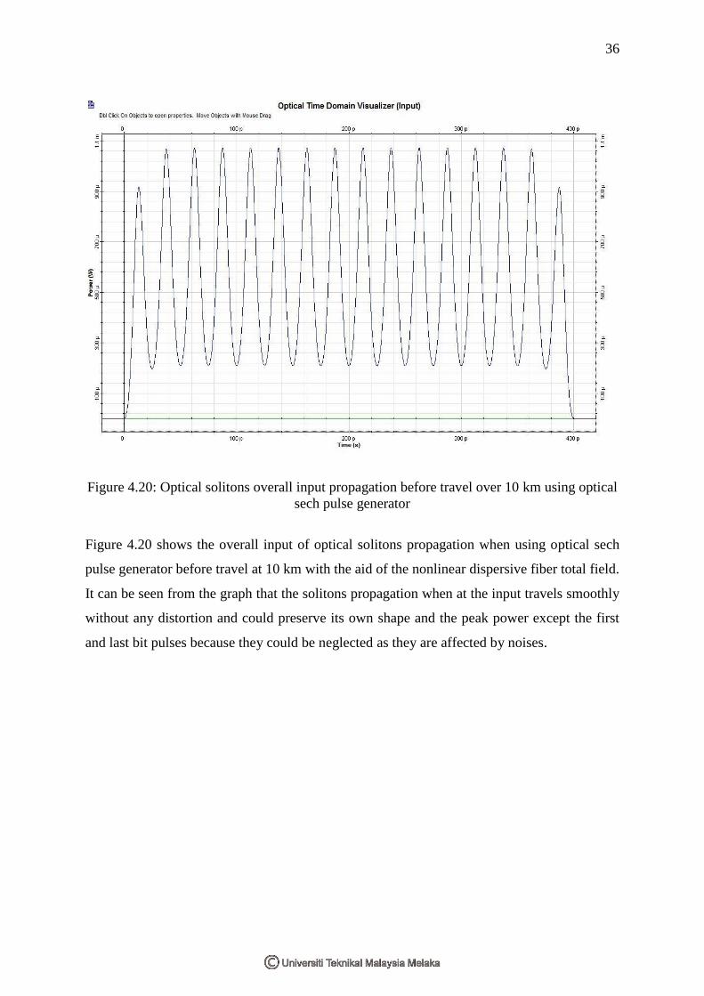
Figure 4.20: Optical solitons overall input propagation before travel over 10 km using optical
sech pulse generator
Figure 4.20 shows the overall input of optical solitons propagation when using optical sech
pulse generator before travel at 10 km with the aid of the nonlinear dispersive fiber total field.
It can be seen from the graph that the solitons propagation when at the input travels smoothly
without any distortion and could preserve its own shape and the peak power except the first
and last bit pulses because they could be neglected as they are affected by noises.
37
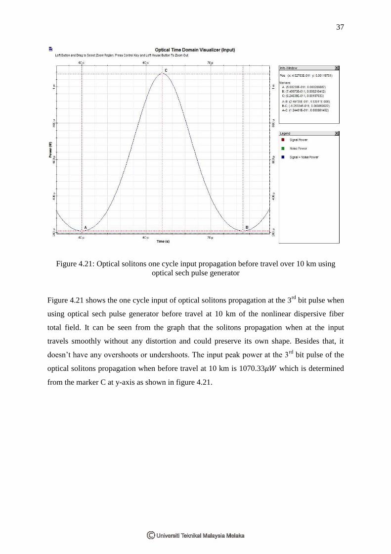
Figure 4.21: Optical solitons one cycle input propagation before travel over 10 km using
optical sech pulse generator
Figure 4.21 shows the one cycle input of optical solitons propagation at the 3rd
bit pulse when
using optical sech pulse generator before travel at 10 km of the nonlinear dispersive fiber
total field. It can be seen from the graph that the solitons propagation when at the input
travels smoothly without any distortion and could preserve its own shape. Besides that, it
doesn’t have any overshoots or undershoots. The input peak power at the 3rd
bit pulse of the
optical solitons propagation when before travel at 10 km is 1070.33𝜇𝑊 which is determined
from the marker C at y-axis as shown in figure 4.21.
38
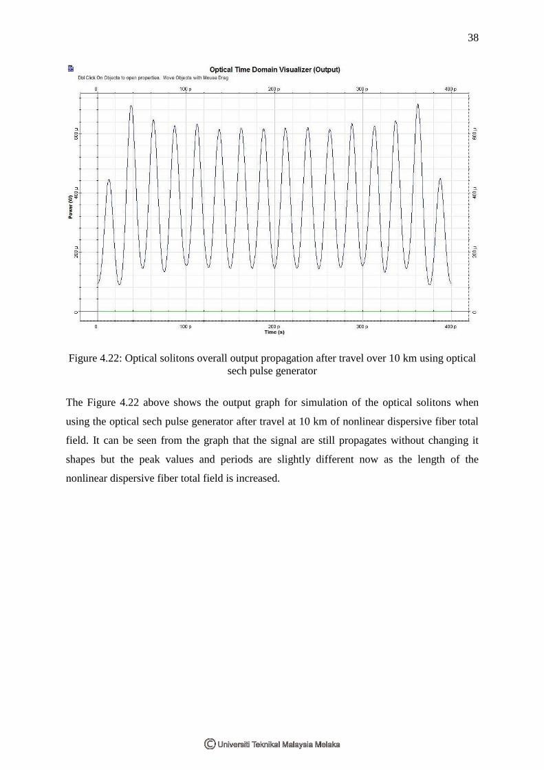
Figure 4.22: Optical solitons overall output propagation after travel over 10 km using optical
sech pulse generator
The Figure 4.22 above shows the output graph for simulation of the optical solitons when
using the optical sech pulse generator after travel at 10 km of nonlinear dispersive fiber total
field. It can be seen from the graph that the signal are still propagates without changing it
shapes but the peak values and periods are slightly different now as the length of the
nonlinear dispersive fiber total field is increased.
39
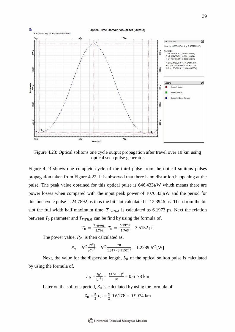
Figure 4.23: Optical solitons one cycle output propagation after travel over 10 km using
optical sech pulse generator
Figure 4.23 shows one complete cycle of the third pulse from the optical solitons pulses
propagation taken from Figure 4.22. It is observed that there is no distortion happening at the
pulse. The peak value obtained for this optical pulse is 646.433𝜇W which means there are
power losses when compared with the input peak power of 1070.33 𝜇W and the period for
this one cycle pulse is 24.7892 ps thus the bit slot calculated is 12.3946 ps. Then from the bit
slot the full width half maximum time, 𝑇𝐹𝑊𝐻𝑀 is calculated as 6.1973 ps. Next the relation
between 𝑇0 parameter and 𝑇𝐹𝑊𝐻𝑀 can be find by using the formula of,
𝑇0 = 𝑇𝐹𝑊𝐻𝑀
1.763 𝑇0 =
6.1973
1.763 = 3.5152 ps
The power value, 𝑃𝑁 is then calculated as,
𝑃𝑁 = 𝑁2 |𝛽2|
𝛾𝑇02 = 𝑁2 20
1.317 (3.5152 )2 = 1.2289 𝑁2[W]
Next, the value for the dispersion length, 𝐿𝐷 of the optical soliton pulse is calculated
by using the formula of,
𝐿𝐷 = 𝑇0
2
|𝛽2| =
(3.5152)2
20 = 0.6178 km
Later on the solitons period, 𝑍0 is calculated by using the formula of,
𝑍0 = 𝜋
2 𝐿𝐷 =
𝜋
2 0.6178 = 0.9074 km
40
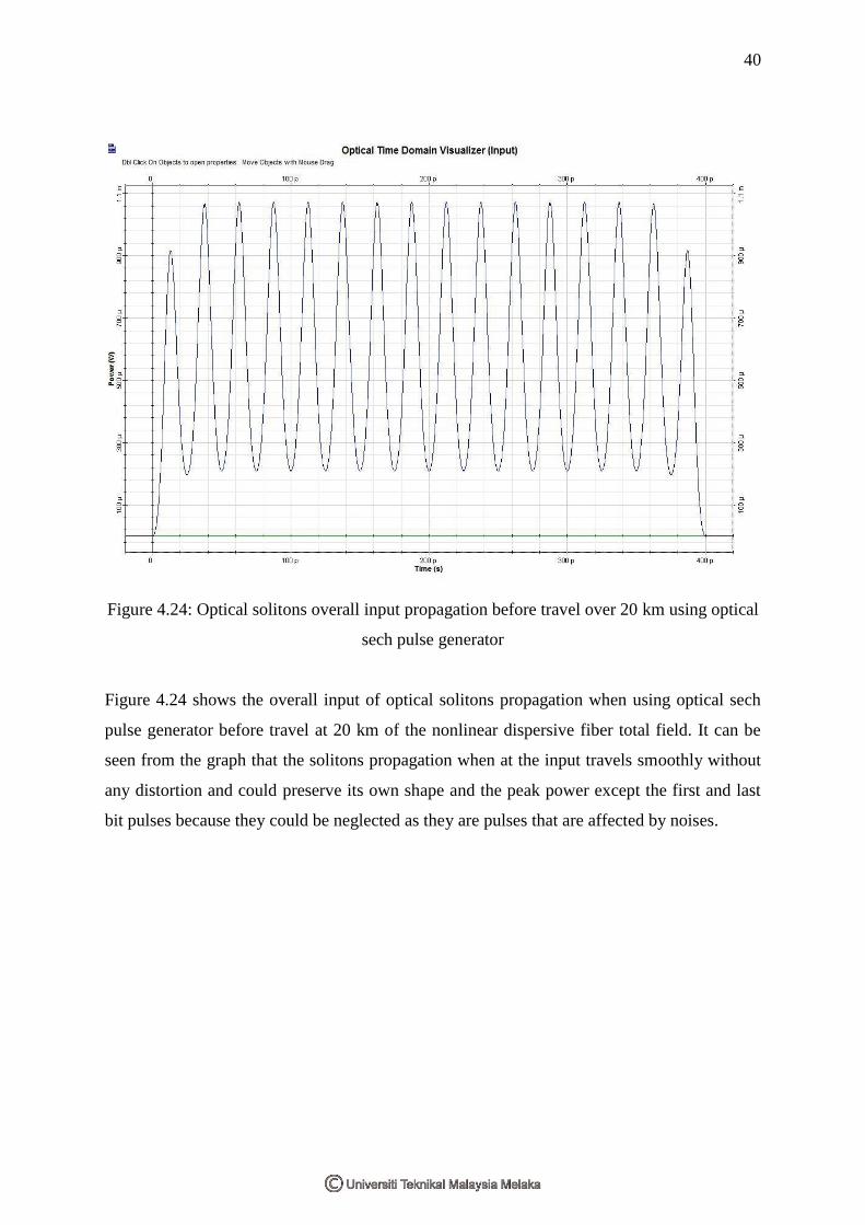
Figure 4.24: Optical solitons overall input propagation before travel over 20 km using optical
sech pulse generator
Figure 4.24 shows the overall input of optical solitons propagation when using optical sech
pulse generator before travel at 20 km of the nonlinear dispersive fiber total field. It can be
seen from the graph that the solitons propagation when at the input travels smoothly without
any distortion and could preserve its own shape and the peak power except the first and last
bit pulses because they could be neglected as they are pulses that are affected by noises.
41
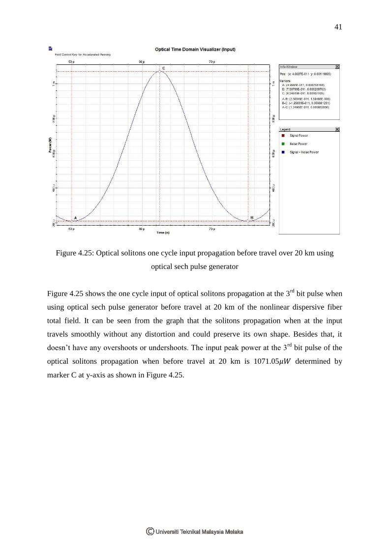
Figure 4.25: Optical solitons one cycle input propagation before travel over 20 km using
optical sech pulse generator
Figure 4.25 shows the one cycle input of optical solitons propagation at the 3rd
bit pulse when
using optical sech pulse generator before travel at 20 km of the nonlinear dispersive fiber
total field. It can be seen from the graph that the solitons propagation when at the input
travels smoothly without any distortion and could preserve its own shape. Besides that, it
doesn’t have any overshoots or undershoots. The input peak power at the 3rd
bit pulse of the
optical solitons propagation when before travel at 20 km is 1071.05𝜇𝑊 determined by
marker C at y-axis as shown in Figure 4.25.
42
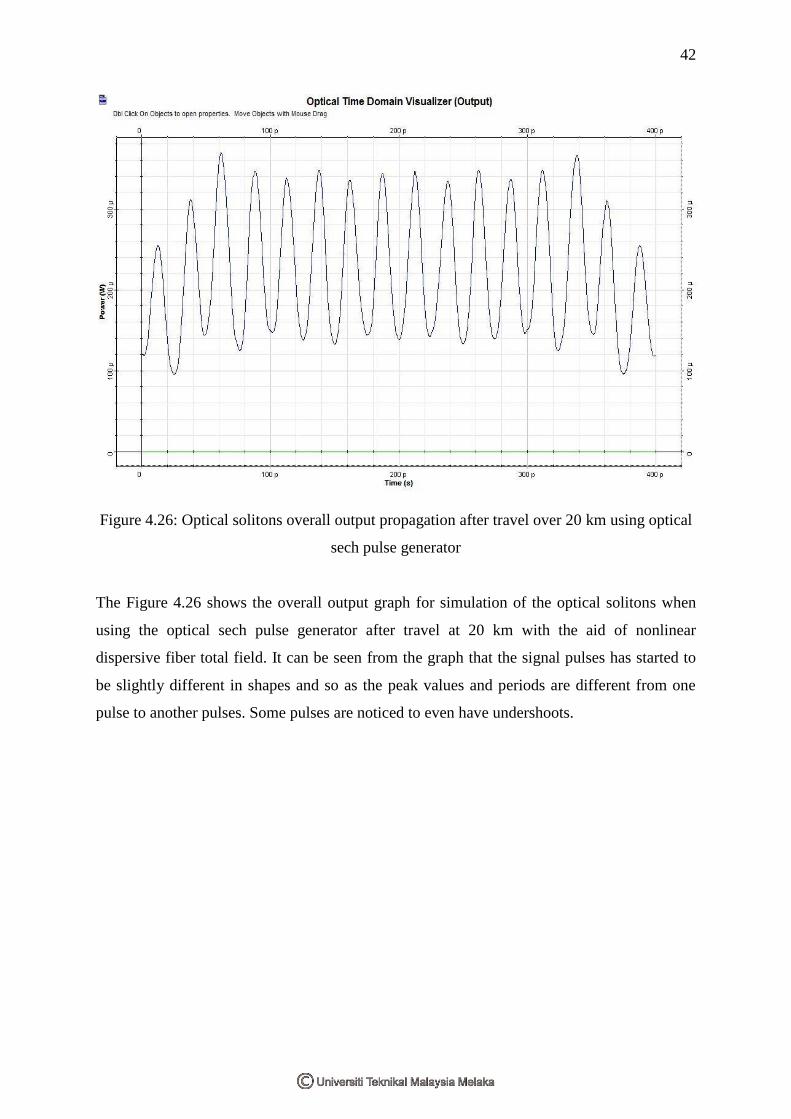
Figure 4.26: Optical solitons overall output propagation after travel over 20 km using optical
sech pulse generator
The Figure 4.26 shows the overall output graph for simulation of the optical solitons when
using the optical sech pulse generator after travel at 20 km with the aid of nonlinear
dispersive fiber total field. It can be seen from the graph that the signal pulses has started to
be slightly different in shapes and so as the peak values and periods are different from one
pulse to another pulses. Some pulses are noticed to even have undershoots.
43
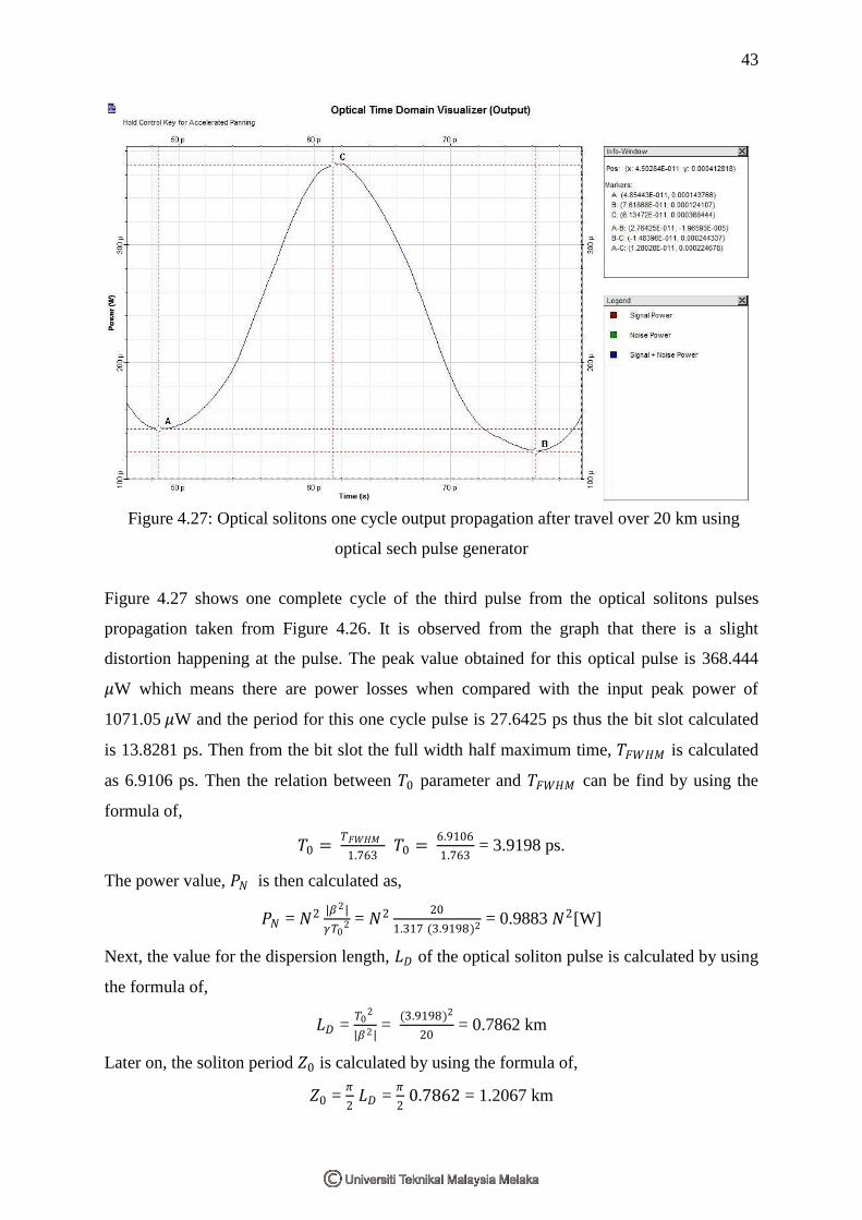
Figure 4.27: Optical solitons one cycle output propagation after travel over 20 km using
optical sech pulse generator
Figure 4.27 shows one complete cycle of the third pulse from the optical solitons pulses
propagation taken from Figure 4.26. It is observed from the graph that there is a slight
distortion happening at the pulse. The peak value obtained for this optical pulse is 368.444
𝜇W which means there are power losses when compared with the input peak power of
1071.05 𝜇W and the period for this one cycle pulse is 27.6425 ps thus the bit slot calculated
is 13.8281 ps. Then from the bit slot the full width half maximum time, 𝑇𝐹𝑊𝐻𝑀 is calculated
as 6.9106 ps. Then the relation between 𝑇0 parameter and 𝑇𝐹𝑊𝐻𝑀 can be find by using the
formula of,
𝑇0 = 𝑇𝐹𝑊𝐻𝑀
1.763 𝑇0 =
6.9106
1.763 = 3.9198 ps.
The power value, 𝑃𝑁 is then calculated as,
𝑃𝑁 = 𝑁2 |𝛽2|
𝛾𝑇02 = 𝑁2 20
1.317 (3.9198)2 = 0.9883 𝑁2[W]
Next, the value for the dispersion length, 𝐿𝐷 of the optical soliton pulse is calculated by using
the formula of,
𝐿𝐷 = 𝑇0
2
|𝛽2| =
(3.9198)2
20 = 0.7862 km
Later on, the soliton period 𝑍0 is calculated by using the formula of,
𝑍0 = 𝜋
2 𝐿𝐷 =
𝜋
2 0.7862 = 1.2067 km
44
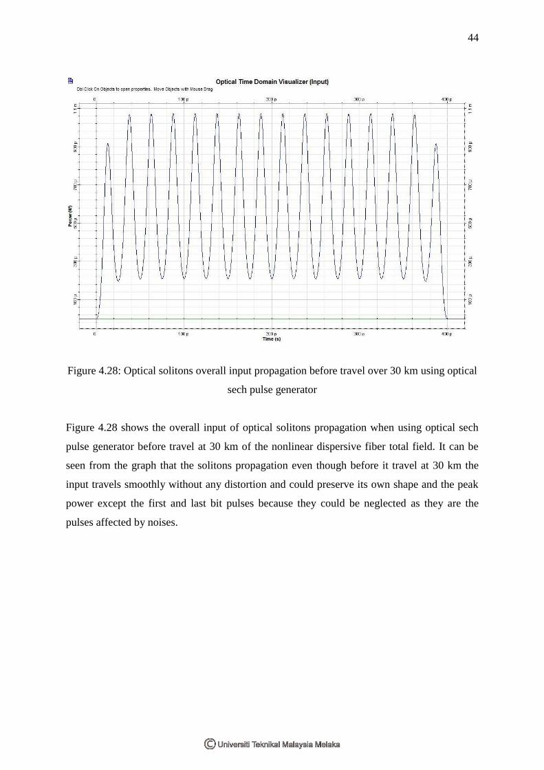
Figure 4.28: Optical solitons overall input propagation before travel over 30 km using optical
sech pulse generator
Figure 4.28 shows the overall input of optical solitons propagation when using optical sech
pulse generator before travel at 30 km of the nonlinear dispersive fiber total field. It can be
seen from the graph that the solitons propagation even though before it travel at 30 km the
input travels smoothly without any distortion and could preserve its own shape and the peak
power except the first and last bit pulses because they could be neglected as they are the
pulses affected by noises.
45
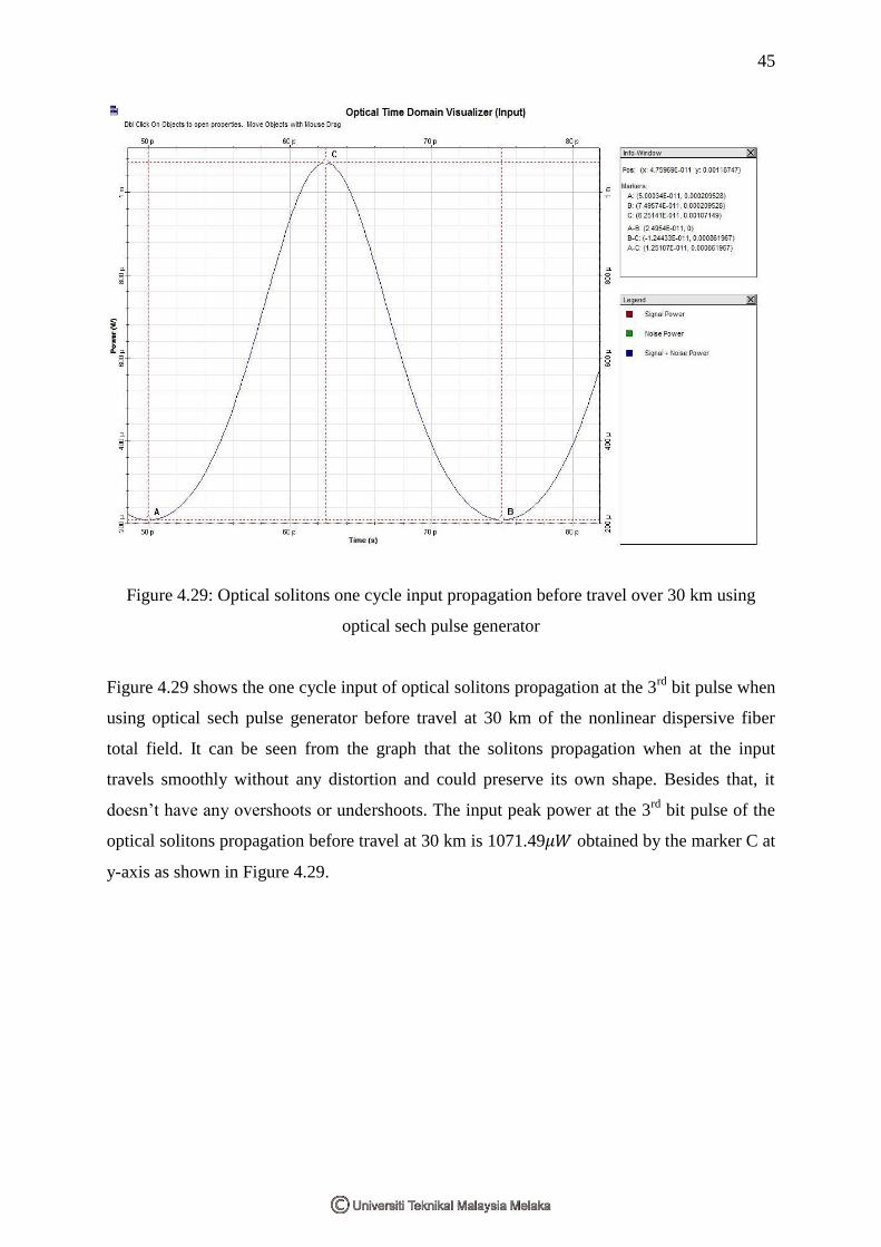
Figure 4.29: Optical solitons one cycle input propagation before travel over 30 km using
optical sech pulse generator
Figure 4.29 shows the one cycle input of optical solitons propagation at the 3rd
bit pulse when
using optical sech pulse generator before travel at 30 km of the nonlinear dispersive fiber
total field. It can be seen from the graph that the solitons propagation when at the input
travels smoothly without any distortion and could preserve its own shape. Besides that, it
doesn’t have any overshoots or undershoots. The input peak power at the 3rd
bit pulse of the
optical solitons propagation before travel at 30 km is 1071.49𝜇𝑊 obtained by the marker C at
y-axis as shown in Figure 4.29.
46
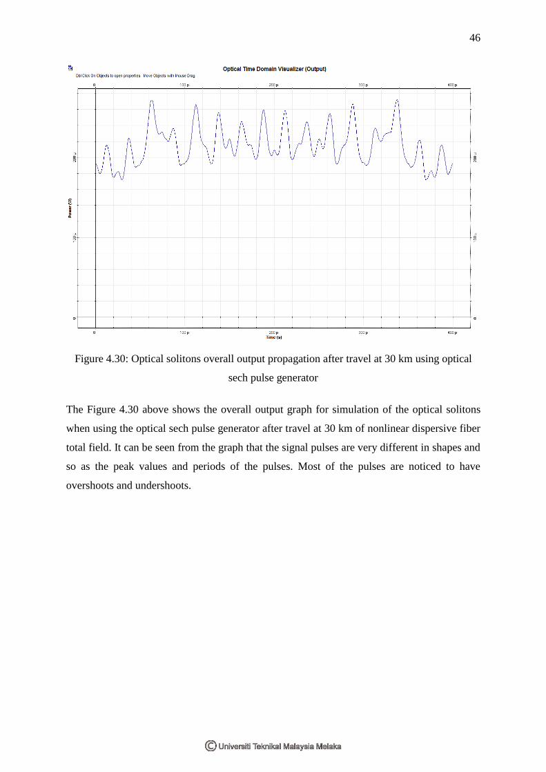
Figure 4.30: Optical solitons overall output propagation after travel at 30 km using optical
sech pulse generator
The Figure 4.30 above shows the overall output graph for simulation of the optical solitons
when using the optical sech pulse generator after travel at 30 km of nonlinear dispersive fiber
total field. It can be seen from the graph that the signal pulses are very different in shapes and
so as the peak values and periods of the pulses. Most of the pulses are noticed to have
overshoots and undershoots.

47
From the output of the simulations obtained, the results for the Gaussian pulse and sech pulse
could be compared in the table below:
Table 4.1: Comparison of the sech signal and Gaussian Signal on simulation model
Distance Gaussian Pulse Sech Pulse
3.9482k
m
10km
20km
30km
From the signals in Table 4.1 it is observed that the optical solitons signal when travel over
3.9482 km and 10 km distances either using sech or Gaussian pulse they propagate without
48
changing their shape and even propagate at almost the same peak power undistorted. But then
the optical solitons signal started to differ slightly in shape and peak power when they travel
over 20 km be it with the sech or Gaussian pulse. However when the optical solitons signal
travel at 30 km the signals are could no longer preserve their shape and peak power and at
this rate they have overshoots and undershoots.
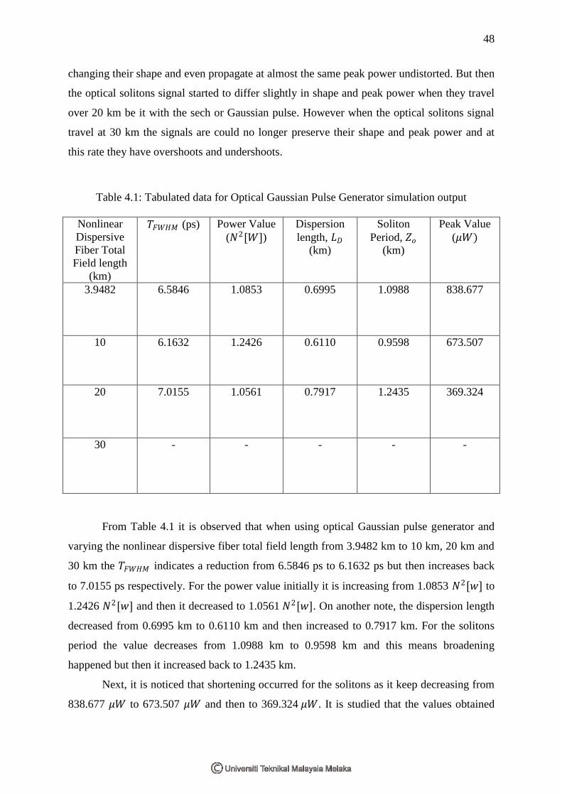
Table 4.1: Tabulated data for Optical Gaussian Pulse Generator simulation output
Nonlinear
Dispersive
Fiber Total
Field length
(km)
𝑇𝐹𝑊𝐻𝑀 (ps) Power Value
(𝑁2[𝑊]) Dispersion
length, 𝐿𝐷
(km)
Soliton
Period, 𝑍𝑜
(km)
Peak Value
(𝜇𝑊)
3.9482 6.5846 1.0853 0.6995 1.0988 838.677
10 6.1632 1.2426 0.6110 0.9598 673.507
20 7.0155 1.0561 0.7917 1.2435 369.324
30 - - - - -
From Table 4.1 it is observed that when using optical Gaussian pulse generator and
varying the nonlinear dispersive fiber total field length from 3.9482 km to 10 km, 20 km and
30 km the 𝑇𝐹𝑊𝐻𝑀 indicates a reduction from 6.5846 ps to 6.1632 ps but then increases back
to 7.0155 ps respectively. For the power value initially it is increasing from 1.0853 𝑁2[𝑤] to
1.2426 𝑁2[𝑤] and then it decreased to 1.0561 𝑁2[𝑤]. On another note, the dispersion length
decreased from 0.6995 km to 0.6110 km and then increased to 0.7917 km. For the solitons
period the value decreases from 1.0988 km to 0.9598 km and this means broadening
happened but then it increased back to 1.2435 km.
Next, it is noticed that shortening occurred for the solitons as it keep decreasing from
838.677 𝜇𝑊 to 673.507 𝜇𝑊 and then to 369.324 𝜇𝑊. It is studied that the values obtained
49
excluding peak values didn’t show any fixed pattern and they are either increased at first and
then decreased or initially decreased and then increased because of the nonlinearities in
optical soliton. When at 30 km, all the values for parameters𝑇𝐹𝑊𝐻𝑀 , power value, dispersion
length and soliton period couldn’t be traced because the output bit slot couldn’t be
determined.
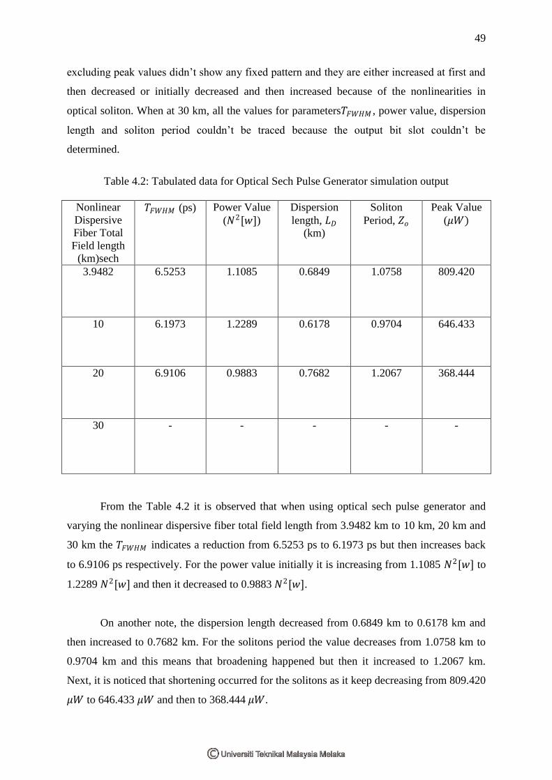
Table 4.2: Tabulated data for Optical Sech Pulse Generator simulation output
Nonlinear
Dispersive
Fiber Total
Field length
(km)sech
𝑇𝐹𝑊𝐻𝑀 (ps) Power Value
(𝑁2[𝑤]) Dispersion
length, 𝐿𝐷
(km)
Soliton
Period, 𝑍𝑜
Peak Value
(𝜇𝑊)
3.9482 6.5253 1.1085 0.6849 1.0758 809.420
10 6.1973 1.2289 0.6178 0.9704 646.433
20 6.9106 0.9883 0.7682 1.2067 368.444
30 - - - - -
From the Table 4.2 it is observed that when using optical sech pulse generator and
varying the nonlinear dispersive fiber total field length from 3.9482 km to 10 km, 20 km and
30 km the 𝑇𝐹𝑊𝐻𝑀 indicates a reduction from 6.5253 ps to 6.1973 ps but then increases back
to 6.9106 ps respectively. For the power value initially it is increasing from 1.1085 𝑁2[𝑤] to
1.2289 𝑁2[𝑤] and then it decreased to 0.9883 𝑁2[𝑤].
On another note, the dispersion length decreased from 0.6849 km to 0.6178 km and
then increased to 0.7682 km. For the solitons period the value decreases from 1.0758 km to
0.9704 km and this means that broadening happened but then it increased to 1.2067 km.
Next, it is noticed that shortening occurred for the solitons as it keep decreasing from 809.420
𝜇𝑊 to 646.433 𝜇𝑊 and then to 368.444 𝜇𝑊.
50
It is studied that the values obtained excluding the peak value didn’t show any fixed
pattern and they are either increased at first and then decreased or initially decreased and then
increased because of the nonlinearities in optical solitons. However it shows similarity with
that of the optical Gaussian pulse generator in terms of increasing and decreasing of the
parameter values.
When at 30 km, all the values for parameters 𝑇𝐹𝑊𝐻𝑀 , power value, dispersion length
and soliton period couldn’t be traced because the output bit slot couldn’t be determined. At
this distance it is obvious that the optical solitons couldn’t preserve its own shape anymore. It
is also observed that pulses shape obtained for both optical Gaussian pulse generator and
optical sech pulse generator is similar to the one expected from the literature review [13].
Besides that, it is also examined that the dispersion length obtained for optical solitons
propagation output when using optical Gaussian pulse generator is higher than that of the
optical sech pulse generator and when relate to communication system optical solitons that
have higher dispersion length will results in higher data losses due to the scattering effect.
Other than that, it is also observed during the simulation that when comparing the
input and the output peak power of the optical solitons propagation there are power losses
occurred for each simulation process either the optical Gaussian pulse generator or optical
sech pulse generator is used at any distances. This is most probably because of the
imperfection of the optical fiber.
4.3 Result and Discussion Summary
From the results and discussion in the previous section it is studied that the optical
solitons propagation formed due to the simulation are as predicted as in the literature review.
On another note, it is also determined that when using optical sech pulse generator data losses
could be reduced due to the scattering effect since it have lower dispersion length when
compared with the Gaussian pulse. Besides that the nonlinearity effect of the optical solitons
are observed when varying the distances of the nonlinear dispersive fiber total field especially
when the parameter values obtained are either initially increased and then decreased back or
initially decreased and then increased back. Moreover, the power losses from the input to the
output peak power of the optical solitons are also identified due to the imperfection of the
optical fiber.
51
CHAPTER 5
CONCLUSION AND RECOMMENDATIONS
5.1 Conclusion
As the conclusion, optical solitons could be modeled and simulated by using
OptiSytem software whether by using optical Gaussian pulse generator or optical sech pulse
generator. Moreover, it could be said that based on the analysis it is better to use optical sech
pulse generator compared to optical Gaussian pulse generator as it have lower dispersion
length and thus have lower losses in communication system due to the scattering effects.
From the simulation the effects of nonlinearity and dispersion are able to be observed due to
the shortening and broadening of the optical pulses. Besides that, the use of nonlinear
dispersive fiber total field is successfully implemented in this project. This is because by
controlling the distance of the nonlinear dispersive fiber total field, the dispersion length and
the soliton period could also be control. Last but not least, from this project it is proved that
the theoretical aspect and simulation result about the effects of nonlinearity is existed in
optical solitons where the result can be compare through theory and simulation.
5.2 Recommendations
The optical solitons simulation could always have a space for improvement, and this
project is also included. Since there are still lacks of practical use in optical solitons, a few
recommendations had been carried out in order to have more alternatives ways in learning
process. These recommendations are based on attractive learning and also observation from
the project. Here are some suggestions for the future development;
Simulation of optical solitons in single mode optical fiber for over 40Gb/s with the
use of multiplexer

52
Optical solitons simulation in multimode optical fiber for over 40Gb/s
Implementation of the simulation of the optical solitons in single mode optical fiber
(Hardware implementation)
5.3 Project Potential
In communication systems, this project has a potential for being used. This is because
this project improvises the speed of the communication system through optical fiber and the
optical fiber for communication systems are currently in demand as it is being used for
internet connection, phone telecommunication and even internet protocol television. Besides,
this project also can produce lower losses and provides stability to the communication
system.
53
REFERENCES
[1] Y. S., Kivshar and G.P., Agrawal, Optical solitons: From Fibers to Photonic Crystals,
Academic Press, 2003,pp1-2
[2] J. S., Russell, Report of 14th Meeting of the British Association for Advancement of
Science, York, September 1844, pp. 311-390.
[3] M. J., Ablowitz and P. A. Clarkson, Solitons, Nonlinear Evolution Equations, and Inverse
Scattering, New York,: Cambridge University Press, 1991
[4] C. S., Gardner, J. M., Green, M. D.. Kruskal, and R. M., Miura, Phys. Rev. Lett. 19, 1095
(1967); Commun. Pure Appl. Math. 27, 97 (1974).
[5] Y., R., Shen, Principles of Nonlinear Optics, New York: Wiley, 1984.
[6] P. N., Butcher and D. N., Cotter, The Elements of Nonlinear Optics. Cambridge
University Press:UK, 1990.
[7] R.W., Boyd, Nonlinear Optics, San Diego: Academic Press, 1992
[8] G. P., Agrawal, Nonlinear Fiber Optics, 3rd ed.. San Diego, Academic Press, 2001
[9] A., Hasegawa and E., Tappert, Appl. Phys. Lett. 23, 171 (1973).
[10] R. Y., Chiao, E., Garmire, and C. H., Townes, Phys. Rev. Lett. 13, 479 (1964).
[11] A., Hasegawa and E., Tappert, Appl. Phys. Lett. 23, 142 (1973)
[12] Y. S., Kivshar and G.P., Agrawal, Optical solitons: From Fibers to Photonic Crystals,
Academic Press, 2003, pp27-28
54
[13] G.P., Agrawal, Nonlinear Science at the Dawn of the 21st Century:Nonlinear Fiber
Optics, Springer Berlin Heidelberg, 2000, pp198
[14] T. E., Murphy, Soliton Pulse Propagation in Optical Fiber, 2001, pp7-11
[15] R. Paschotta, Field Guide to Laser Pulse Generation, Bellingham, WA: SPIE Press,
2008.
[16] E.W., Weisstein, Full Width at Half Maximum, Available at:
http://mathworld.wolfram.com/FullWidthatHalfMaximum.html(From MathWorld-A
Wolfram Web Resource) [accessed 24th
May 2013]
[17] OptiSystem Tutorials: Optical Communication System Design Software, 2008, pp.305-
307

55
Appendix A: Project Gantt Chart

56
Project Schedule of Project Activities (Gantt Chart)
No.
Project Activities
2012 2013
Sep Oct Nov Dec Jan Feb Mar Apr May June
1 2 3 4 1 2 3 4 1 2 3 4 1 2 3 4 1 2 3 4 1 2 3 4 1 2 3 4 1 2 3 4 1 2 3 4 1 2 3 4
1. Optical Solitons
concept & theory
study
2. Continuous
literature review
3. Optical solitons
modeling circuit
4. Optical solitons
simulation for
both generators
5. Result
comparison from
both generators
6. Result analysis
7. Report writing
preparation and
submission