milad jajarmizadeh -...

i

STREAMFLOW MODELING OF A LARGE ARID CATCHMENT USING

SEMI-DISTRIBUTED HYDROLOGICAL MODEL AND MODULAR NEURAL

NETWORK

MILAD JAJARMIZADEH

UNIVERSITI TEKNOLOGI MALAYSIA

i

STREAMFLOW MODELING OF A LARGE ARID CATCHMENT USING

SEMI-DISTRIBUTED HYDROLOGICAL MODEL AND MODULAR NEURAL

NETWORK

MILAD JAJARMIZADEH

A thesis submitted in fulfilment of the

requirements for the award of the degree of

Doctor of Philosophy (Civil Engineering)

Faculty of Civil Engineering

Universiti Teknologi Malaysia

OCTOBER 2013

iii

ACKNOWLEDGEMENT

I wish to express my sincere appreciation to my main thesis supervisor,

Associate Professor Dr. Sobri Harun from Faculty of Civil Engineering, UTM, for all

the invaluable excellent guidance, technical support, encouragement, concern, critics,

advices and friendship.

I appreciate the cooperation and help given by the Department of Hydraulic

and Hydrology, Centre of Information and Communication Technology (CICT) of

Universiti Teknologi Malaysia, consultant engineers of Ab Rah Saz Shargh

Corporation in Iran, and the Regional Water Organization, Agricultural Organization,

and Natural Resources Organization of the Hormozgan province, Iran.

Last but not least, I am deeply grateful to my lovely family members for their

unconditional supports and encouragements from the beginning of this project until

the end. I dedicate this research to my beloved family specially my mother and my

father. Thanks.

iv

ABSTRACT

Calibration and validation of hydrological models for simulating stream flow

can usually be a promising procedure for future sustainable watershed development.

Therefore, development of hydrological models with attributed capabilities is vital to

explore the models. Recently, arid climate regions are facing critical water resource

problems due to elevated water scarcity. The main objective of this research is to

compare the Soil and Water Assessment Tool (SWAT), a knowledge driven by semi-

distributed hydrological model, with the Modular Neural Network (MNN), a data

driven technique, in predicting the daily flow in arid and large scale. Development of

SWAT required digital elevation map, hydro-meteorological data, land use map, and

soil maps; whilst, the MNN only needed hydro-meteorological data. For both models,

a sensitivity analysis that included both calibration and validation with individual

uncertainty evaluation methods was carried out. Generally, results for relative errors

such as Nash-Sutcliffe, coefficient of determination and percent of bias favored the

SWAT for the validation period. Not only that, the absolute error criteria such as root

mean square error, mean square error and mean relative error obtained were close to

zero for the SWAT as well within the same period. The mean absolute error for both

models was similar during the validation period. Results of the uncertainty

evaluation were in satisfactory range. Both models had given similar trend for flow

prediction during the validation period. Results of box plot, according to 50%

(median) of daily flow, showed that both models had respectively overestimated

(MNN) and underestimated (SWAT) the daily flow during validation period.

Evaluation on runoff volume for each year showed that both models had a one-year

underestimation and three-year overestimation in the same period. However, the

overestimation of MNN was more obvious. As a conclusion, this study showed that

both models have promising prediction performance for daily flow in a large scale

watershed with arid climate.

v

ABSTRAK

Kalibrasi dan validasi model hidrologi untuk simulasi aliran sungai biasanya

boleh menjadi prosedur yang paling sesuai untuk pembangunan kawasan tadah air

lestari di masa depan. Oleh itu, pembangunan model-model hidrologi yang

berkebolehupayaannya adalah penting untuk meneroka model-model berkenaan.

Baru-baru ini, kawasan beriklim kering sedang menghadapi masalah kekurangan air

yang semakin kritikal. Objektif utama penyelidikan ini adalah untuk membanding

satu kaedah penilaian air dan tanah (SWAT), iaitu satu model hidrologi separa-

teragih berdasarkan penggunaan segala maklumat legeh, dengan satu rangkaian

neural modular (MNN), iaitu satu teknik penggunaan data untuk ramalan aliran

harian dalam kawasan kering dan luas. Pembangunan SWAT memerlukan peta

digital aras ketinggian, data hidro-meteorologi, peta digital -guna tanah dan peta

tanah-tanih; sementara MNN hanya memerlukan data hidro-meteorologi. Analisis

sensitif, kalibrasi dan validasi, dan analisis ketidaktentuan telah dilaksanakan untuk

kedua-dua model dengan kaedah masing-masing. Secara amnya, keputusan ralat

relatif seperti Nash-Sutcliffe, pekali penentuan dan peratus kecenderungan

menyebelahi SWAT dalam waktu validasi. Kriteria ralat yang lain seperti ralat

minimum punca kuasa dua, ralat purata kuasa dua dan ralat purata relatif yang

diperolehi juga telah menghampiri nilai sifar untuk SWAT pada waktu yang sama.

Ralat mutlak purata untuk kedua-dua model menunjukkan kebolehupayaan yang

sama semasa waktu validasi. Keputusan analisis ketidaktentuan adalah dalam julat

yang memuaskan. Kedua-dua model telah menghasilkan tahap kecenderungan yang

sama untuk peramalan aliran dalam waktu validasi. Keputusan (box plot)

berdasarkan 50%(median) aliran harian menunjukkan bahawa kedua-dua model telah

masing-masing terlebih anggaran (MNN) dan terkurang anggaran (SWAT) aliran

seharian dalam waktu validasi. Anggaran isipadu air larian untuk setiap tahun

menunjukkan bahawa kedua-dua model telah masing-masing memberikan satu tahun

terkurang anggaran dan tiga tahun terlebih anggaran dalam waktu yang sama.

Terlebih anggaran dalam tahun yang sama oleh MNN adalah lebih jelas.

Kesimpulannya, kajian ini telah menunjukkan kemampuan yang meyakinkan untuk

peramalan aliran harian dalam kawasan tadahan yang sangat luas dan beriklim

kering bagi kedua-dua model.

vi

TABLE OF CONTENTS

CHAPTER TITLE PAGE

DECLARATION ii

ACKNOWLEDGEMENT iii

ABSTRACT iv

ABSTRAK v

TABLE OF CONTETNTS vi

LIST OF TABLES xii

LIST OF FIGURES xv

LIST OF SYMBOLS xxii

LIST OF APPENDICES xxxi

1 INTRODUCTION 1

1.1 Background of the Study 1

1.2 Statement of Problem 4

1.3 Justification and Significance of Research 6

1.4 Study Objectives 8

1.5 Scope of the Study 9

1.6 Structure of the Thesis 10

2 LITERATURE REVIEW 11

2.1 Introduction 11

2.2 Hydrological Processes and Water Resources 11

2.2.1 Hydrological Process in Watershed 13

2.2.2 Runoff 14

2.2.3 Water Resources and Arid Regions 14

vii

2.2.3.1 Drought and Flood 15

2.2.3.2 Water Pollution 16

2.2.3.3 Importance of Water Crisis in Arid

And Semi Arid Regions 18

2.3 Hydrological modeling 20

2.3.1 Hydrological Models 21

2.3.1.1 Black Box models 22

2.3.1.2 Deterministic Models 23

2.3.1.3 Conceptual Models 23

2.3.2 Building Hydrological Model 25

2.3.2.1 Sensitivity Analysis 26

2.3.2.2 Model Calibration and Validation 26

2.3.2.3 Uncertainty Analysis 27

2.3.3 Development and Application of

Hydrological models 28

2.4 Semi-Distributed Hydrological Model 31

2.4.1 Theoretical Consideration for SWAT Model 34

2.4.1.1 Land Phase 34

2.4.1.2 Climate 35

2.4.1.3 Hydrology 35

2.4.1.4 Land Cover 37

2.4.1.5 Erosion 37

2.4.1.6 Nutrients and pesticides 38

2.4.1.7 Management 38

2.4.1.8 Routing Phase 39

2.4.2 Sequential Uncertainty Fitting (SUFI-2)

Calibration Procedure 40

2.4.3 Development and Application of SWAT model 42

2.5 Artificial Neural Networks 46

2.5.1 Biological Neuron and Artificial Neuron 47

2.5.1.1 Structure and Architecture of ANNs 49

2.5.1.2 Classifying the Networks 51

2.5.2 Type of Neural Networks 52

2.5.2.1 Multilayer Perceptrons Network (MLP) 52

viii

2.5.2.2 Generalized Feed Forward Network (GFF) 53

2.5.2.3 Modular Neural Networks (MNN) 53

2.5.2.4 Radial Basis Function Networks (RBF) 54

2.5.2.5 Self Organize Feature Map Networks

(SOFM) 54

2.5.2.6 Support Vector Machine Networks (SVM) 54

2.5.3 Building Neural Networks Models 55

2.5.3.1 Transfer Function 55

2.5.3.2 Training (Calibration) of ANN 55

2.5.3.3 Test (Validation) of ANN 57

2.5.3.4 Training Algorithms 58

2.5.3.5 Predictive Uncertainty in

Neural Networks (PU) 59

2.5.4 Development and Application of ANNs 60

2.6 Summary of Literature Review 64

3 METHODOLOY 67

3.1 Introduction 67

3.2 General Introduction of Iran 69

3.3 Study Area 72

3.3.1 Soil Features 76

3.3.2 Land Use Features 79

3.3.3 Meteorological Stations 80

3.4 Data Analysis 82

3.4.1 Precipitation 83

3.4.2 Temperature 87

3.4.3 Stream Flow Evaluation 89

3.5 Modeling Stream Flow by SWAT 90

3.5.1 Digital Elevation Map (DEM) 90

3.5.2 Digital Stream Networks 94

3.5.3 Land Use Map 95

3.5.4 Land Use Update File (Lup.Dat) 96

3.5.5 Land Use Map Roodan 96

3.5.6 Soil Map 100

ix

3.5.7 Slope Classification and HRU definition 103

3.5.8 Weather Stations and River Discharge Gauge 106

3.5.9 Potential Evapotranspiration

Calculation Using SWAT 107

3.5.10 Governing Equations for Calculation

of Stream Flow by SWAT 108

3.5.11 Governing Equations for Water Routing

Using SWAT 114

3.5.12 Model Set Up For Roodan Watershed 117

3.5.13 Sensitivity Analysis of SWAT model 119

3.5.14 Calibration and Validation of SWAT

Model By SUFI-2 Algorithm 122

3.6 Modeling Stream Flow by Modular Neural Network 125

3.7 General Algorithm of Modular Neural Network

(MNN) development 125

3.7.1 Data collection 126

3.7.2 Identification of predictors 126

3.7.3 Data Preprocessing (Stage 1) 128

3.7.4 Network Selection: Modular Neural

Network (MNN) 129

3.7.4.1 Introduction of Modular Neural

Network (MNN) 129

3.7.4.2 Components of Every Module

(Neural Expert) For MNN 131

3.7.4.3 Transfer Function 131

3.7.4.4 Learning Rule and Training Algorithm 134

3.7.5 Data-Preprocessing (Stage 2) 137

3.7.6 Network Architecture (Topology) and Training 139

3.7.7 Evaluation Developed Model 142

3.7.8 Development of MNN For Roodan Watershed 142

3.7.9 Predictive Uncertainty In Neural

Networks (PU) 147

3.8 Estimation Error Criteria and Model

Performance Assessment 147

x

3.9 Summary 151

4 RESULTS AND DISCUSSION 152

4.1 Introduction 152

4.2 Soil and Water Assessment Tool Result:

Sensitivity Analysis 152

4.2.1 Optimum Calibration Scheme For SWAT Model 168

4.2.2 Results of Calibration and Validation

of SWAT Model (Scheme 3) 169

4.2.3 Calibration and Validation Results 170

4.2.4 Graphical Comparisons and Statistical

Indices For Residual Error 175

4.2.5 Evaluation daily runoff volume

by SWAT 189

4.3 Modular Neural Network Results:

Sensitivity Analysis 192

4.3.1 Optimum Developed Architecture

for MNN 196

4.3.2 Predictive Uncertainty and

Primary Evaluation Developed MNN 199

4.3.3 Calibration(Train) and Validation(Test) Results 201

4.3.4 Graphical Comparisons and

Statistical Indices for Residuals Error 206

4.3.5 Evaluation Daily Runoff Volume by MNN 218

4.4 Assessment of Stream Flow Modeling

By SWAT Versus MNN 221

4.4.1 Residual Error Evaluation for SWAT

Versus MNN 228

4.5 Evaluation of Runoff Volume for

SWAT Versus MNN 238

4.6 A Discussion on Comparison of

SWAT Versus MNN 241

4.7 Advantages and Disadvantages of

SWAT and MNN 243

xi

5 CONCLUSION AND RECOMMENDATION 246

5.1 Introduction 246

5.2 Conclusion for Semi-Distributed Hydrological Model 247

5.3 Conclusion for Modular Neural Network 249

5.4 Conclusion for Semi-Distributed Hydrological Model

Versus Modular Neural Network 251

5.5 Contribution of Study 254

5.6 Recommendation for Future Research 254

REFERENCES 256

Appendices A-L 273-296

xii

LIST OF TABLES

TABLE NO. TITLE PAGE

2.1 Training algorithm guidance for application

(Anderson and McNeill, 1992) 59

3.1 Physiographic features of Roodan watershed

and attributed sub-basins 74

3.2 Specification of meteorological stations

used for Roodan study 81

3.3 Coefficient of correlation between daily maximum

temperature for Roodan watershed’s stations 88

3.4 Coefficient of correlation between daily minimum

temperature for Roodan watershed’s stations 88

3.5 Coefficient of correlation between stream flow

m3/s (CMS) and precipitation (mm) data

for Roodan watershed 90

3.6 Topographic report of simulated sub-basins

for Roodan watershed by SWAT 91

3.7 Land use coverage and related codes

in Roodan watershed by SWAT 98

3.8 Percentage of alternation of land use in Lup.file 1 for 1988 99






3.14 Required essential parameters for each layer

soil in SWAT model 100

xiii

3.15 Utilized codes in soil map of Roodan watershed 102

3.16 Determination of slope classes for Roodan watershed in SWAT 103

3.17 26 effective parameters on flow prediction using SWAT model 121

3.18 Thiessen polygon’s weights belonging to

the meteorological stations in Roodan watershed 127

3.19 Transfer function chosen in developing

MNN for Roodan watershed 132

3.20 Training algorithms chosen in developing MNN 135

3.21 Selected developed MNN architectures for

Roodan watershed 140

3.22 Selected some combination during the training MNN 144

4.1 Sensitivity analysis of global scheme by SUFI-2 156

4. 2 Sensitivity analysis of discretization scheme

by SUFI-2 157

4.3 Sensitivity analysis the optimum scheme by SUFI-2 158

4.4 Adjusted values for sensitive parameters in last

iteration of SUFI-2 for scheme 3(optimum scheme) 161

4. 5 Criteria for examining the accuracy of calibration

(1989-2002) for daily flow by SWAT for three schemes 168

4.6 Criteria for examining the accuracy of calibration

(1989-2002) and validation (2003-2008) for daily flow 170

4.7 Percentile of absolute error between

observed and simulated flow (CMS) 182

4. 8 Comparison between observed and simulated

flow for the calibration period (1989-2002) 182

4.9 Comparison between observed and simulated flow

for the validation period (2003-2008) 183

4.10 Optimum architecture of MNN in Roodan watershed 197

4.11 Criteria for examining the accuracy of calibration

(1989-2002) and validation (2003-2008) for daily flow 201

4.12 Percentile of absolute error value between

observed and simulated flow (CMS) 212


for the calibration period (1989-2002) 213

xiv



4.15 Criteria for comparing SWAT and MNN

performance in calibration (1989-2002) and

validation (2003-2008) for daily flow 222

4.16 Percentile of absolute error between observed and

simulated flow (CMS) for SWAT and MNN 234


(SWAT and MNN) for the calibration period (1989-2002) 234


(SWAT and MNN) for the validation period (2003-2008) 234

4.19 Comparison of the maximum simulated flow discharge

values by SWAT and MNN models during calibration

period 236

4.20 Comparison of the maximum simulated flow discharge

values by SWAT and MNN models for validation 236

xv

LIST OF FIGURES

FIGURE NO. TITLE PAGE

1.1 Global distribution of water Scarcity by Oki and Kanae, (2006) 7

2.1 The hydrological cycle by Chow et al. (1988) 13

2.2 Mean annual global precipitations between

1980 and 2004 by Pidwirny,(2006) 15

2.3 Relative changes (ratio) of drought frequency

between the end of 21st century and the average

of 20th

century by Kanae, (2009) 16

2.4 Water stress indicator around world in 1999

(World water council, 2009) 18

2.5 Water availability around the world measured in

terms of 1000 m³ per capita / year

(Balon and Dehnad, 2006) 19

2.6 Prediction of water distribution around the world in 2025

(Balon and Dehnad,2006) 19

2.7 Distribution of fresh water use (Balon and Dehnad, 2006) 20

2.8 Hydrological models classification by Gosain et al. (2009) 22

2.9 SWAT development history (Gassman et al.,2007) 32

2.10 Schematic of representation of hydrological cycle

in SWAT model (Neitsch et al., 2005) 34

2.11 Routing process in SWAT model

(Neitsch et al., 2005) 39

2.12 Conceptual illustration of SUFI-2 algorithm

for SWAT calibration (Abbaspour et al., 2007) 42

2.13 A simple biological neuron (Anderson and McNeill, 1992) 48

2.14 A basic artificial neuron by Anderson and McNeill,(1992) 49

xvi

2.15 Diagram of a simple neural network 50

2.16 Structure of the three-layered feed forward neural network 51

2.17 Structure of the three-layered feedback neural network 52

2.18 General training approaches by ANNs 56

2.19 General classification of training algorithms 57

3.1 General methodology of this research 68

3.2 Water management map of Iran by Faramarzi et al. (2009) 70

3.3 Iran climates classification 72

3.4 Location of Roodan watershed in Iran 73

3.5 Main sub-basins in Roodan watershed

(Ab Rah Saz Shargh, 2009) 74

3.6 Satellite Image from reservoir of Esteghlal

(Minab) Dam in 2011 76

3.7 Relative permeability map of Roodan watershed


3.8 Geomorphology map of Roodan watershed


3.9 Satellite image of land Sat 7 for Roodan watershed (2002) 80

3.10 Whether stations for Roodan watershed 82

3.11 Double mass curve of Dare Shoor station versus other stations 83

3.12 Double mass curve of Zahmakan station

versus other stations 84

3.13 Double mass curve of Golashgerd station versus other stations 84

3.14 Double mass curve of Madan Asminoon station

versus other stations 84

3.15 Double mass curve of Bargah station versus other stations 85

3.16 Double mass curve of Bejgan station versus other stations 85

3.17 Double mass curve of Bolbol Abad station versus other stations 85

3.18 Double mass curve of Barantin station versus other stations 86

3.19 Double mass curve of Faryab station versus other stations 86

3.20 Double mass curve of Meshkaldin station versus other stations 86

3.21 Double mass curve of Sargero station versus other stations 87

3.22 Trend analysis temperature data for Roodan watershed 88

3.23 Trend analysis daily precipitation (mm) and stream flow m3/s

xvii


3.24 Digital elevation model of Roodan by SWAT 93

3.25 Digital river networks and outlets of the watershed 95

3.26 Land use map Roodan watershed in SWAT 97

3.27 Utilized soil map of Roodan watershed 102

3.28 Slope classes in Roodand watershed by SWAT 104

3.29 Sub-basins and all HRUs (full HRU)

in Roodan watershed 106

3.30 Relationship rainfall with runoff in SCS-CN

method by Neitsch et al. (2005) 110

3.31 Final setup SWAT due to run the developed model 118

3.32 General steps of ANN development by

Dawson and Wilby, (2001) 125

3.33 Distribution Thiessen polygon for

meteorological stations in Roodan watershed 128

3.34 General diagrammatic of modular feed forward network 130

3.35 General diagrammatic of training versus

cross validation 139

3.36 Algorithm of standard development by neural networks

according to Karamouz and Araghinejad, (2003) 146

4.1 SUFI-2 results for the global scheme (Vertical axis:

value of Nash-Sutcliffe; Horizontal axis:

value of parameter) 162

4.2 SUFI-2 results for the discretization scheme

(Vertical axis: value of Nash-Sutcliffe;

Horizontal axis: value of parameter) 164

4.3 SUFI-2 results for the optimum scheme (Vertical axis:

value of Nash-Sutcliffe; Horizontal axis:

value of parameter ) 166

4.4 Measured and simulated stream flow (CMS)

over calibration (1989-2002) 171

4.5 Measured and simulated stream flow (CMS)

over validation (2003-2008) 171

4.6 Cumulative daily stream flow m3/

s (CMS)

xviii

for calibration period 172


s (CMS) for validation period 172

4. 8 Scatter plot of observed and simulated flows m3/s (CMS) for

calibration (1989-2003) 174

4. 9 Scatter plot of observed and simulated flows m3/s (CMS) for

validation period (2003-2008) 175

4.10 Residual error trend analysis for daily stream flow (CMS) over

calibration period 176

4. 11 Residual error trend analysis for stream flow (CMS)

over the validation period 176

4.12 Residual error plot (observed minus simulated) against observed

flows for calibration 177

4.13 Residual error plot (observed minus simulated) against observed

flows for validation 178

4. 14 Box plot of observed (left hand) and simulated

(right hand) daily flow m3/s (CMS)

over the calibration period (1989-2002) 179


(right hand) daily flow m3/s (CMS)

over the validation period (2003-2008) 181

4.16 Daily observed flow m3/s (CMS) and precipitation (mm)

in the Roodan watershed during calibration 185

4. 17 Daily simulated flow m3/s (CMS) and precipitation (mm)

in the Roodan watershed during calibration 186


in the Roodan watershed during validation 187

4. 19 Daily simulated flow m3/s (CMS) and precipitation (mm)


4.20 Doughnut chart ratio of observed against simulated data for

total daily runoff volume (m3) in calibration by SWAT 190

4.21 Doughnut chart ratio of observed against simulated for total

daily runoff volume (m3) in validation by SWAT 190

4.22 Total daily runoff volume calculated by SCS-CN method using

SWAT for each year separately over calibration period 191

xix

4.23 Total daily runoff volume calculated by SCS-CN

method using SWAT for each year separately

over validation period 191

4.24 Sensitivity of precipitation (PCP) on discharge simulation 194

4.25 Sensitivity of flow (Q) on discharge simulation 194

4.26 Sensitivity of temperature (TMP) on discharge simulation 195

4.27 Impact of combination input variables on discharge 195

4.28 Impact of combination of input variables

on discharge 196

4.29 Training and cross validation curves attributed

with MSE for MNN 198

4.30 Predictive uncertainty of developed MNN


4.31 Measured and simulated stream flow (CMS) over calibration 202

4.32 Measured and simulated stream flow (CMS) over validation 202


s (CMS) for calibration

period 203


s(CMS) for validation period 204

4.35 Scatter plot of observed and simulated flows m3/s (CMS)

for the calibration period (1989-2003) 205

4.36 Scatter plot of observed and simulated flows m3/s (CMS)

for validation period (2003-2008) 205

4.37 Residual error between observed and simulated

flow m3/s (CMS) over the calibration period (1989-2002) 206

4. 38 Residual error between observed and simulated flow m3/s

(CMS) over the validation period (2003-2008) 207

4.39 Residual error (observed minus simulated) plot

against observed flows for the calibration period 208

4.40 Residual error (observed minus simulated)

plot against observed flows for the validation period 208

4.41 Box plot of observed (left hand) and simulated

(right hand) daily flow m3/s (CMS) over

the calibration period (1989-2002) 210

xx


(right hand) daily flow m3/s (CMS) over

the validation period (2003-2008) 211

4.43 Daily observed flow m3/s (CMS) and precipitation

(mm) in the Roodan watershed during calibration 214

4.44 Daily simulated flow m3/s (CMS) and precipitation

(mm) in the Roodan watershed during calibration 215



4.46 Daily simulated flow m3/s (CMS) and precipitation (mm)


4.47 Doughnut chart ratio of observed against simulated data for

total daily runoff volume (m3) in calibration by MNN 218

4.48 Doughnut chart ratio of observed against simulated for total

daily runoff volume (m3) in validation by MNN 219

4.49 Total daily runoff volume derived by MNN model

for each year separately over the calibration period 220

4.50 Total daily runoff volume derived by MNN model

for each year separately over the validation period 220

4.51 Measured and simulated daily stream flow (CMS)

over calibration 223

4.52 Measured and simulated daily stream flow (CMS)

over validation 224

4.53 Measured and simulated daily flow for February 1993 224

4.54 Measured and simulated daily flow for February 2005 224

4.55 Cumulative daily stream flow (CMS) for calibration period 225

4.56 Cumulative daily stream flow (CMS) for validation period 225

4.57 Scatter plot of observed and simulated flows (CMS)

by SWAT (Blue circle) and MNN (Green circle)

for calibration (1989-2003) 226

4.58 Scatter plot of observed and simulated flows (CMS)

by SWAT (Blue circle) and MNN (Green circle)


4.59 Residual error of flow (CMS) (observed minus simulated)

xxi

for SWAT verses MNN over the calibration

period (1989-2002) 228

4.60 Residual error of flow (CMS) (observed minus simulated)

for SWAT verses MNN over the validation

period (2003-2008) 229

4.61 Box plots of flows m3/s over the calibration period

for observed (right) data, SWAT(middle) and

MNN (left) models 230

4.62 Box plots of flows m3/s over validation period

for observed (right) data, SWAT(middle) and

MNN(left) models 232

4.63 Trend of relative error for SWAT and MNN in the calibration

period for flows over 1000 CMS 237

4.64 Trend of relative error for SWAT and MNN in the validation

period for flows over 500 CMS 237

4.65 Observed flow, and SWAT and MNN simulated flow for total

daily runoff volume (m3) for calibration 238

4.66 Observed ,SWAT and MNN simulated flow for total

daily runoff volume (m3) in validation 239

4.67 Total daily runoff volume derived from MNN and

SWAT for each year over the calibration period 240

4.68 Total daily runoff volume derived from MNN and

SWAT for each year over the validation period 240

4.69 General pros and cons of the SWAT and MNN model 245

xxii

LIST OF SYMBOLES

Alpha_Bf - Base flow alfa factor (days)

ANFIZ - Adaptive neuron fuzzy inference system

ANN - Artificial Neural Network

Biomix - Biological mixing efficiency

Blai - Maximum potential leaf area index

BPA - Back propagation algorithm

BPMA - Back propagation with momentum algorithm

bsn - Basin files

Canmx - Maximum canopy storage (mm)

CGA - Conjugate Gradient Algorithm

CGCM - Canadian Global Coupled Model

Ch_K2 - Effective hydraulic conductivity in main channel (mm/hr)

Ch_N2 - Manning's "n" value for the main channel

CLAY - Clay content

CMS - Cubic meter per second

CN - Curve number

Cn2 - Initial SCS runoff curve number for moisture condition II

CRIR - Agricultural area

CUP - Calibration and uncertainty procedures

DEM - Digital elevation map

div - Volume of water added or removed from the reach for the day

through diversions (m3)

EPCO - Plant uptake compensation factor

ESCO - Soil evaporation compensation factor

EVRCH.bsn - Reach evaporation coefficient

Ext - SWAT file extension

FAO - Food and agriculture organization

FFNN - Feed Forward Neural Networks

GA - Genetic Algorithm

GB - Giga bites

xxiii

GFF - Generalized Feed Forward

GHz - Giga hertz

GIS - Geographic Information System

GLUE - Generalized Likelihood Uncertainty Estimation

GRU - Grouped Response Unit

gw - Ground water files

Gw_Delay - Groundwater delay time (days)

Gwqmn - Threshold depth of water in the shallow aquifer (mm)

Gw_Revap - Groundwater "revap" coefficient

HRU - Hydrological Response Unit

HRU-FR - Hydrological response unit fraction

hh:mm - Hour-Minute

hr - Hour

Hydrogrp - Soil hydrological group

HYMO - Hydrologic Model

i - Intensity of precipitation

IM - Inverse model

IRIMO - Meteorological Organization of Iran

j - Input Neuron

k - Hidden neroun

k - Number of observed data

km2

- Square Kilometer

l - Output neuron

L - Channel length (km)

LH-OAT - Latin hypercube sampling by one at a time design

LMA - Levenberg-Marquardt algorithm

Lup.file - Land use update file

M - Total number of observations

m - Parameters

MAE - Mean Absolute Error

Max Temp - Average daily maximum temperature

mgt - Management file

MIGS - Mix grassland/shrub land

Min Temp - Average daily minimum temperature

xxiv

MLP - Multilayer Perceptron

MLR - Multiple linear regression

MNN - Modular Neural Network

MNN1..14 - Developed MNN architectures number

MRE - Mean Relative Error

M-RBF-NN - Modular Radial Basis Function Neural Network

MSE - Mean Squared Error

N - Number of interval

n - Total number of observations

n - Number of time steps

n - Total number of measured data

n - Iteration

n - Number of lags

NRCS-CN - Natural Resources Conservation Services Curve Number

N S - Nash-Sutcliffe

ORCD - Orchard

Paraname - Name of parameter in SWAT

ParaSol - Parameter Solution

PBIAS - Percentage of bias

PCP - Precipitation (mm)

PCPD - Average number of days of precipitation in month

PCPMM - Average total monthly precipitation (mm)

PCPSKW - Skew coefficient for daily precipitation in month

PCPSTD - Standard deviation for daily precipitation in month (mm/day)

PE - Process Element

PET - Potential Evapotranspiration (mm/day)

PLS - Partial Least Square

PPU - Percent Prediction Uncertainty

PR_W(1) - Probability of a wet day following a dry day in the month

PR_W(2) - Probability of a wet day following a wet day in the month

PU - Predictive uncertainty index

Q - Discharge (m3/s)

r - Parameter value is multiplied by (1 + a given value) or relative

change

xxv

RAINHHMX - Maximum 0.5 hour rainfall in entire period of record for Month

RAM - Random access memory

RBF - Radial Basis Function Network

RCHRG_DP - Ground water recharge to deep aquifer

REA - Representative Elementary Area

Revapmn - Threshold depth of water in the shallow aquifer for percolation

to the deep aquifer (mm)

RMSE - Root Mean Square Error

ROCK - Rock fragment content

ROTO - Routing outputs to outlet

rte - Routing files

RR - Rainfall-Runoff

S - Retention parameter (mm)

SAND - Sand content

SCS-CN - Natural Resources Conservation Service Curve Number Method

SEE - Unbiased standard error

Sftmp - Snowfall temperature (ºC)

SHRB - Shrub land

SILT - Silt content

Slsubbsn - Average slope length (m)

Slope - Average slope steepness (m/m)

Smfmn - Melt factor for snow on December 21 (mm /ºC-day).

Smfmx - Melt factor for snow on June 21 (mm /ºC-day).

SMMN - Spiking Modular Neural Networks

Smtmp - Snow melt base temperature (ºC).

SOFM - Self Organize Feature Map Network

sol - Soil files

soltext - Soil texture

Sol_Alb - Moist soil albedo

SOL_AWC - Available water capacity of the soil layer (mm/mm)

SOL_BD - Moist bulk density (g/cm3)

SOL_CBN - Organic carbon content (% soil weight)

SOL_CRK - Potential or maximum crack volume of the soil profile (m3/m

3)

SOL_EC - Electrical conductivity(ds/m)

xxvi

SOL_K - Saturated hydraulic conductivity (mm/hr)

Sol_Z - Depth from soil surface to bottom of layer (cm)

SOM - Self-organizing map

SSA - Singular Spectrum Analysis

STD - Standard deviation of observed values

subbsn - Sub-basin number

SUFI-2 - Sequential Uncertainty Fitting-2

Surlag - Surface runoff lag coefficient

SVM - Support Vector Machine Network

SW - Soil water content of the entire profile excluding the amount of

water held in the profile at wilting point (mm)

SWAT - Soil and Water Assessment Tool

Tanh - Tangent hyperbolic

Temp - Average daily temperature (0C)

Timp - Snow pack temperature lag factor

Tlaps - Temperature lapse rate (ºC/km)

tloss - Volume of water lost from the reach by transmission through

the bed (m3)

TMP - Temperature (0C)

TMPMN - Average daily minimum air temperature for month (ºC)

TMPMX - Average daily maximum air temperature for month (ºC)

TMPSTDMN - Standard deviation for daily minimum air temperature in month

(ºC)

TMPSTDMX - Standard deviation for daily maximum air temperature in month

(ºC)

TT - Travel time (hour)

t - Time (days)

t-1,t-2,…(t-n) - One day before present day

USDA-ARS - US Department of Agriculture, Agricultural Research Service

USLE_K - USLE equation soil erosion factor (K)

URLD - Residential- low density

URMD - Residential-medium density

v - Parameter value is replaced by given value or absolute change

W - Channel width at water level (m)

xxvii

W(n) - Weight (free parameter)

WGN - Weather Generator File

x - Type of adjustment parameter in SWAT

X(n) - Input variable

ɑ - Momentum

η - Step size

ν - Degrees of freedom

λ - Latent heat of vaporization (MJ kg-1

)

𝛽 - Line Slope

σX - Standard deviation of the measured variable

vov - The overland flow velocity (m/s)

δi(n) - Local error

ΔVstored - Volume of storage (m3)

R2

- Coefficient of determination

Yobs

- Measured values at time step i

Ysim

- Measured values at time step i

ax - Regression intercept for a channel

αtc - Fraction of daily rainfall that occurs during the time of

concentration

bk - Bias of the hidden layer

bl - Bias of the output layer

bx - Regression slope for a channel

bnkin - Amount of water entering bank storage (m3)

coefev - Evaporation coefficient

CN1 - Moisture condition I

CN2 - Moisture condition II

CN3 - Moisture condition III

Di (n) - Desired response to observed out put

dx - Average distance between the upper and the lower 95PPU

Ea - The amount of evapotranspiration on day i (mm)

Ech - The evaporation from the reach for the day (m3)

Ei (n) - Error system

Eo - Potential evapotranspiration (mm d-1

)

ERelative - Relative Error

xxviii

frΔt - Fraction of the time step in which water is flowing in the

channel

frtrns - Fraction of transmission losses partitioned to the deep aquifer

H0 - Extraterrestrial radiation (MJ m-2

d-1

)

Ia - Initial abstractions (mm)

Kch - Effectiveness of hydraulic conductivity for channel alluvium

(mm/hr)

Lch - Channel length (m)

Lslp - Sub-basin slope length (m)

Oi - Measured value at time i

Pch - The wetted perimeter (m)

Pi - Estimated value at time i

Pmax - Maximum observed data

Pmin - Minimum observed data

Pn - Scaled data

Po - Observed data

PCPt - Precipitation (mm) with attributed lags (day)

Qavg - Average observed stream flow

Qgw - Amount of return flow on day i (mm)

Qo - Observed value of flow

Qobs - Observed value at time i

Qobsavg - Average of observed values

qout - Discharge rate (m3/s)

Qp - Predicted value of flow

qpeak - Peak runoff rate (m3 s

-1)

Qsim - Predicted value at time i

Qsimavg - Average of predicted values Qstor,i-1- Surface flow lagged from

the previous day (mm)

Qstor,i-1 - Surface flow lagged from the previous day (mm)

Qsurf - The amount of surface runoff on day i (mm)

Qsurf - Accumulated runoff excess (mm)

Q′surf - Amount of surface flow created in the sub basin on a given day

(mm)

Qt - Discharge (m3/s) with attributed day lags

xxix

iObsmQ ).,( - Maximum values of the actual discharge during i time

iSimmQ ).,( - Maximum values of simulated discharge during i time

Rday - Rainfall depth for the day (mm)

Rtc - Amount of precipitation during the time of concentration (mm)

Smax - The maximum value the retention parameter (mm)

SWt - Final soil water content (mm)

SW0 - Initial soil water content on day i (mm)

Tav - Mean air temperature for a given day(°C).

tov - Time of concentration for overland flow (hr)

tch - Time of concentration for channel flow (hr)

tconc - Time of concentration(hour)

tloss - Transmission losses of channel (m3)

Tmn - Minimum air temperature for a given day (°C)

Tmx - Maximum air temperature for a given day (°C)

Vbnk - The volume of water summed to the river using return flow from

bank storage (m3)

Vin - The volume of water flowing into the reach during the time step

(m3)

Vin - Volume of inflow (m3)

Vout - Volume of water flowing out of the reach (m3)

Vout - Volume of outflow (m3)

volQsurf,f - Volume of runoff after transmission losses (m3)

volQsurf,i - Volume of runoff prior to transmission losses (m3)

Vstored - Storage volume (m3)

Vstored,2 - Volume of water in the river at the end of the time step (m3)

Vstored,1 - Volume of water in the reach at the beginning of the time step

(m3)

volthr - Threshold volume for a channel(m3)

Wi - Bias vector

Wkj - Weight of the jth

input neuron and kth

hidden neuron

Wlk - Weight between the kth

hidden neuron and lth

output neuron

wseep - The amount of water entering the vadose zone

W1,W2 - Shape coefficients

xxx

Xilin

=𝛽xi - Scaled and offset activity inherited from the Linear

Xmin - Minimum input range

Xmax - Maximum input range

X n - Normalized inputs

XL - 2.5th

percentiles of the cumulative distribution for each

simulated data

Xr - Original inputs

XU - 97.5th percentiles of the cumulative distribution for each

simulated data

Yi (n) - Observed out put

xxxi

LIST OF APPENDICES

APPENDIX TITLE PAGE

A Land use/soil/ slope distribution output. file

by SWAT for Roodan 273

B Command codes of SUFI-2 algorithm for

calibration and sensitivity analysis in first and last

iteration for scheme 1, scheme 2 and scheme 3 275

C Percentile analysis for daily flows during calibration

and validation periods by SWAT and MNN results 278

D Varying behavior of inputs on discharge (output) for optimum

architecture on MNN 279

E Increasing neurons for sigmoid and 2 neurons

fixed for linear sigmoid 281

F Increasing neurons for sigmoid and

26 neurons fixed for linear sigmoid 284

G Increasing neurons for linear sigmoid and

2 neurons fixed for sigmoid 287

H Increasing neurons for linear sigmoid

and 26 neurons fixed for sigmoid 290

I Cross validation for 1991-1993

and training for 1989-1990, 1994-2002 293

J Cross validation for 1996-1998 and training

for 1989-1995, 1999-2002 294

K MSE values for training (1989-1999) and cross validation

(2000-2002) data set with attributed epochs for optimum

developed architecture via MNN 295

L List of publications attributed with this research during 2009-2013 296

xxxii

CHAPTER 1

INTRODUCTION

1.1 Background of the Study

A hydrologist or water resources project manager/planner may be interested

in knowing the total amount of runoff for a watershed during a specified period of

time. The reason can be to obtain reliable runoff yield at a catchment to have more

confident on the design-attributed parameters such as the storage capacity, height,

power generation, release pattern for irrigation, municipal demands and other

requirement (Patra, 2008). Recently, runoff prediction has become significant in

regions with arid and dry climates. As such, the management, assessment and

planning of water resources are important issues in human development, especially

in such regions where rainfall and groundwater supply are limited. McIntyre et al.

(2009) has reported that there is a serious need to develop our cognition ability in

predicting the hydrological responses in arid catchments.

Arid hydrology has recently become an important topic to water resource

planners and researches serious in seeking for solutions in arid zones suffering from

water resources crisis. Iran, especially the arid southern part of Iran as well as other

Middle East countries, have been facing aridity problems. Reports and investigations

showed that Iran have suffered from water crisis since 1999, which then pushed the

Iranian government to accept foreign aid (Foltz, 2002). Therefore, development of

new techniques such as watershed modeling can be helpful to the cognitive

management of water resource management and sustainability for future

development.

2

Runoff is one of the controversial and basic parameter in hydrology that has a

significant role in a catchment (Alizadeh, 2007). An efficient design of water

structures and sustainable development firstly involve a reliable stream flow

prediction from the contributing catchment area. The amount of runoff can be

derived from a given precipitation, initial moisture, land use, slopes of the catchment,

intensity, distribution, and duration of the rainfall (Irawan, 2005). Hence, rainfall-

runoff relationship prediction is inevitably a complicated and non-linear procedure

(Shakir and Shardra, 2008).

In the 1960s and 1970s, the use of digital computers for hydrological sciences

has overcome some complicated computation problems for rainfall-runoff

predictions. For instance, the first watershed model was the Stanford Watershed

Model, developed in 1966 by Crawford and Linsley (Singh, 1995). Subsequently,

another potentially efficient modeling tool was introduced, and has since been widely

used in the soil and water management field. Essentially, rainfall-runoff models are

important tools for water resource planning, development, and management (Tombul

and Ogul, 2006). The principal techniques of hydrological modeling are made up of

the two powerful facilities of the digital computer, which are: (i) the ability to carry

out vast numbers of iterative calculations, and (ii) the ability to answer ‘yes’ or ‘no’

to specifically designed interrogations (Shaw,1994). These days,

development/application of hydrological models is a controversial topic due to the

prediction of hydrological processes (Singh et al., 2012). Nevertheless, the

development of different types of hydrological models in recent days is mainly done

based on a review on the weaknesses and strengths of these models. One of the

important subjects concerns stream flow modeling and is attributed to the discussions

on the assessment of predicted peak flows, the capability of the runoff volume

prediction, and so on. Therefore, this research is geared towards the evaluation of

stream flow modeling by using the attributed and available data in hydro-

meteorology, geomorphologic, agricultural and pedology. Two hydrologic models

were used in this research, namely semi-distributed hydrological model (Soil and

Water Assessment Tool (SWAT)) and modular neural network (MNN) model.

3

SWAT was developed by the US Department of Agriculture, Agricultural

Research Service (USDA-ARS). It is a semi-distributed hydrological model with

some major components like surface hydrology, weather, sedimentation, soil

temperature, crop growth, nutrients, groundwater, and lateral flow. SWAT is one of

the models which can be developed in large scale and un-gauged basins (Xu et al.,

2009a). The reason of developing SWAT model is to delineate a catchment of any

sizes, especially in large scale. Its scientific association also concerns its application

under different environment.

The black-box/data driven techniques describe the relationship between the

input (precipitation) and the output (runoff) mathematically. This hydrological model

simulates hydrological process without describing or understanding the physical

process. Artificial neural networks (ANNs) have been introduced as a black box/data

driven models, while modular neural networks are one of the sub-classes of artificial

neural networks (Wu and Chau, 2011). The idea of black box/data driven models is

based on the estimation of an output by a function from the input, which is similar to

the process of biological neuron cell in the brain. Development of modular neural

networks, which are sometimes taken as a hybrid model, is gaining popularity for

developing rainfall-runoff relationships (Zhang and Govindaraju, 2000), hydrological

processes (Parasuraman et al., 2006), and ground water studies (Almasri and

Kaluarachchi, 2005). As a summary, modular networks are still in the stage of

infancy. Therefore, there is still a need to evaluate modular networks in terms of its

development and generalization for hydrological processes. Essentially, its low data

collection cost and fast calculation as a sub-class of artificial neural networks can be

the two logical reasons for it to become popular among hydrologists.

In this study, the Roodan watershed in the Southern part of Iran has been

selected as the study area. The Roodan watershed is one of the largest catchments

which is around 10570km2. It has the potential for future agriculture, animal

husbandry and sustainable tourism activities. With respect to modeling, no SWAT

model has been developed for this watershed, and so does the MNN for daily stream

flow prediction. The comparison of semi-distributed hydrological model (SWAT)

and neural network (MNN) in arid and large catchment can be important for the

4

assessment and discussion on their abilities, and their advantages and disadvantages

for stream flow modeling.

1.2 Statement of Problem

The statements of problems which have been identified in this research are as

follows:

a) With reference to Parida et al. (2006), prediction on rainfall-runoff

relationships has become more difficult for an arid catchment due to the

complexity involved in the process of transformation from rainfall to runoff.

Sen, (2008) reported that arid regions require more surveys because of a

shortage in literatures and cognition modeling responses. In recent years,

arid regions have suffered from many problems such as water crisis and

depletion of underground waters (Al-Damkhi et al., 2009; Kanae, 2009).

Therefore, there is a need to model hydrological processes for arid regions

for better cognition of complex rainfall-runoff relationships.

b) The major difficulty in the development of hydrological models is the

different concepts of these models. The semi-distributed hydrological model

(e.g., SWAT) can be a physically-based model which deal with physical

concept of catchment. In contrast, a modular network model is a black

box/data driven model which only seeks for best generalization of

mathematical procedures. Moreover, development of hydrological models is

influenced by the complexity of hydrological processes and this issue is

more significant for large scale catchments. Therefore, it is necessary to find

the advantages and disadvantages of the semi-distributed hydrological model

and the black box /data-driven model (e.g., SWAT versus MNN). By

applying SWAT and MNN in the same region, it can help in visualizing and

identifying the weaknesses and strengths of these two different models.

c) A semi-distributed hydrological model such as SWAT requires large number

of input parameters for its calibration. Generally, the parameters adjusted for

5

calibration are not measured openly in the case study. SWAT model is

usually calibrated manually by using the trial-and-error procedure to make a

comparison with the data-driven models. Manual calibration provides

proficiency by allowing the modeler to have prior knowledge of the

catchment being simulated. Clearly, hydrological models such as SWAT

require tough manual effort to obtain better results and it is more time-

consuming due to the adjustment needed for a large number of parameters.

Sometimes, the complicated calibration process may cause uncertainties in

the results due to the nature of the model. This concept is increasingly

significant for SWAT model (Abbaspour et al., 2009, 2007). As a result,

SWAT requires an optimum calibration and uncertainty procedure to allow a

comparison with data driven models like MNN. Therefore, there is a need

for SWAT calibration using efficient approach to get optimum results. In

this study, the sequential uncertainty fitting-2 (SUFI-2) has been integrated

for the calibration of SWAT model.

d) An accurate prediction of rainfall-runoff relationship is extremely difficult

due to the spatial and temporal variability of watershed characteristics as

well as an incomplete understanding of the underlying complex physical

processes (Srivastava et al., 2006). In regard to this, the modular neural

networks have found another technique for different hydrology subjects

(Almasri and Kaluarachchi, 2005). The motivation of modular (hybrid)

architecture in rainfall-runoff modeling came from Zhang and Govindaraju,

(2000). In general, modularity architectures allow the hydrologist to carry

out high order accounting to have more options in solving complex pattern

recognition. This is a motivation to the development of modular networks

models. Two major difficulties of the development of neural networks such

as MNN are overtraining and over parameterization, which have significant

roles on the strength of optimum generalization (test). Therefore, there is a

need for integrating cross validation technique (early stopping) to avoid

overtraining and predictive uncertainty index (PU) to prevent over

parameterization of neural networks.

6

In conclusion, the comparisons and evaluations of SWAT and MNN can be a

promising effort in the arid Roodan watershed to explore the capabilities of related

models. The development of the aforementioned models offers a fair cognition for

the complex rainfall-runoff relations in large scale arid regions.

1.3 Justification and Significance of Research

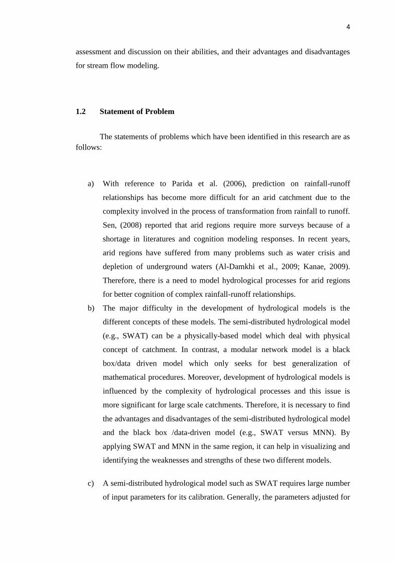
Water scarcity affects the agriculture and food production (Kanae, 2009).

Global warming has been proven to decrease the water availability in arid and semi-

arid regions, where major crop are cultivated. The decreasing water supply for

agriculture and domestic usage will inevitably threaten arid and semi-arid areas. Oki

and Kanae, (2006) has previously showed their geographical distribution of the ratio

between water withdrawal and water availability, and this is as presented in Figure

1.1 (the red coloring indicates a high ratio of water scarcity). Alizadeh, (2007) stated

that in the coming years, Iran will be a water-stressed country.

7

Figure 1.1 Global distribution of water scarcity (i.e., the ratio between water

withdrawal and water availability at each cell of map) by Oki and Kanae, (2006)

By virtue of Rezaitavabeh et al. (2007), one of the logical solutions for water

resource management and promotion of sustainable catchment is to invest in the

harvest and collection of surface water. To date, watershed models have become a

main tool in addressing a wide spectrum of environment and water resource

problems (Singh and Frevert, 2006). Thompson et al. (2004) cited that modeling is

fast and less expensive for the evaluation of different management strategies, and

thus, can help to avoid undesirable outcomes. Until now, researchers are still

persisting on testing and evaluating the stream flow modeling via new techniques to

improve the models’ efficiency and to explore the pros and cons of these

hydrological models.

In terms of hydrology, researchers are now trying to find the advantages and

disadvantages of hydrological modeling to optimize the prediction of rainfall-runoff

relationships. This is to find out the capability of the models for future studies

(Norani et al, 2008). This function gets more important when different types of

8

hydrological models with various concepts have been established. Therefore, it is

essential to identify their strengths and weaknesses. With reference to Boughton

(1984), due to the sparseness of hydrological data in arid and semi-arid areas, the

values vary in the results of every hydrological investigation done in these regions.

Iran suffers from shortage of water because of the arid and semi-arid climatic

conditions, and the country only has an average annual rainfall of 250 mm, which is

only around one-third of the world’s average rainfall. Nevertheless, this region has

the potential to be developed for agricultural purposes and for collecting surface

water. Therefore, the development of hydrological models with different concept

such as SWAT and MNN can assist in the daily flow prediction for the Roodan

region.

In conclusion, this research is significant for the development of the most

popular models (SWAT and MNN) using different types of data in arid region. This

research focuses on the prediction of daily runoff. The development of SWAT and

MNN can assist in the daily stream flow prediction for the Roodan watershed. Also,

daily flow prediction is important for optimal management of the availability of

water resources in every basin. A comparison between SWAT and MNN can be an

opportunity for the evaluation of optimum solutions by modeling the stream flow for

future planning and investment efforts. Finally, this project can show the behavior of

SWAT and MNN models, as a subsidiary tool for hydrologists, in predicting daily

stream flow in large arid region. Last but not least, such study in arid regions can be

interesting and valuable since it has substantially different features in comparison

with other climates, as reported by Sen, (2008).

1.4 Study Objectives

The aim of this study is to make a comparison on the daily stream flow

prediction between the semi-distributed hydrological model, i.e., the soil and water

assessment tool (SWAT), and the black-box/data driven model, i.e., modular neural

network (MNN). The objectives of this study are as follows:

9

1. To model the daily rainfall-runoff relationship of a large arid watershed;

2. To calibrate the SWAT based on the sequential uncertainty fitting-2

algorithm;

3. To propose a MMN using cross-validation technique for modeling the

rainfall-runoff relationship; and

4. To evaluate the performance of SWAT and MNN in large arid climate.

1.5 Scope of the Study

The present study was undertaken to compare the daily stream flow through

two kinds of hydrological models - SWAT and MNN. The scope of this research can

be divided into three parts. The first part involves the development of SWAT model

for daily stream flow simulation. The required data for SWAT are the digital

elevation modeling map (DEM), the hydro-meteorological data (take from year 1988

to 2008), and the soil and land cover maps collected by individual features

availability. A sensitivity analysis and a calibration and uncertainty procedure have

been employed together with the application of the Latin hypercube sampling by one

at a time design (LH-OAT). These are embedded in SWAT version 2009 and the

SUFI-2 algorithm can be found in the SWAT-CUP program (version 2009),

respectively. Finally, the weaknesses and strengths of the SWAT model are observed

and interpreted for the prediction of daily runoff in the large yet arid Roodan

watershed in the southern part of Iran.

The second part of this research involves the development of MNN with two

modules (neural expert) for rainfall-runoff relationships in Roodan watershed using

the hydro-meteorological data from year 1988 to 2008. Such development requires

the training with cross validation and test. Basically, a heuristic method has been

involved to find the optimum architecture and attributed components such as number

of cells, hidden layers, input variables, and coefficients related to the step size and

momentum terms. This study includes the evaluation of uncertainty in the MMN

using the predictive uncertainty (PU) index.

The third part of this research involves the respective evaluations and

comparisons between the daily flow models for the arid and large scale catchment

10

area through general graphical and non-graphical analyses. This comparison has

offered the general features of robustness, accuracy, efficiency, and reliability. This

has made it possible to identify and discuss the advantages and disadvantages of

SWAT versus MNN for daily flow prediction.

1.6 Structure of the Thesis

This thesis consists of five chapters. The first chapter presents the

background, introduction, objectives, and the scope of this research. In the

subsequent chapter, a review of relevant literature and theoretical definitions will be

illustrated using the hydrological cycle. A discussion will also be put forth in regard

to some water resource problems and crisis in arid regions, followed by an

explanation on the runoff concept. Chapter 2 shall also introduce SWAT and MNN

and other attributes of previous publications.

Chapter 3 shall introduce the Roodan watershed together with the analysis of

usual data and the development of SWAT and MNN. Next, Chapter 4 shall explain

the results obtained from the SWAT and MNN models before comparisons are made

for the daily flow predicted by both models. These results were obtained from the

sensitivity analysis, calibration and validation procedures, and the uncertainty

analysis. Lastly, Chapter 5 shall conclude the present study and further suggests

appropriate recommendations for future studies.

256

REFERENCES

Abbaspour, K. C., Van Genuchten, M.Th., Schulin,R., and Schlappi.,E. (1997). A

sequential uncertainty domain inverse procedure for estimating subsurface

flow and transport parameters. Water Resource Research. 33(8), 1879-1892.

Abbaspour, K.C., Johnson, A., and Van Genuchten, M.Th. (2004). Estimating

uncertain flow and transport parameters using a sequential uncertainty fitting

procedure. Vadose Zone Journal. 3(4), 1340-1352.

Abbaspour, K.C., Yang, J., Maximov, I., Siber,R., Bogner,K., Mieleitner,J.,

Zobrist,J., and Srinivasan, R. (2007). Modeling hydrology and water quality

in the pre-alpine/alpineThur watershed using SWAT. Journal of Hydrology.

333, 413-430.

Abbaspour, K.C. (2008). User manual for SWAT-CUP2, SWAT Calibration and

Uncertainty analysis Programs. Swiss Federal Institute of Aquatic Science

and Technology, Duebendorf, Switzerland.

Abbaspour,K.C., Faramarzi, M., Seyed Ghasemi,S., and Yang, H. (2009). Assessing

the impact of climate change on water resources in Iran. Water Resources

Research. 45,1-6.

Ab Rah Saz Shargh. (2009). Comprehensive studies of water resource management

for Roodan watershed, Synthesis report of Roodan. Consulting Water

Resource Engineering Corporation, register code 14800. Mashhad, Iran.

[Accessible web site: www.Abrahsaz.com]

Agarwal, A., Mishra, S.K., Ran, S., and Singh, J.K. (2006). Simulation of runoff and

sediment yield using artificial neural networks. Biosyst. Eng. 94, 597.

Akhavan,S., Abedi-Koupaia, J., Mousavia, S.F., Afyuni, M., Eslaminia, S.S., and

Abbaspour, K.C. (2010). Application of SWAT model to investigate nitrate

leaching in Hamadan-Bahar Watershed, Iran. Agriculture, Ecosystems and

Environment .139, 675-688.

Alibuyog, N.R., Ella, V.B., Reyes, M.R., Srinivasan,R., Heatwole, C., and Dillaha,T.

(2009). Predicting the effects of land use change on runoff and sediment yield

in Manupali river sub-watershed using the SWAT model. International

Agricultural Engineering Journal.18, 15-25.

http://www.abrahsaz.com/

257

Alizadeh, A. (2007). Principles Applied Hydrology. Iran: Emam Reza University.

Al-Damkhi, A.M., Abdul-Wahab, S.A., and AL-Nafisi, A.S. (2009). On the need to

reconsidering water management in Kuwait. Clean Technologies and

Environmental Policy.11, 379-384.

Allen, R.G., Jensen, M.E., Wright, J.L., and Burman, R.D. (1989). Operational

estimates of evapotranspiration. Agron. J. 81,650-662.

Almasri, M.N., and Kaluarachchi, J.J. (2005). Modular neural networks to predict

the nitrate distribution in ground water using the on-ground nitrogen loading

and recharge data. Environmental Modeling & Software. 20,851-871.

Al-Qurashi, A.A.H., Mclntyre, N., Wheater, H., and Unkrich, C. (2008).

Application of the Kineros2 rainfall-runoff model to an arid catchment in

Oman. Journal of Hydrology. 355, 91-105.

Arabi, M., R.S. Govindaraju, M.M. Hantush, and B.A. Engel.(2006). Role of

watershed subdivision on modeling the effectiveness of best management

practices with SWAT. Journal of the American Water Resources Association.

42(2), 513-528.

Arnold, J. G., Allen, P.M., and Bernhardt, G. (1993). A comprehensive surface-

ground water flow model. Journal of Hydrology. 142, 47-69.

Arnold, J.G., Muttiah, R.S., Srinivasan, R., and Allen, P.M. (2000). Regional

estimation of base flow and groundwater recharge in the upper Mississippi

river basin. Journal of Hydrology.227,21-40.

Anctil, F., Perrin, C., and Andreassian, V. (2004). Impact of the length of observed

records on the performance of ANN and of conceptual parsimonious rainfall-

runoff forecasting models. Environmental Modeling and Software. 19, 357-

368.

Anderson, D, and Mcneill,G. (1992). Artificial neural networks technology. Rom

laboratory RL/C3C. Griffiss AFB,NY 13441-5700.

Antar, M.A., Elassiouti,I., and Allam, M.N.(2006). Rainfall-runoff modeling using

artificial neural networks technique: A blue Nile catchment case study.

Hydrological Processes. 20, 1201-1216.

Assad, Y.S.(1997). Application of a neural network technique to rainfall-runoff

modeling. Journal of Hydrology.199,272-294.

ASCE. (2000a). Artificial Neural Networks in Hydrology, part one: Preliminary

Concepts. Journal of Hydrology Engineering, 2, 115-123.

258

ASCE. (2000b). Artificial neural networks in hydrology, part two: Hydrology

applications. Journal of Hydrology Engineering, 2, 124-137.

Babai. (2008). Water in Iran and world, Retrieved November, 11, 2008,

From http://www.mahab.ir/showthread.php?tid=197.

Bahat, Y., Grodek, T., Lekach, J., and Morin, E. (2009). Rainfall-runoff modeling in

a small hyper-arid Catchment. Journal of Hydrology.373, 204-217.

Balon, M., Dehnad, F.(2006). Water crisis in arid and semi-arid regions-an

international challenge. Symposium in Tehran, Iran.12-13, September, 2006.

Bastidas,L.A., Gupta,H.V.,Sorooshian,S.,Shuttleworth,W.J., and Yang,Z.L.(1999).

Sensitivity analysis of land surface scheme using multi criteria methods. In

Wagener,T.,Wheater ,H.S., and Gupta, H.V. Rainfall-runoff modeling in

gauged and un-gauged catchments (pp.26-28). London: Imperial College

press.

Beale, M.H., Hagan,M.T., and Demuth, H.B.(2010).Neural network toolbox 7, users

guide. The math works,Inc.

Bhadra, A., Bandyopadhyay ,A., Singh, R., and Raghuwanshi, N. S.(2010). Rainfall-

runoff modeling: Comparison of two approaches with different data

requirements. Water Resource Manage.24,37-62.

Bian, L., Sun, H., Blodgett, C., Egbert, S., Li W.P., Ran, L.M., and Koussis, A.

(1996). An integrated interface system to couple the SWAT model and

arc/info. Third international conference on integrating GIS and

environmental modeling. Santa Fe: New Mexico.

Bowden, G., Dandy, G.C., and Maier, H.R.(2005). Input determination for neural

network models in water resources applications. Part 1- Background and

methodology. Journal of Hydrology. 301,75-92.

Brooks, K.N., Ffolliott, P.F., Gregersen, H.M., and Thames, J.L. (1991). Hydrology

and the management of watersheds. Ames, IA: Iowa State University Press.

Castellano-Meńdez, M., Gonza´lez-Manteiga,W., Febrero-Bande, M., Prada-

Sańchez, J., and Lozano-Calderoń, R. (2004). Modeling of the monthly and

daily behavior of the runoff of the Xallas river using Box-Jenkins and neural

networks methods. Journal of Hydrology. 296 , 38-58.

Chen. C., and Ding,Y.(2009).The application of artificial neural networks to simulate

melt water runoff of Keqikaer Glacier, south slope of Mt. Tuomuer, western

China, Environmental Geology.57(8),1839-1845.

http://www.mahab.ir/showthread.php?tid=197

259

Chaplot, V. 2005. Impact of DEM mesh size and soil map scale on SWAT runoff,

sediment, and NO3-N loads predictions. Journal of Hydrology. 312(1-4),

207-222.

Chow, V.T., Maidment, D.R., and Mays. L.W. (1988). Applied Hydrology. New

York: McGraw-Hill.

Cigizoglu, H. K., and Alp, M. (2004). Rainfall-runoff modeling using three neural

network methods. Artificial intelligence and soft computing-ICAISC 2004,

lecture notes in artificial intelligence. 3070, 166-171.

Clark, R.T.(1973). Mathematical models in hydrology. In

Wagener,T.,Wheater ,H.S.,Gupta,H.V. Rainfall-runoff modeling in gauged

and un-gauged catchments (pp.26-28). Imperial College press, London.

Clarke, R. (1993). Water: The International Crisis. Cambridge, MA: MIT Press.

Giustolisi, O. and Laucelli, D.(2005) .Improving generalization of artificial neural

networks in rainfall runoff modeling .Hydrological Sciences Journal. 50 (3),

439- 457.

Davie,Tim. (2002). Hydrology as a science. fundamentals of hydrology. London and

New York: Routlege.

Dawson, C.W., and Wilby, R.L.(1998). An artificial neural network approach to

rainfall-runoff modeling, Hydrological Science Journal .43(1), 47-66.

Dawson, C.W., and Wilby, R.L., (2001). Hydrological modeling using artificial

neural networks. Progress in Physical Geography. 25 (1), 80-108.

Demirel, M C., Venancio, A., and Kahya, E. (2009). Flow forecast by SWAT model

and ANN in pracana basin, Portugal. Advanced in Engineering Software, 40,

467-473.

Dingman, S.L. (2002). Physical hydrology. (2nd

ed). Upper Saddle River, N.J.:

Prentice Hall.

Duan, Q., Sorooshian, S., Gupta, H. V., Rousseau, A. N, and Turcotte, R.(2003).

Advances in calibration of watershed models. AGU, Washington, DC.

Ebrahimian, M., Lai Food See., Mohd Hasmadi Ismail., and Ismail Abdul Malek.

(2009). Application of natural resources conservation service-curve number

method for rainfall-runoff estimation with GIS in the Kardeh watershed, Iran.

European Journal of Scientific Research. 34, 575-590.

260

Fayez A. Abdulla., Jumah A. Amayreh., and Adel H. Hossain. (2002). Single event

watershed model for simulating runoff hydrograph in desert regions. Water

Resources Management.16, 221-238.

Faramarzi,M., Abbaspour,K.C., Schulin,R., and Hong,Y. (2009). Modeling blue and

green water resources availability in Iran. Hydrological Processes.23, 486-

501.

Food and Agriculture Organization. 1995. The digital soil map of the world and

derived soil properties. CD-ROM, Version 3.5, Rome.

Freeze, R. A., and Cherry, J. A. (1979). Ground Water. Prentice Hall, Eaglewood

Cliffs N. J.

Flood, I., and Kartam, N. (1994). Neural networks in civil engineering, I: Principles

and understanding. Journal of Computing in Civil Engineering. 8(2), 131-148.

Foltz, R. C. (2002). Iran’s water crisis: cultural, political, and ethical dimensions.

Journal of Agricultural and Environmental Ethics.15, 357-380.

Francos, A., Elorza, F.J., Bouraoui, F., Galbiati, L. and Bidoglio, G. (2001).

Sensitivity analysis of distributed environmental simulation models:

understanding the model behavior in hydrological studies at the catchment

scale. Reliability Engineering and System Safety. 79, 205-218.

Frot, E., and Wesemael, B. (2009). Predicting runoff from semi-arid Hill slopes as

source areas for water harvesting in the Sierra de Gador, southeast Spain.

Catena. 79, 83-92.

Gassman, P. W., Reyes, M. R., Green, C. H. and Arnold, J. G. (2007). The Soil and

Water Assessment Tool: historical development, applications and future

research directions. Trans. Am. Soc. Agric. Biol. Engrs .50(4), 1211-1250.

Ghahreman, B. and Hatamiyazdi, A. (2007). Reviewing and generalizing rainfall-

runoff relationships for un-gauged watersheds case study: Nahreyn and Kerit

in Tabas, Yazd province. Secondary Conference of Water Resource

Management. IRAN. Available at: http://www.civilica.com/Paper-WRM02-

WRM02_033.html.

Ghaffari, G., Keesstra, S.,Ghodousi, J., and Ahmadi ,H .(2010). SWAT-simulated

hydrological impact of land-use change in the Zanjanrood basin, northwest

Iran. Hydrological Processes. 24, 892-903.

http://www.civilica.com/Paper-WRM02-WRM02_033.html

http://www.civilica.com/Paper-WRM02-WRM02_033.html

261

Ghumman, A.R., Ghazaw.,Y.M., Sohail,A.R., and Watanabe,K. (2011).Runoff

forecasting by artificial neural network and conventional model. Alexandria

Engineering Journal.50,345-350.

Gosain,A.K., Mani,A. and Dwivedi,C. (2009). Hydrological modelling review.

Climawater. Report NO.1.

Green,C.H., and Griensven, A.V.(2008). Auto calibration in hydrologic modelling:

using SWAT2005 in small-scale watersheds. Environmental Modelling and

Software .23,422-434.

Gupta, H.V.,Sorooshian,S., and Yapo,P.O. (1998). Toward improved calibration of

hydrologic models: multiple and non commensurable measures of

information. In Wagener,T., Wheater ,H.S., and Gupta,H.V. Rainfall-runoff

modeling in gauged and un gauged catchments. (pp.41-45) Imperial College

press, London.

Hantush, M.M., and Kalin, L. (2005). Uncertainty and sensitivity analysis of runoff

and sediment yield in a small agricultural watershed with kineros2.

Hydrological Sciences Journal. 50(6),1151-1172.

Hargreaves, G.L., Hargreaves, G.H., and Riley, J.P.(1985). Agricultural benefits for

Senegal River Basin. J. Irrig. and Drain. Engr. 111(2),113-124.

Hernandez, M., Miller, S.N., and Goodrich, D.C.(2000). Modeling runoff response to

land cover and rainfall spatial variability in semi-arid watersheds.

Environmental Monitoring Assessment. 64, 285-298.

Hu,T.S., Lam,K.C., and Ng, S.T. (2001). River flow time series prediction with a

range-dependent neural network, Hydrology Science Journal. 46(5), 729-745.

Hjelmfelt, A.T., 1980. Empirical-investigation of curve number technique. Journal of

the Hydraulics and Engineering Division-ASCE.106 (9), 1471-1476.

Huang,Z., Xue,B., and Pang,Y. (2009). Simulation on stream flow and nutrient

loading in Gucheng Lake, Low Yangtze river basin, based on SWAT model.

Quaternary International.208,109-115.

Heuvelmans, G., Muys,B., and Feyen, J.(2004). Analysis of the spatial variation in

the parameters of the SWAT model with application in Flanders, Northern

Belgium. Hydrology and Earth System Sciences. 8(5),931-939.

262

International Water Management Institute. (2006). Balancing Water for Food and

Other Ecosystem Services. Retrieved December, 20, 2009, From

http://www.lk.iwmi.org/WWF4/html/action_4.htm .

Imrie, C.E., Durucan, S., and Korre, A. (2000). River flow prediction using artificial

neural networks: Generalization beyond the calibration range. Journal of

Hydrology. 233 (1-4), 138-153.

Jain, A.K., Mao, J., and Mohiuddin, K.M. (1996). Artificial neural networks a

tutorial. March. IEEE, 31-44.

Jajarmizadeh, M., Sobri Harun., Salarpour, M. (2012a). A review on theoretical

consideration and types of models in hydrology. Journal of Environmental

Science and Technology. 5(5),249-261.

Jajarmizadeh,M., SobriHarun., RoziAbdullah., and Salarpour,M.(2012b).Using Soil

and Water Assessment Tool for flow simulation and assessment of sensitive

parameters applying SUFI-2 algorithm. Caspian Journal of Applied Sciences

Research. 2(1): 37-47.

Jayakrishnan,R., Srinivasan,R., Santhi,C., and Arnold, J.G.(2005). Advances in the

application of the SWAT model for water resource management.

Hydrological Processes. 19, 749-762.

Jha, M. (2009). Hydrologic simulation of the Maquoketa river watershed using

SWAT. Center for agricultural and rural development Iowa state university.

Working paper 09-WP 492.

Junfeng, C., Xiubin,L., and Ming, Z. (2005). Simulating the impacts of climate

variation and land-cover changes on basin hydrology; A case study of the

Suomo basin. Science in China Ser. D Earth science. 48(9),1501-1509.

Kalteh, A.M., Hjorth, P., and Berndtsson, R. (2008). Review of the self-organizing

map (SOM) approach in water resources: Analysis, modeling and application.

Environmental Modeling and Software.23,835-845.

Kanae, S. (2009). Global Warming and the Water Crisis. Journal of Health

Science.55, 860-864.

Kannan,N., White.S.M., Worrall.,F., and Whelan. M.J.(2007). Sensitivity analysis

identification of the best evapotranspiration and runoff options for

hydrological modeling in SWAT 2000. Journal of Hydrology. 332,456-466.

Karamouz,M., and Araghinejad,S. (2003). Engineering Hydrology. Iran: Amir Kabir

University publication.

http://www.lk.iwmi.org/WWF4/html/action_4.htm

263

Kim, G. S., Borros, A. P. (2001). Quantitative flood forecasting using multi sensor

data and neural networks. Journal of Hydrology.246, 45-62.

Kisi, O., Moghaddam Nia, A., Ghafari Gosheh, M ., Jamalizadeh Tajabadi., M.R.,

and Ahmadi, A.(2012). Intermittent stream flow forecasting by using several

data driven techniques. Water Recourse Management. 26,457-474.

Kisi, O. (2008). River flow forecasting and estimation using different artificial neural

network techniques. Hydrology Research. 39(1), 27-40.

Kneale, P., See, L., and Smith, A. (2001). Towards defining evaluation measures for

neural network forecasting models. Proceedings of the 6th

international

conference on geocomputation. University of Queensland, Brisbane,

Australia. GeoComputation, Leeds, United Kingdom.

Konukcue, F., Istanbulluoglu, A., and Kocaman,I. (2005). Determination of the

water yields for small basins in semi-arid area: application of the modified

Turk method to the Turkey’s condition. Journal Central European

Agriculture. 6, 263-268.

Krause,P., Boyle., D.P., and Base, F. (2005). Comparison of different efficient

criteria for hydrological model assessment. Advanced Geosciences.5,89-97.

Krysanova, V., and Arnold, J.G. (2009). Advances in ecohydrological modeling with

SWAT-A review. Hydrological Science Journal. 53(5), 939-947.

Kuok, K.K. (2010). Parameter optimization methods for calibrating tank model and

neural network model for rainfall runoff modeling. PhD dissertation.

University Teknologi Malaysia, Skudai.

Legates. D .R., and McCabe, G. J. (1999). Evaluating the use of ‘‘Goodness of Fit’’

measures in hydrologic and hydro-climatic model validation. Water

Resources Research. 35(1), 233-241.

Lenhart, T., Eckhardt, K., Fohrer, N., and Frede, H.G. (2002). Comparison of two

different approaches of sensitivity analysis. Physics and Chemistry of the

Earth. 27, 645–654.

Leon, L.F., Soulis, N.K., and Farquhar,G.J. (2002). Modelling diffuse pollution with

a distributed approach. Journal Water Science and Technology. 45(9),149-

156.

Lewarne., M.(2009). Setting up ARCSWAT hydrological model for the Verlorenvlei

catchment. Master dissertation. Stellenbosch University.

264

Maier, H.R., and Dandy, G.C. (2000). Neural networks for the prediction and

forecasting of water resources variables: A review of modeling issues and

applications. Environment Model Software.15,101-124.

Malekian, A., Saravi. M.M., and Mahdavi, M. (2004). Modified soil antecedent

moisture for curve number method. EUROSOL Conference. Sep 4- 12,

Freiburg Germany.

McIntyre, N., Al-Qurashi, A., and Wheater, H. (2009). Regression analysis of

rainfall-runoff data from an arid catchment in Oman. Hydrological Science

Journal. 52, 1103-1118.

Melching, C.S.,Yen, B.C., and Wenzel, H.G., Jr. (1990). A reliability estimation in

modeling watershed runoff with uncertainties. In Wagener,T.,Wheater ,H.S.,

and Gupta,H.V. Rainfall-runoff modeling in gauged and ungauged

catchments( pp.4-7). London Imperial College press.

Melching, C.S.(1995). Reliability estimation. In Wagener,T., Wheater, H.S., Gupta,

H.V. Rainfall-runoff modeling in gauged and un-gauged catchments (pp.41-

45). London: Imperial College presss.

Menhaj, M.B. (2010). Computational intelligence, fundamentals of neural networks.

Iran: Amir Kabir university publication.

Minns, A.W., and Hall,M.J. (1996). Artificial neural networks as rainfall-runoff

models, Hydrological Sciences Journal. 41 (3), 399-418.

Mishra, S.K., Singh, V. p., Sansalone, J.J., and Aravamuthan, V. (2003). A Modified

SCS-CN Method: Characterization and Testing. Water Resources

Management. 17,37-68.

Misra, D., Oommen, T., Agarwal, A., Mishra,S. K., and Thompson, A. M.(2009).

Application and analysis of support vector machine based simulation for

runoff and sediment yield. Biosystems Engineering. 3, 527-535.

Moriasi, D.N., Arnold, J.G., Van Liew, M.W., Binger, R.L., Harmel, R.D., and Veith,

T. (2007). Model evaluation guidelines for systematic quantification of

accuracy in watershed simulations. Trans.ASABE .50(3), 885-900.

Morid, S., Ghaemi. H., Mir Abolghasemi, H., and Abediny M. (2001). Evaluation of

the HEC-1 Model for Flood Forecasting and Solution in the Hormozgan

Province, Iran. Journal of Environment Hydrology. 9,1-8.

265

Morid, S., Gosain A.K., Keshari, A.K.(2002). Comparison of the SWAT model and

ANN for daily simulation of runoff in snowbound un-gauged catchments.

Fifth international conference on hydroinformatics, Cardiff, UK.

Mou, L., Fuqiang. T., and Heping. H. (2009). Artificial neural network model of

runoff prediction in high and mountainous regions: A case study in the source

drainage area Urumqi River. Journal of Hydroelectric Engineering. 28(1)62-

67.

Mutlu, E., Chaubey, I., Hexmoor, H., and Bajwa,S. G.(2008). Comparison of

artificial neural network models for hydrologic predictions at multiple

gauging stations in an agricultural watershed, Hydrological Processes. 22,

5097-5106.

Mwakalila, S., Campling, P., Feyen, J., Wyseure, G., and Beven, K. (2001).

Application of a data-based mechanistic modeling (DBM) approach for

predicting runoff generation in semi-arid regions. Hydrological Processes. 15,

2281-2295.

Nayebi, M., Khalili, D., Amin, S., and Zand-Parsa, S.H. (2006). Daily stream flow

prediction capability of artificial neural networks as influenced by minimum

air temperature data. Biosystems Engineering. 95 (4), 557-567.

Negnevitsky,M. (2005). Artificial intelligence. (2nd

ed). England: Pearson Education

Limited.

Neitsch S.L, Arnold J.G, Kiniry J.R, and William J.R. (2005). Soil and water

assessment tool theoretical documentation (version 2005). Grassland, soil

and water research laboratory, agricultural research service, and blackland

research center, texas agricultural experiment station: Temple, Texas 76502,

USA, 494.

Neitsch, S.L., Arnold, J.G., Kiniry, J.R., Srinvasan, R., and Williams, J.R. (2010).

Soil and water assessment tool, input/output file documentation, version2009.

Soil and water research laboratory, agricultural research service, and

blackland research center, texas Agrilife research. Texas water resources

institute technical report No.365: Texas A&M University, USA.

Nie, W., Yuan, Y., Kepner, W., Nash, M.S., Jackson, M., and Erickson, C. (2011).

Assessing impact of land use and land cover changes on hydrology for the

upper San Pedro watershed. Journal of Hydrology. 407, 105-114.

266

Nourani,N., and Kalantari, M. (2010). Integrated Artificial Neural Network for

Spatiotemporal Modelling of Rainfall-Runoff-Sediment Processes.

Environmental Engineering Science. 27(5), 411-422.

Irawan,N. (2005). Rainfall-runoff modeling using artificial neural network method.

Ph.D dissertation. University Technology Malaysia. Skudai.

Oki, T. and Kanae, S. (2006). Global hydrological cycles and world water resources.

Science. 313,1068-1072.

Openshaw, S., and Openshaw, C.(1997). Artificial intelligence in geography.

England: John Wiley and Sons.

Oeurng , C., Sauvage, S., and Sanchez-Perez, J. (2011). Assessment of hydrology,

sediment and particulate organic carbon yield in large agricultural catchment

using SWAT model. Journal of Hydrology. 401,145-153.

Pai, N., and Saraswat, D. (2011). SWAT 2009-LUC:A tool to activate the land use

change module in SWAT 2009. American Society of Agricultural and

Biological Engineers. 54(5):1649-1658.

Parasuraman, K., Elshorbagy, A., and Carey, S.K. (2006). Spiking modular neural

networks: A neural network modeling approach for hydrological processes.

Water resources research. 42,1-14.

Parida, B.P., Moalafhi, D.B., and Kenabatho, P.K. (2006). Forecasting runoff

coefficient using ANN for water resources management: The case of

Notwane catchment in Eastern Botswana. Physics and Chemistry of the

Earth. 31, 928-934.

Patil, J.P., Sarangi. A., Singh, A.K., and Ahmad, T. (2008). Evaluation of modified

CN methods for watershed runoff estimation using a GIS-based interface.

Biosystems Engineering. 100,17-146.

Pallat, J.(2004). SPSS survival manual. Amazon publisher Inc.

Patra, K.C. (2008) .Hydrology and water resources engineering. U.K.: Alpha

Science International Ltd.

Parajuli, P.B., Nelson, N.O., Frees, L.D., and Mankin, K.R. (2009). Comparison of

AnnAGNPS and SWAT model simulation results in USDA-CEAP

agricultural watersheds in south-central Kansas. Hydrological Processes.

23,784-763.

267

Pidwirny , M.(2006). Global Distribution of Precipitation. Fundamentals of Physical

Geography, 2nd

Edition. Retrieved December, 22, 2009 from

http://www.physicalgeography.net/fundamentals/8g.html.

Priestley, C.H.B., and Taylor, R.J. (1972). On the assessment of surface heat flux and

evaporation using large-scale parameters. Mon. Weather. Rev.100:81-92.

Raneesh, S.G., Thampi. K.Y., and Surya, T.V. (2010). Influence of scale on SWAT

model calibration for stream flow in a river basin in the humid tropics. Water

Resource Manage. 224,4567-4578.

Rezaitavabeh, K., Taheriazad, L., Mahmodi,M., and Yazdanpanah ,A. (2007).

Reviewing of limitations in water resource management in Iran and finding

the solutions for sustainable developing. The ninth national irrigation

seminar. Available at:http://www.civilica.com/Paper-ABYARI09-

ABYARI09_079.html.

Rezaeian Zadeh, M ., Seifollah, A., Khalili, D., and Singh, V.P. (2010). Daily

outflow prediction by multi layer perceptron with logistic sigmoid and

tangent sigmoid activation functions. Water Resources Management. 24 (11),

2673-2688.

Riad, S.,Mania. L.,Bouchaou. L., and Najjar.Y. (2004a). Predicting catchment flow

in a semi arid region via an artificial neural network technique. Hydrological

Processes.18,2387-2393.

Riad, S. Mania, J., Bouchaou, L., and Najjar,Y. (2004b). Rainfall-runoff model using

an artificial neural network approach. Mathematical and Computer Modeling.

40, 839-846.

Rodier, J. A. (1985). Aspects of arid zone hydrology. In Rodda J.C.(Ed). Facets of

Hydrology, vol. II. (205-247). Chichester, UK: John Wiley & Sons Ltd.

Rogers, G.O., and DeFee B.B. (2005). Long-term impact of development on a

watershed: Early indicators of future problems. Land Scape and Urban

Planning. 73(2-3), 215-233.

Rostamian, R., Aazam. J, Afyuni, M., Mousavi., F., Heidarpour, M., Jalalian, A, and

Abbaspour, K. C. (2008). Application of a SWAT model for estimating

runoff and sediment in two mountainous basins in central Iran. Hydrological

Sciences Journal, 53(5), 977-988.

Sajikumar, N., and Thandaveswara, B. S. (1999). A non-linear rainfall-runoff model

using an artificial neural network. Journal of Hydrology. 216, 32-5l.

http://www.physicalgeography.net/fundamentals/8g.html

http://www.civilica.com/Paper-ABYARI09-ABYARI09_079.html.

http://www.civilica.com/Paper-ABYARI09-ABYARI09_079.html.

http://www.engineeringvillage.com/controller/servlet/Controller?CID=quickSearchCitationFormat&searchWord1=%7BRostamian%2C+Rokhsare%7D&section1=AU&database=131073&yearselect=yearrange&sort=yr

http://www.engineeringvillage.com/controller/servlet/Controller?CID=quickSearchCitationFormat&searchWord1=%7BJaleh%2C+Aazam%7D&section1=AU&database=131073&yearselect=yearrange&sort=yr

http://www.engineeringvillage.com/controller/servlet/Controller?CID=quickSearchCitationFormat&searchWord1=%7BAfyuni%2C+Majid%7D&section1=AU&database=131073&yearselect=yearrange&sort=yr

http://www.engineeringvillage.com/controller/servlet/Controller?CID=quickSearchCitationFormat&searchWord1=%7BMousavi%2C+Seyed+Farhad%7D&section1=AU&database=131073&yearselect=yearrange&sort=yr

http://www.engineeringvillage.com/controller/servlet/Controller?CID=quickSearchCitationFormat&searchWord1=%7BHeidarpour%2C+Manouchehr%7D&section1=AU&database=131073&yearselect=yearrange&sort=yr

http://www.engineeringvillage.com/controller/servlet/Controller?CID=quickSearchCitationFormat&searchWord1=%7BJalalian%2C+Ahmad%7D&section1=AU&database=131073&yearselect=yearrange&sort=yr

http://www.engineeringvillage.com/controller/servlet/Controller?CID=quickSearchCitationFormat&searchWord1=%7BAbbaspour%2C+Karim+C.%7D&section1=AU&database=131073&yearselect=yearrange&sort=yr

268

Schuol, J., Abbaspour, K.C., Srinivasan, R., and Yang ,H. (2008). Estimation of

freshwater availability in the West African sub-continent using the SWAT

hydrologic model. Journal of Hydrology.352,30-49.

Sen, Z. (2008). Hydrograph and unit hydrograph derivation in arid regions.

Hydrological Processes.21, 1006-1014.

Senthil Kumar, A. R., Sudheer ,K. P., Jain, S. K., and Agarwal, P. K. (2005).

Rainfall-runoff modelling using artificial neural networks: Comparison of

network types. Hydrological Processes.19,1277-1291.

Setegn, S.G., Srinivasan, R., Melesse, A.M., and Dargahi, B. (2010). SWAT model

application and prediction uncertainty analysis in the Lake Tana basin,

Ethiopia. Hydrological Processes. 24,357-367.

Shaw, E.M. (1994). Hydrology in Practice. London: Chapman and Hall.

Shakir, A., and Sharda, V.N. (2008). A comparison of curve number based methods

for runoff estimation from Small Watersheds in semi-arid region of India.

Hydrology Research. 39, 191-200.

Shamseldin, A. Y. (1997). Application of neural network technique to rainfall-runoff

modeling .Journal of Hyrology.199, 272-294.

Singh,V.P. (1995). Computer models of watershed hydrology. Highlands Ranch, CO:

Water Resources Publications.

Singh, V.P., and Frevert, D.K. (2006). Watershed models. U.S:Taylor & Francis

Group.

Singh, A., Imtiyaz, M., Isaac, R.K., and Denis, D.M. (2012).Comparison of soil and

water assessment tool (SWAT) and multilayer perceptron (MLP) artificial

neural network for predicting sediment yield in the Nagwa agricultural

watershed in Jharkhand, India. Agricultural Water Management. 104,113-120.

Sivakumar, B., Jayawardena, A.W., and Fernando, T.M.K.G. (2002). River flow

forecasting: use of phase-space reconstruction and artificial neural networks

approaches, Journal of Hydrology. 265 (1-4 ), 225-245.

Smith, J., and Eli, R.N. (1995). Neural-network models of rainfall-runoff process,

Journal of Water Resources Planning and Management. 121(6), 499-508.

Srinivasulu, S., and Jain, A.(2006). A comparative analysis of training methods for

artificial neural network rainfall-runoff models. Applied Soft Computing. 6,

295-306.

269

Srivastava, P., McNair, J.N., and Johnson, T.E.(2006). Comparison of process-based

and artificial neural network approaches for stream flow modeling in an

agricultural watershed. Journal of the American Water Resources Association.

42(3), 545-563.

Soil Conservation Service. (1972). Section 4: Hydrology in national engineering

handbook. SCS.

Sorman, A.U., and Abdulrazzaq, J.(1993). Infiltration-recharge through Wadi beds

in arid region. Hydrological Sciences Journal. 38 (3), 173-186.

Soulis, K.X., Valiantzas, J.D., Dercas, N., and Londra., P.A. (2009). Analysis of the

runoff generation mechanism for the investigation for the SCS-CN method

applicability to a partial area experimental watershed. Hydrology and Earth

System Sciences Discussions. 6, 373-400.

Talebizadeh, M., Morid,S., Ayyobzadeh, S.A., and Ghasemzadeh, M.(2010).

Uncertainty analysis in sediment load modeling using ANN and SWAT

models. Water Resource Manage. 24, 1747-1761.

Thompson, J.R., Sorenson, H.R., Gavin, H., and Refsgard, A. (2004). Application of

the coupled MIKE SHE/MIKE 11 modeling system to a lowland wet

grassland in southeast England. Journal of Hydrology. 293(2), 151-179.

Tokar, A. S., and Johnson, P. A. (1999). Rainfall-runoff modeling using artificial

neural networks. Journal of Hydrology Engineering. 4(3), 232-239.

Toth, E., and Brath, A., (2007). Multistep ahead stream flow forecasting: role of

calibration data in conceptual and neural network modeling. Water Resources

Research. 43(11), W11405.

Tombul, M., and Ogul, E. (2006). Modeling of rainfall-runoff relationship at semi-

arid small catchments using artificial neural networks. Lecture notes in

control and information sciences (LNCIS), intelligent control and automation.

344, 309-318.

Tripathi, MP., Panda, R.K., Raghuwanshi, N.S., and Singh, R. (2004). Hydrological

modeling of a small watershed using generated rainfall in the soil and water

assessment tool model. Hydrological Process. 18, 1811-1821.

Vandenberghe, V., Van Griensven, A., and Bauwens, W. (2001). Sensitivity analysis

and calibration of the parameters of ESWAT: Application to the river Dender.

Water Science and Technol.43(7), 295-301.

270

Van Griensven, A., and Meixner, T. (2003). Sensitivity, optimization and uncertainty

analysis for the model parameters of SWAT. 2nd

International SWAT

Conference. Bari, Italy, 1-4 July.

Van Griensven, A., Meixner, T., Grunwald S., and Srinivasan R. (2005). Evaluation

Methods for SWAT Models. 3rd

International SWAT Conference. Zurich,

Switzerland, 11-15 July.

Van Griensven, A., Meixner,T., Grunwald,S., Bishop,T., Diluzio,M., and

Srinivasan,R. (2006). A global sensitivity analysis tool for the parameters of

multi- variable catchment models. Journal of Hydrology. 324, 10-23.

Van Liew, M. W., Arnold, J. G., Garbrecht, J. D. (2003). Hydrologic simulation on

agricultural watersheds: Choosing between two models. Trans. ASAE. 46(6),

1539-1551.

Wgener,T.(1998). Developing a prototype knowledge based system to support

rainfall-runoff modelling. In Wagener, T., Wheater, H.S., and Gupta,H.V.

rainfall-runoff modeling in gauged and un-gauged catchments (pp.4-7).

London Imperial College press.

Wagener, T., Wheater, H.S., and Gupta, H.V. (2004). Rainfall-runoff modelling in

gauged and un-gauged catchments. London: Imperial College Press.

Wang, S., Kang, S., Zhang, Lu., and Li ,F.(2008). Modelling hydrological response

to different land-use and climate change scenarios in the Zamu River basin of

northwest China. Hydrological Process. 22, 2502-2510.

Wang, W., Van Gelder, P.H.A.J.M., Vrijling ,J.K., and Jun Ma. (2006). Forecasting

daily stream flow using hybrid ANN models. Journal of Hyrology.324, 383-

399.

Wales, J. (2009). Water Supply and Sanitation in Iran. Retrieved December, 4, 2009.

From http://en.wikipedia.org/wiki/Water_supply_and_sanitation_in_Iran.

Warren, V.Jr., and Gary, L.L. (2003). Introduction to Hydrology. (5th

ed). Upper

Saddle, River, NJ: Prentice Hall.

Wilby, R.L.(1997). Contemporary hydrology. England: John and Sons.

Winchell. M., Srinivasan, R., Di Luzio, M., and Arnold, J. (2010). Arc SWAT

interface for SWAT 2009. Users’guide. Grassland,soil and water research

laboratory, agricultural research service and blackland research center, Texas

agricultural experiment station: Temple, Texas 76502, USA,495.

http://en.wikipedia.org/wiki/Water_supply_and_sanitation_in_Iran

271

World Meteorological Organistaion. (1975). Inter-comparison of conceptual models

used in operational hydrological forecasting. World meteorological

Organisation, Techinical report No 429, Geneva, Switzerland.

World Water Council. (2009). Water Crisis. Retrived December, 20, 2009, from

http://www.worldwatercouncil.org/index.php?id=25.

Wu, Jy. S., Han, J., Annambhotla, S., and Bryant, S. (2005). Artificial neural

networks for forecasting watershed runoff and stream flows. Journal of

Hydrologic Engineering. 10(3), 216-222.

Wu, C.L., and Chau, K.W. (2011). Rainfall-runoff modeling using artificial neural

network coupled with singular spectrum analysis. Journal of Hydrology.

399,394-409.

Wu, J. (2012). Prediction of rainfall time series using modular RBF neural network

model coupled with SSA and PLS. ACIIDS 2012. Part II, LNAI 7197(pp.

509-518). Springer,Verlag Berlin Heidelberg.

Xu, Z.X., Pang, J.P., Liu, C.M., and Li, J.Y. (2009a). Assessment of runoff and

sediment yield in the Miyun reservoir catchment by using SWAT model.

Hydrological Process. 23, 3619-3630.

Xu, J., Zaho, J., Zhang, W., HU, Z., and Zheng, Z (2009b). Mid-short-term daily

runoff forecasting by ANNs and multiple process-based hydrological models.

IEEE youth conference on information, computing and telecommunication.

20-21 September. China: IEEE computer society. 526-529.

Xu,Qin., Ren, L., Yu, Z., Yang, Bang., and Wang, G.(2008). Rainfall-runoff

modelling at daily scale with artificial neural networks. 4th

international

conference on natural computation, October,18-20 ICNC. 2, 504-508.

Yakhkeshi,E. (2007). Application of artificial neural network models in flood

warning system preparation. Ph.D dissertation. Islamic Azad University,

branch of Tehran.

Yang, J., Reichert, P., Abbaspour, K.C., Xia, J., and Yang, H. (2008). Comparing

uncertainty analysis techniques for a SWAT application to Chaohe Basin in

China. Journal of Hydrology. 358, 1-23.

Yapo, P. O., Gupta, V. H., and Sorooshian, S. (1996). Automatic calibration of

conceptual rainfall-runoff models: Sensitivity to calibration data. Journal of

Hydrology.181, 23-48.

http://www.worldwatercouncil.org/index.php?id=25

272

Ye. X.C., Viney, N.R., and Zhang, Q. (2009). Effects of spatial resolution of soil data

on hydrological processes modeling A case study using the SWAT model.

The proceeding of 18th

world IMACS congress and MODSIM09 international

congress on modeling and simulation. July 13-17, Griffith university, pp

3216-3222.

Zhang, B., and Govindaraju, S. (2000). Prediction of watershed runoff using

Bayesian concepts and modular neural networks. Water Resource Research.

36 (3), 753- 762.

milad jajarmizadeh -...

Documents