ABSTRAK

Katakan G ialah suatu graf. Nombor persilangan bagi graf G, ditandakan

cr(G), adalah bilangan persilangan tepi-tepinya yang minimum daripada lukisan-

lukisan G pada satah. Kepencongan bagi graf G, ditandakan sk(G), adalah

bilangan minimum tepi dalam G yang perlu dihapuskan untuk menghasilkan

satu graf satahan.

Dalam Bab 1 tesis ini, sebahagian sifat asas dan takrif mengenai graf akan

diberikan.

Dalam Bab 2, kami membentangkan sebahagian keputusan-keputusan yang

telah diketahui mengenai nombor persilangan bagi graf dan juga satu kriteria

penyatahan bagi sesuatu graf.

Dalam Bab 3, kami memberikan satu tinjauan mengenai kepencongan bagi

graf dan memperkenalkan sebahagian graf yang bersifat π − skew.

Keputusan utaman dalam tesis ini dibentangkan dalam bab terakhir. Kami

memperolehi beberapa hasil mengenai kepencongan bagi cantuman dua graf.

Kemudian, kami menggunakan keputusan tersebut untuk menentukan secara

lengkapnya bagi kepencongan graf k-bahagian lengkap untuk k = 2, 3, 4.

i

ABSTRACT

Let G be a graph. The crossing number of G, denoted as cr(G), is the minimum

number of crossings of its edges among all drawings of G in the plane. The

skewness of a graph G, denoted as sk(G), is the minimum number of edges in

G whose deletion results in a planar graph.

In Chapter 1 of this thesis, some preliminaries and definitions concerning

graphs are given.

In Chapter 2, we present some known results on crossing numbers of graphs

and also a planarity criterion for a graph.

In Chapter 3, we provide a survey on skewness of graphs and introduce

some graphs which are π − skew.

The main results of this thesis are presented in the last chapter. We prove

some results concerning the skewness for the join of two graphs. We then

use these results to determine completely the skewness of complete k-partite

graphs for k = 2, 3, 4.

ii

ACKNOWLEDGEMENTS

I would like to express my sincere gratitude to my supervisor, Professor

Chia Gek Ling for supervising my research. His guidance, insightful comments

and corrections are invaluable to me throughout my study.

A special thank to Professor Angelina Chin Yan Mui and Madam Budiyah

binti Yeop for their support and advice. Last but not the least, I would like

to thank my family for their unshakable support and faith.

iii

Contents

ABSTRAK . . . . . . . . . . . . . . . . . . . . . . . . . . . . . . . i

ABSTRACT . . . . . . . . . . . . . . . . . . . . . . . . . . . . . . ii

ACKNOWLEDGEMENTS . . . . . . . . . . . . . . . . . . . . . iii

1 Introduction 1

1.1 Introduction . . . . . . . . . . . . . . . . . . . . . . . . . . . . . 1

1.2 Preliminaries and Definitions . . . . . . . . . . . . . . . . . . . . 2

1.3 New Graphs from Old . . . . . . . . . . . . . . . . . . . . . . . 4

2 Crossing Number 7

2.1 Introduction . . . . . . . . . . . . . . . . . . . . . . . . . . . . . 7

2.2 Crossing Number of Some Families of Graphs . . . . . . . . . . 8

2.2.1 Complete Bipartite Graphs . . . . . . . . . . . . . . . . 9

2.2.2 Complete Graphs . . . . . . . . . . . . . . . . . . . . . . 10

iv

2.2.3 Complete Tripartite Graphs . . . . . . . . . . . . . . . . 12

2.2.4 Join of Graphs . . . . . . . . . . . . . . . . . . . . . . . 13

2.2.5 Generalized Petersen Graphs . . . . . . . . . . . . . . . . 16

2.3 Planarity Criterion . . . . . . . . . . . . . . . . . . . . . . . . . 18

2.4 Crossing-critical Graphs . . . . . . . . . . . . . . . . . . . . . . 20

2.4.1 Definitions . . . . . . . . . . . . . . . . . . . . . . . . . . 20

2.4.2 Some Ideas and Examples . . . . . . . . . . . . . . . . . 20

3 Skewness of Graphs 22

3.1 Introduction . . . . . . . . . . . . . . . . . . . . . . . . . . . . . 22

3.2 π − skewness . . . . . . . . . . . . . . . . . . . . . . . . . . . . 23

3.3 Known Results . . . . . . . . . . . . . . . . . . . . . . . . . . . 25

3.4 Skewness-critical Graphs . . . . . . . . . . . . . . . . . . . . . . 27

4 Skewness of the Join of Graphs 28

4.1 Introduction . . . . . . . . . . . . . . . . . . . . . . . . . . . . . 28

4.2 Join of Graphs . . . . . . . . . . . . . . . . . . . . . . . . . . . 29

4.3 Complete Tripartite Graphs . . . . . . . . . . . . . . . . . . . . 31

4.4 Complete 4-partite Graphs and More . . . . . . . . . . . . . . . 34

v

4.5 Conclusion . . . . . . . . . . . . . . . . . . . . . . . . . . . . . . 41

REFERENCES . . . . . . . . . . . . . . . . . . . . . . . . . . . . . 42

vi

List of Figures

1.1 The Petersen graph P (5, 2) . . . . . . . . . . . . . . . . . . . . . 6

2.1 A drawing of K4,5 with 8 crossings . . . . . . . . . . . . . . . . 9

2.2 Complete graphs on 5 and 6 vertices . . . . . . . . . . . . . . . 11

2.3 Complete tripartite graph K1,3,5 with 10 crossings . . . . . . . . 12

2.4 The graph Cm + Cn . . . . . . . . . . . . . . . . . . . . . . . . . 14

2.5 The graph K4 + Pn . . . . . . . . . . . . . . . . . . . . . . . . . 16

2.6 . . . . . . . . . . . . . . . . . . . . . . . . . . . . . . . . . . . . 21

3.1 A planar graph obtained by removing (m−2)(n−2) edges from

Km,n. . . . . . . . . . . . . . . . . . . . . . . . . . . . . . . . . . 26

4.1 Hm,n,r with r faces . . . . . . . . . . . . . . . . . . . . . . . . . 34

vii

Chapter 1

Introduction

1.1 Introduction

In recent years, graph theory has been one of the most rapidly growing areas

of mathematics. Graph theory and its applications can be found not only

in other branches of mathematics such as algebra, geometry, combinatorics

and topology, but also in other scientific disciplines, ranging from computer

sciences, engineering, management sciences and life sciences.

Much effort has gone into finding the crossing number and skewness of

graphs. Building from these researches, this thesis will continue from these

work, particularly of that published in [4]. In this thesis, we determine com-

pletely the skewness of complete k-partite graphs for k = 2, 3, 4.

1

1.2 Preliminaries and Definitions

In this section, the basic definitions which will be frequently referred through-

out this thesis are presented. For those terms and definitions not included

here, the reader is referred to [2], [40] and [41].

A graph G = (V,E) consists of a finite non-empty vertex set V (G) and

a finite (possibly empty) edge set E(G). The elements in V (G) (respectively

E(G)) are called vertices (respectively edges). The number of vertices of G

is the order of G and is denoted as |V (G)|. The number of edges of G is the

size of G and is denoted as |E(G)|.

We say that a graph G is finite if both its vertex set and edge set are finite.

A graph with no vertices (and hence no edges) is the empty graph. In this

thesis, we confine our attention to finite graphs. Any graph with only one

vertex is trivial.

Two vertices u and v of a graph G are adjacent if there is an edge uv joining

them, and the vertices u and v are then incident with the edge uv. Similarly,

two distinct edges e and f are adjacent if they are incident to a common vertex,

otherwise they are non-adjacent . Here, the two distinct adjacent vertices are

neighbours to each other. A set of pairwise non-adjacent vertices is called an

independent set of vertices.

A loop is an edge that joins a vertex to itself. Two or more edges joining

the same pair of vertices are called multiple edges. As opposed to graphs with

multiple edges, a simple graph is a graph having neither loops nor multiple

2

edges.

An isomorphism from a graph G to a graph H is a bijection f : V (G)→

V (H) such that f(u)f(v) ∈ E(H) if and only if uv ∈ E(G). If there is an

isomorphism from G to H, we say that G and H are isomorphic, written as

G ∼= H.

If vi ∈ V (G), a walk in G is a finite sequence of edges of the form v0v1, v1v2,

..., vm−1vm, denoted as v0v1v2...vm−1vm, in which any two consecutive edges are

adjacent or identical. The number of edges in a walk is called its length. In

this case, the length of this walk is m. A walk in which all the edges are

distinct is a trail. If, in addition, all the vertices in a walk are disctinct, then

the trail is a path. A path with n vertices is denoted as Pn. A walk v0v1...vm

is closed if v0 = vm. A closed path containing at least one edge is a cycle. Note

that any loop or pair of multiple edges is a cycle. A cycle of length k is known

as k-cycle and denoted as Ck. A 3-cycle is often called a triangle.

A graph G is said to be connected if for any two vertices u and v in G,

there exists a path from u to v; if there is no such path, then G is said to be

disconnected. Further, if a graph is disconnected, then it is the disjoint union

of several connected graphs called the connected components of the graph.

Therefore, a graph is connected if and only if it has only one component; it

is disconnected if and only if it has more than one component. A graph G is

said to be k-connected (or k-vertex-connected) if it has more than k vertices

and the result of deleting any (perhaps empty) set of fewer than k vertices is

3

a connected graph.

The crossing number of a graph G, denoted as cr(G), is the minimum

number of crossings (of its edges) among the drawings of G in the plane.

Clearly, a drawing with minimum number of crossings (an optimal drawing) is

always a good drawing, meaning that no edge crosses itself, no two edges cross

more than once, and no two edges incident with the same vertex cross.

A graph G is planar if can be drawn in the plane in such a way that no

two edges meet each other except at a vertex to which they are both incident.

Any such drawing is called a plane graph of G. A planar graph G is maximal

planar if adding an edge between any two non-adjacent vertices in G violates

its planarity.

The skewness of a graph G, denoted as sk(G), is the minimum number of

edges in G whose deletion results in a planar graph. The regions defined by a

plane graph are called the faces of the graph. A face bounded by n edges is

also known as an n-face. In a maximal planar graph, each face is bounded by

three edges. The girth of a graph is the length of a shortest cycle contained

in the graph.

1.3 New Graphs from Old

The complement G of a graph G is the graph with vertex set V (G)and edge

set {uv : uv /∈ E(G), u, v ∈ V (G)}.

A graph H is a subgraph of a graph G if V (H) ⊆ V (G) and E(H) ⊆ E(G).

4

If H is isomorphic to a subgraph of G, we say that H is a subgraph of G and

write H ⊆ G. Subgraphs of G can be obtained by deleting a vertex or an

edge. If v ∈ V (G) and |V (G)| ≥ 2, then G− v denotes the subgraph obtained

by deleting vertex v together with all edges incident with v. Moreover, if

e ∈ E(G), then G − e is the subgraph having vertex set V (G) and edge set

E(G)− {e}.

Further, if a subgraph H of a graph G has the same order as G, then H

is called a spanning subgraph of G. If V1 is a non-empty subset of the vertex

set of G, then the subgraph induced by V1 is the graph having vertex set V1

in which two vertices are adjacent if and only if they are adjacent in G.

An elementary subdivision of a non-empty graph G is a graph obtained

from G by removing some edges e = uv and adding a new vertex w and two

new edges uw and vw. A subdivision of G is a graph obtained from G by a

succession of elementary subdivisions (including the possibility of none). Two

graphs G and H are homeomorphic if they have isomorphic subdivisions.

A complete graph is a simple graph whose vertices are pairwise adjacent.

It is denoted as Kn if it has n vertices. The complement of the complete graph

with n vertices is denoted as Kn where E(Kn) = ∅.

A bipartite graph is a graph whose vertex set can be partitioned into two

independent sets called partite sets V1 and V2, such that each edge joins a

vertex of V1 to a vertex of V2. A complete bipartite graph is a simple bipartite

graph such that two vertices are adjacent if and only if they are in different

5

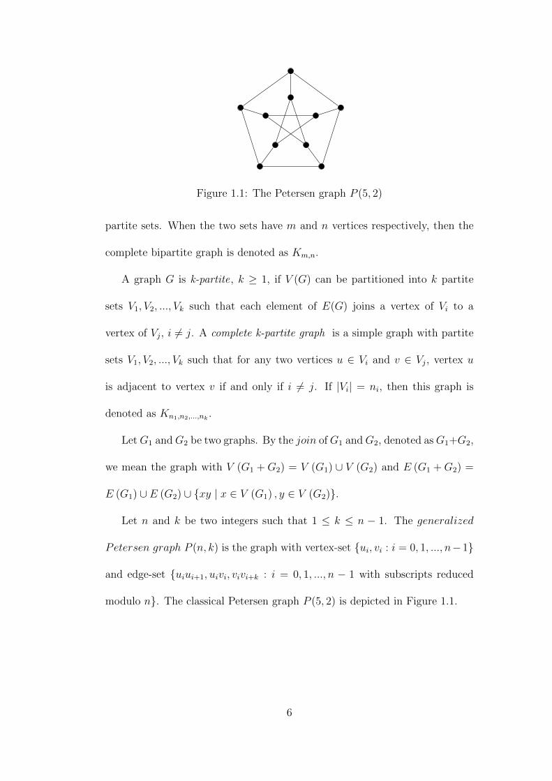
Figure 1.1: The Petersen graph P (5, 2)

partite sets. When the two sets have m and n vertices respectively, then the

complete bipartite graph is denoted as Km,n.

A graph G is k-partite, k ≥ 1, if V (G) can be partitioned into k partite

sets V1, V2, ..., Vk such that each element of E(G) joins a vertex of Vi to a

vertex of Vj, i 6= j. A complete k-partite graph is a simple graph with partite

sets V1, V2, ..., Vk such that for any two vertices u ∈ Vi and v ∈ Vj, vertex u

is adjacent to vertex v if and only if i 6= j. If |Vi| = ni, then this graph is

denoted as Kn1,n2,...,nk.

LetG1 andG2 be two graphs. By the join ofG1 andG2, denoted asG1+G2,

we mean the graph with V (G1 +G2) = V (G1) ∪ V (G2) and E (G1 +G2) =

E (G1) ∪ E (G2) ∪ {xy | x ∈ V (G1) , y ∈ V (G2)}.

Let n and k be two integers such that 1 ≤ k ≤ n − 1. The generalized

Petersen graph P (n, k) is the graph with vertex-set {ui, vi : i = 0, 1, ..., n−1}

and edge-set {uiui+1, uivi, vivi+k : i = 0, 1, ..., n − 1 with subscripts reduced

modulo n}. The classical Petersen graph P (5, 2) is depicted in Figure 1.1.

6

Chapter 2

Crossing Number

2.1 Introduction

The study of crossing numbers began during the Second World War with Paul

Turan’s brick factory problem that dates back as far as 1944. During the

Second World War, Turan was forced to work in a brick factory, using hand-

pulled carts that ran on tracks to move bricks from kilns to stores. When

tracks crossed, several bricks fell from the carts and had to be replaced by

hand.

So, a question arises, see [39]: what are the minimum number of crossings

of these tracks from kilns to stores? The problem, when formulated into graph

theory, is to find the crossing number of the complete bipartite graph Km,n.

In October 1952, Turan communicated the brick factory problem to other

mathematicians during his first visit to Poland. Solutions were then published

7

by topologist Zarankiewicz in 1954, see [44]. Years later, in 1968, Guy [12]

pointed out an error in Zarankiewicz’s proof and hence his formula yields only

an upper bound for the minimum number of crossings in complete bipartite

graphs. Many mathematicians have investigated Zarankiewicz’s conjecture on

the crossing number of complete bipartite graph. To date, in general, the long

standing Zarankiewicz’s conjecture has not been proved or disproved.

2.2 Crossing Number of Some Families of

Graphs

The investigation on the crossing number of graphs is a very difficult problem.

Despite much effort by many people, exact formulas of crossing numbers are

known only for relatively few graphs. To date, mathematicians still do not

know the exact value of the crossing numbers for basic graphs such as the

complete graph and the complete bipartite graph. In fact, finding the crossing

number of a given graph is a difficult task. In [10], Garey and Johnson have

shown that the problem of determining the crossing numbers of graphs is NP-

complete.

This section highlights some recent developments of crossing numbers of

graphs. In addition, some known good drawings of these families of graphs are

also given.

8

2.2.1 Complete Bipartite Graphs

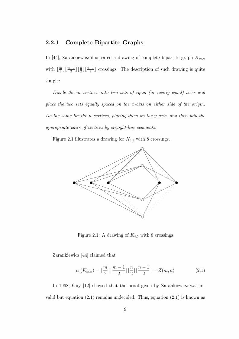
In [44], Zarankiewicz illustrated a drawing of complete bipartite graph Km,n

with bm2cbm−1

2cbn

2cbn−1

2c crossings. The description of such drawing is quite

simple:

Divide the m vertices into two sets of equal (or nearly equal) sizes and

place the two sets equally spaced on the x-axis on either side of the origin.

Do the same for the n vertices, placing them on the y-axis, and then join the

appropriate pairs of vertices by straight-line segments.

Figure 2.1 illustrates a drawing for K4,5 with 8 crossings.

Figure 2.1: A drawing of K4,5 with 8 crossings

Zarankiewicz [44] claimed that

cr(Km,n) = bm2cbm− 1

2cbn

2cbn− 1

2c = Z(m,n) (2.1)

In 1968, Guy [12] showed that the proof given by Zarankiewicz was in-

valid but equation (2.1) remains undecided. Thus, equation (2.1) is known as

9

Zarankiewicz’s Conjecture. However, some partial results are known. To date,

it has been proved that the conjecture is true for min{m,n} ≤ 6, by Kleitman

[20], and for the special cases 2 ≤ m ≤ 8, and 7 ≤ n ≤ 10, by Woodall [42].

Kleitman [20] also obtained the following lower bound of cr(Km,n) for

m ≥ 5.

cr(Km,n) ≥ 1

5m(m− 1)bn

2cbn− 1

2c (2.2)

In 2003, Nahas [32] improved the above lower bound for sufficiently large

m and n, and stated the new bound as follows:

cr(Km,n) ≥ 1

5m(m− 1)bn

2cbn− 1

2c+ 9.9× 10−6m2n2 (2.3)

In 2006, Klerk, Maharry, Pasechnik, Richter and Salazar, see [21], showed

that, for m ≥ 9, limn→∞cr(Km,n)

Z(m,n)≥ α m

m−1 where α = 0.83. The authors in [22]

then strengthened the result by improving α to 0.8594.

2.2.2 Complete Graphs

In 1960, Guy [11] obtained an upper bound on the crossing number for the

complete graph Kn.

cr (Kn) ≤ 1

4bn

2cbn− 1

2cbn− 2

2cbn− 3

2c (2.4)

.

Figure 2.2 shows drawings of complete graphs K5 and K6 with one and

three crossings respectively.

10

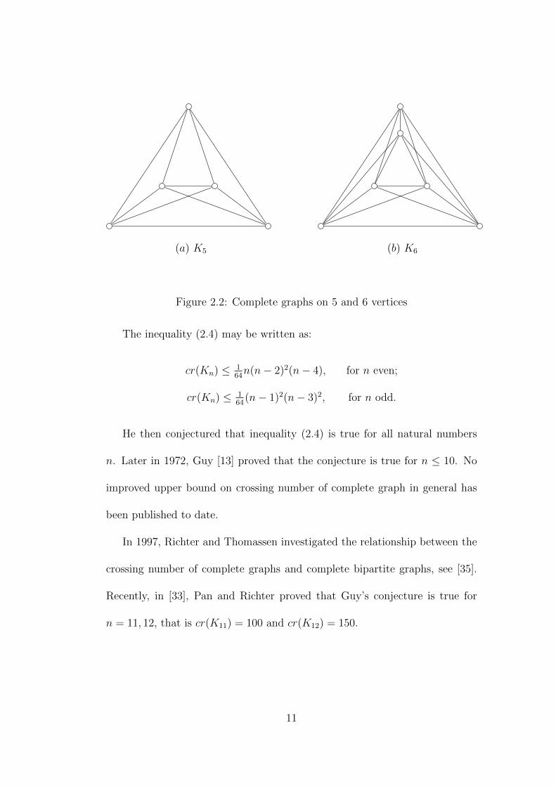
(a) K5 (b) K6

Figure 2.2: Complete graphs on 5 and 6 vertices

The inequality (2.4) may be written as:

cr(Kn) ≤ 164n(n− 2)2(n− 4), for n even;

cr(Kn) ≤ 164

(n− 1)2(n− 3)2, for n odd.

He then conjectured that inequality (2.4) is true for all natural numbers

n. Later in 1972, Guy [13] proved that the conjecture is true for n ≤ 10. No

improved upper bound on crossing number of complete graph in general has

been published to date.

In 1997, Richter and Thomassen investigated the relationship between the

crossing number of complete graphs and complete bipartite graphs, see [35].

Recently, in [33], Pan and Richter proved that Guy’s conjecture is true for

n = 11, 12, that is cr(K11) = 100 and cr(K12) = 150.

11

2.2.3 Complete Tripartite Graphs

As for the crossing number of the complete tripartite graph Kl,m,n, to date,

there are only a few results for the case where both l and m are small values.

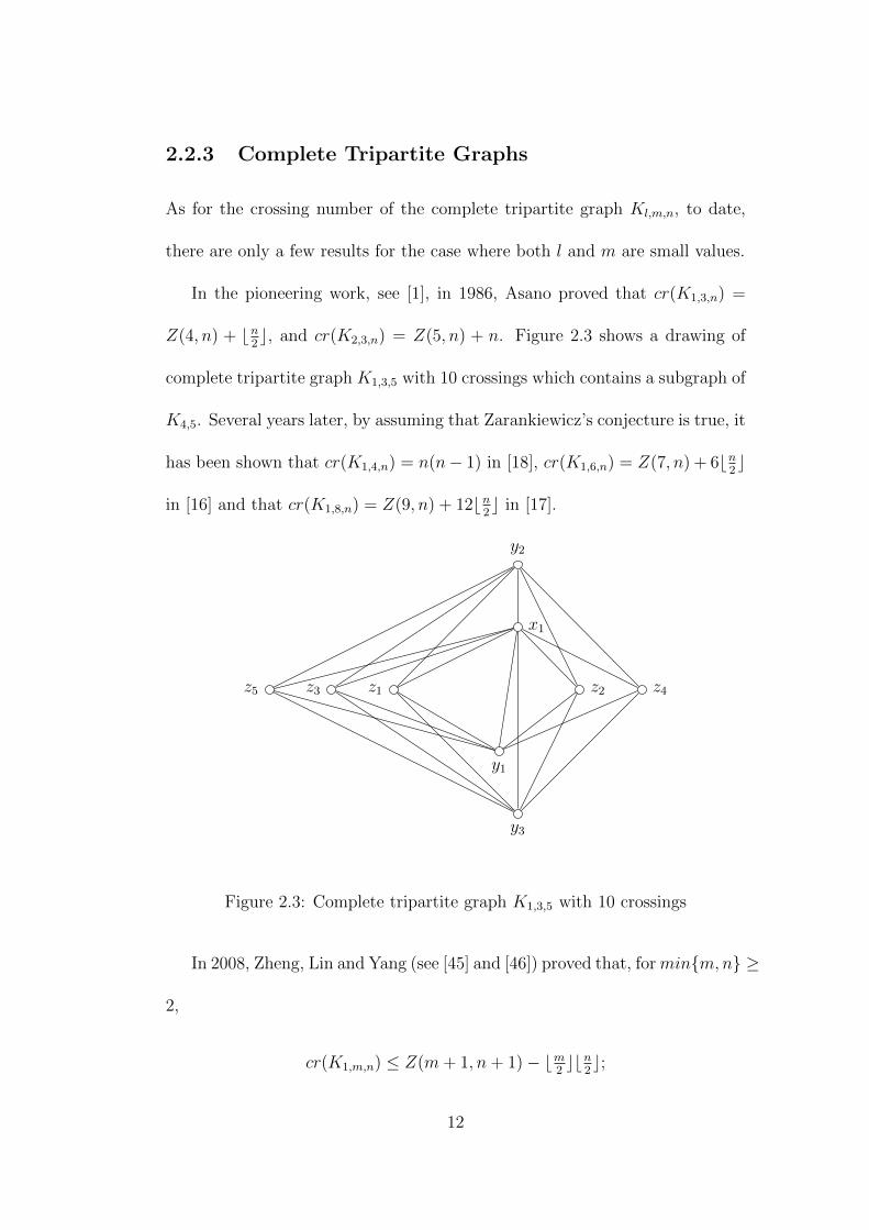
In the pioneering work, see [1], in 1986, Asano proved that cr(K1,3,n) =

Z(4, n) + bn2c, and cr(K2,3,n) = Z(5, n) + n. Figure 2.3 shows a drawing of

complete tripartite graph K1,3,5 with 10 crossings which contains a subgraph of

K4,5. Several years later, by assuming that Zarankiewicz’s conjecture is true, it

has been shown that cr(K1,4,n) = n(n− 1) in [18], cr(K1,6,n) = Z(7, n) + 6bn2c

in [16] and that cr(K1,8,n) = Z(9, n) + 12bn2c in [17].

z5 z3 z1 z2 z4

y3

x1

y2

y1

Figure 2.3: Complete tripartite graph K1,3,5 with 10 crossings

In 2008, Zheng, Lin and Yang (see [45] and [46]) proved that, formin{m,n} ≥

2,

cr(K1,m,n) ≤ Z(m+ 1, n+ 1)− bm2cbn

2c;

12

cr(K2,m,n) ≤ Z(m+ 2, n+ 2)−mn.

The equalities hold for min{m,n} ≤ 3 in both cases. Zheng, Lin and Yang

in [45] then conjectured that it is true in general.

Later, in 2008, Ho [15] obtained a lower bound of the crossing number of

complete tripartite graph, which is cr(K1,m,n) ≥ cr(Km+1,n+1)−b nmbm2cbm+1

2cc

by constructing drawings of Km+1,n+1 which preserve all the optimality from

a good drawing of K1,m,n. Ho [15] showed that the equality holds for m = 4.

In fact, due to the complexity of complete tripartite graphs, especially

with bigger value of the order of each partite set, no further results on crossing

number of complete tripartite graphs has been obtained.

2.2.4 Join of Graphs

In 2007, Klesc gave the exact values of crossing numbers for the join of two

paths, the join of two cycles, and for the join of path and cycle, see [23].

Theorem 2.1 [23]

(a) cr(Pm + Pn) = Z(m,n) for min {m,n} ≤ 6;

(b) cr(Pm+Cn) = Z(m,n)+1 for any m ≥ 2, n≥ 3 with min{m,n} ≤ 6;

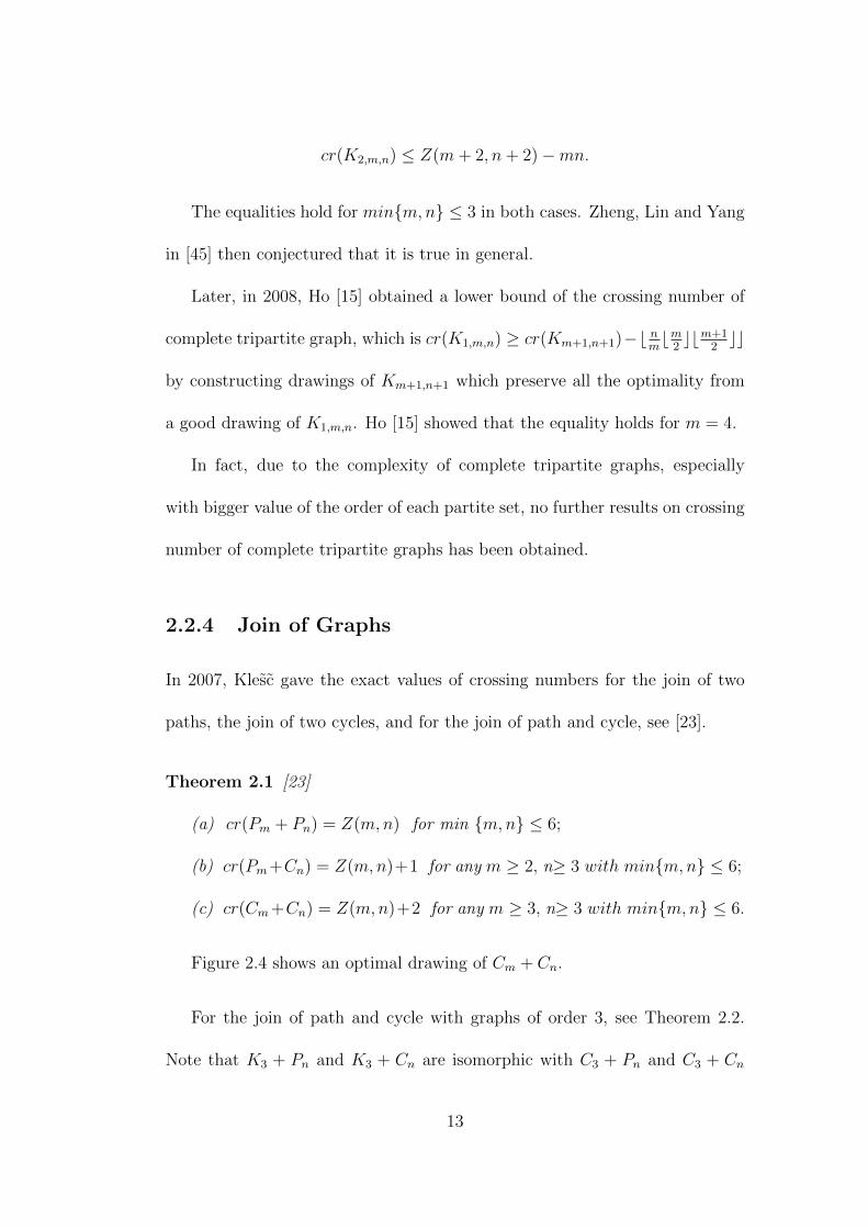
(c) cr(Cm+Cn) = Z(m,n)+2 for any m ≥ 3, n≥ 3 with min{m,n} ≤ 6.

Figure 2.4 shows an optimal drawing of Cm + Cn.

For the join of path and cycle with graphs of order 3, see Theorem 2.2.

Note that K3 + Pn and K3 + Cn are isomorphic with C3 + Pn and C3 + Cn

13

Figure 2.4: The graph Cm + Cn

respectively. Thus the crossing numbers of these graphs follows from Theorem

2.1.

Theorem 2.2 [23] For n ≥ 3, cr(3K1 +Pn) = cr((K1∪P2) +Pn) = cr(3K1 +

Cn) = cr((K1 ∪ P2) + Cn) = Z(3, n).

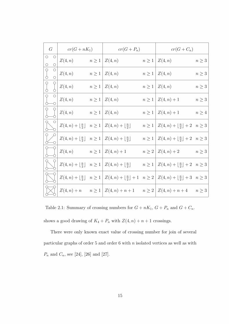
In [23], Klesc extended the results in Theorem 2.1 to the join products

G+Pn and G+Cn where G is a graph with order at most 4. Table 2.1 shows

a summary of the crossing numbers for the join products of path, cycle and

n isolated vertices with all graphs G of order four, see [23] and [25]. Both

connected and disconnected graphs of G are taken into account. Figure 2.5

14

G cr(G+ nK1) cr(G+ Pn) cr(G+ Cn)

Z(4, n) n ≥ 1 Z(4, n) n ≥ 1 Z(4, n) n ≥ 3

Z(4, n) n ≥ 1 Z(4, n) n ≥ 1 Z(4, n) n ≥ 3

Z(4, n) n ≥ 1 Z(4, n) n ≥ 1 Z(4, n) n ≥ 3

Z(4, n) n ≥ 1 Z(4, n) n ≥ 1 Z(4, n) + 1 n ≥ 3

Z(4, n) n ≥ 1 Z(4, n) n ≥ 1 Z(4, n) + 1 n ≥ 4

Z(4, n) + bn2c n ≥ 1 Z(4, n) + bn

2c n ≥ 1 Z(4, n) + bn

2c+ 2 n ≥ 3

Z(4, n) + bn2c n ≥ 1 Z(4, n) + bn

2c n ≥ 1 Z(4, n) + bn

2c+ 2 n ≥ 3

Z(4, n) n ≥ 1 Z(4, n) + 1 n ≥ 2 Z(4, n) + 2 n ≥ 3

Z(4, n) + bn2c n ≥ 1 Z(4, n) + bn

2c n ≥ 1 Z(4, n) + bn

2c+ 2 n ≥ 3

Z(4, n) + bn2c n ≥ 1 Z(4, n) + bn

2c+ 1 n ≥ 2 Z(4, n) + bn

2c+ 3 n ≥ 3

Z(4, n) + n n ≥ 1 Z(4, n) + n+ 1 n ≥ 2 Z(4, n) + n+ 4 n ≥ 3

Table 2.1: Summary of crossing numbers for G+ nK1, G+ Pn and G+ Cn.

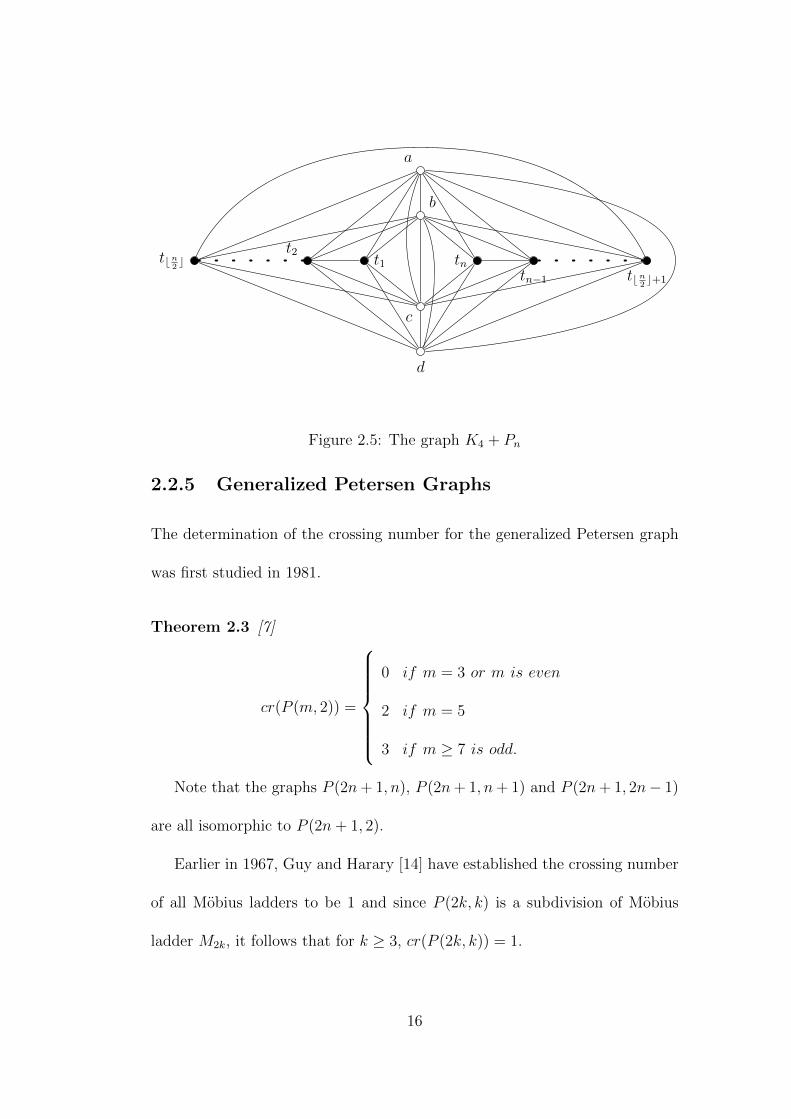
shows a good drawing of K4 + Pn with Z(4, n) + n+ 1 crossings.

There were only known exact value of crossing number for join of several

particular graphs of order 5 and order 6 with n isolated vertices as well as with

Pn and Cn, see [24], [26] and [27].

15

tbn2c

t2t1 tn

tn−1 tbn2c+1

d

c

b

a

Figure 2.5: The graph K4 + Pn

2.2.5 Generalized Petersen Graphs

The determination of the crossing number for the generalized Petersen graph

was first studied in 1981.

Theorem 2.3 [7]

cr(P (m, 2)) =

0 if m = 3 or m is even

2 if m = 5

3 if m ≥ 7 is odd.

Note that the graphs P (2n+ 1, n), P (2n+ 1, n+ 1) and P (2n+ 1, 2n− 1)

are all isomorphic to P (2n+ 1, 2).

Earlier in 1967, Guy and Harary [14] have established the crossing number

of all Mobius ladders to be 1 and since P (2k, k) is a subdivision of Mobius

ladder M2k, it follows that for k ≥ 3, cr(P (2k, k)) = 1.

16

In 1986, Fiorini [8] proved that P (8, 3) has crossing number 4 and claimed

that P (10, 3) also has crossing number 4. Years later, in [31], McQuillan

and Richter gave a short proof of the first claim and showed that the second

claim is false. Then, again, Richter and Sazalar [34] found a gap in some

of Fiorini’s proofs which invalidated his principal results about cr(P (n, 3)).

However, Fiorini has shown the following.

Theorem 2.4 [8]

(i) cr(P(8,3)) = 4

(ii) cr(P(9,3)) = 2

(iii) cr(P(12,3)) = 4

In 1997, Sarazin [37] proved the following.

Theorem 2.5 [37] cr(P (10, 4)) = 4.

In 2002, Richter and Sazalar [34] determined the crossing number of P (3k+

h, 3).

Theorem 2.6 [34]

cr(P (3k + h, 3)) =

k + h if h ∈ {0, 2}

k + 3 if h = 1.

for each k ≥ 3, with the single exception of P (9, 3) where cr(P (9, 3)) = 2.

17

In 2003, Fiorini and Gausi [9] determined the crossing number of P (3k, k)

(see [8] and [34]) and showed that cr(P (3k, k)) = k. However, Chia and Lee

[4] pointed out a flaw in the proof in [9], and provided a correct proof.

In 2013, Yang, Zheng and Xu [43] proved that cr(P (10, 3)) = 6.

To date, the crossing numbers of other generalized Petersen graphs remain

unknown.

2.3 Planarity Criterion

Planarity being such a fundamental property, the problem of deciding whether

a given graph is planar is remarkably important. There is a simple formula

relating the number of vertices, edges, and faces in a connected plane graph.

It was first established for polyhedral graphs by Euler (1752), and is known as

Euler’s Formula.

Theorem 2.7 (Euler’s Formula) Let G be a connected plane graph with p

vertices, q edges and f faces. Then

p− q + f = 2.

Euler’s formula can easily be extended to disconnected graph. For plane

graphs in general, we have the following.

Corollary 2.8 Let G be a plane graph with p vertices, q edges, f faces and k

components. Then

p− q + f = 1 + k.

18

Note that in any graph, the sum of the vertex degrees is equal to twice the

number of edges. This is called the Hand-shaking Lemma.

An immediate consequence is the following.

Corollary 2.9 Let G be a planar graph with q edges, f faces and girth g.

Then

2q ≥ gf .

By Theorem 2.7 and Collorary 2.9, we have the following.

Corollary 2.10 Let G be a simple connected planar graph with p vertices and

q edges, p ≥ 3. Then q ≤ 3p− 6. Furthermore, q = 3p− 6 if and only if G is

a maximal planar graph.

For the case where a plane graph G contains no triangle, the girth of G is at

least 4. Hence by Theorem 2.7 and Collorary 2.9 again, we have the following

theorem.

Theorem 2.11 Suppose G is a planar graph containing no triangle, having p

vertices and q edges, p ≥ 3. Then

q ≤ 2p− 4.

An important consequence of Colloraries 2.9 and 2.10 is the following.

Theorem 2.12 K3,3 and K5 are non-planar.

19

K3,3 and K5 are important in determining the planarity of a graph. The

most well known characterization of planar graphs is the Kuratowski’s Theo-

rem.

Theorem 2.13 (Kuratowski’s Theorem). A graph is planar if and only if it

contains no subgraph which is a subdividion of K5 or K3,3.

2.4 Crossing-critical Graphs

2.4.1 Definitions

A graph G is said to be crossing-critical if deleting any edge decreases its

crossing number on the plane, that is cr(G− e) < cr(G) for every edge e of G.

Let Fn(cr) denote the family of crossing-critical graphs G, where cr(G) > n

and cr(G − e) ≤ n for every edge e of G and no vertex of G has degree two.

For every graph H, cr(H) ≤ n if and only if H does not contain a subgraph

homeomorphic to a member of Fn(cr). Clearly, Fn(cr) is a family of some

“forbidden subgraphs” of graph H with cr(H) ≤ n.

2.4.2 Some Ideas and Examples

From Theorem 2.13, we conclude that the members of F0(cr) are K5 and K3,3.

Now, a question arises: For every n ≥ 1, is Fn(cr) a finite set?

Note that there exists infinitely many 2-connected graphs of Fn(cr) for

every n ≥ 1, see Figure 2.6. Then, the following question is of some interest:

20

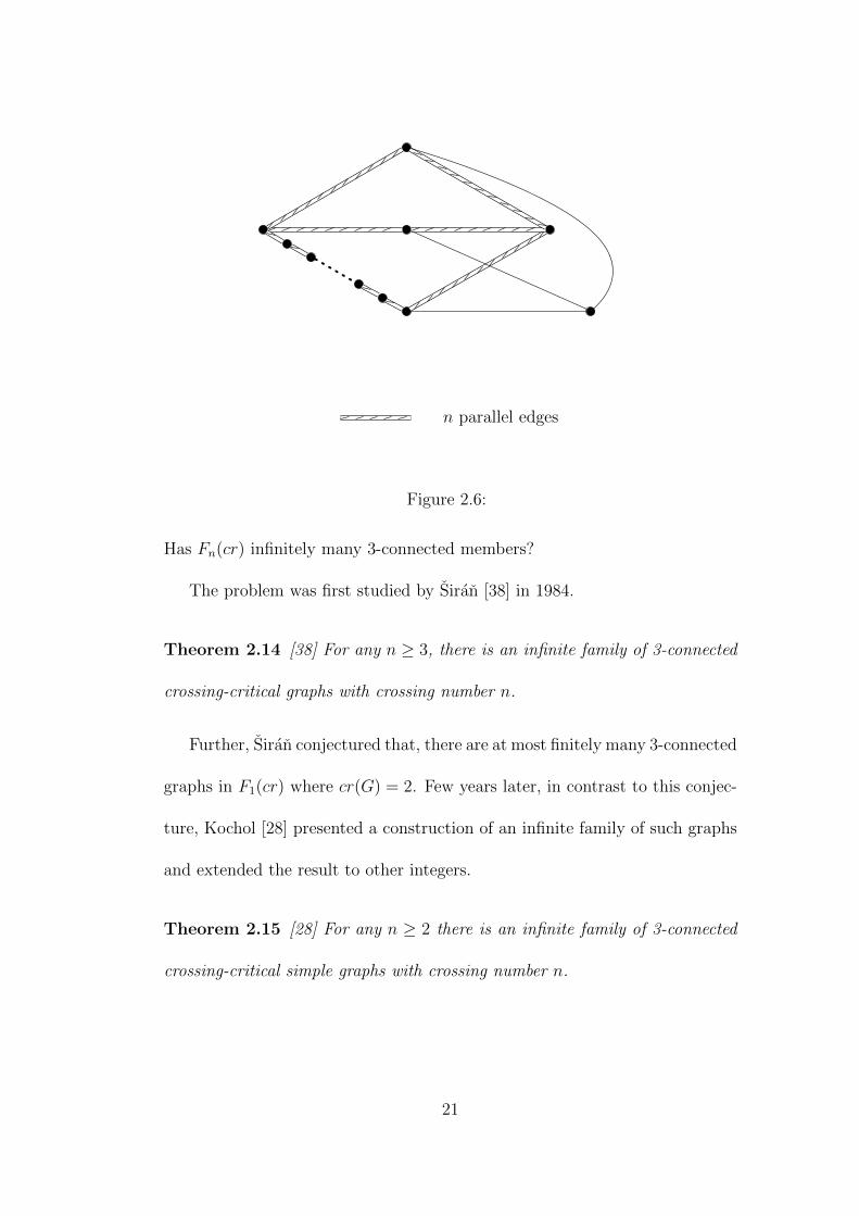
n parallel edges

Figure 2.6:

Has Fn(cr) infinitely many 3-connected members?

The problem was first studied by Siran [38] in 1984.

Theorem 2.14 [38] For any n ≥ 3, there is an infinite family of 3-connected

crossing-critical graphs with crossing number n.

Further, Siran conjectured that, there are at most finitely many 3-connected

graphs in F1(cr) where cr(G) = 2. Few years later, in contrast to this conjec-

ture, Kochol [28] presented a construction of an infinite family of such graphs

and extended the result to other integers.

Theorem 2.15 [28] For any n ≥ 2 there is an infinite family of 3-connected

crossing-critical simple graphs with crossing number n.

21

Chapter 3

Skewness of Graphs

3.1 Introduction

Similar to crossing number, skewness of graphs could be thought of as a mea-

sure of how non-planar a graph is. Graph operations such as vertex deletion,

vertex splitting and edge deletion have been widely studied (see [29]) in mak-

ing a non-planar graph into a planar one. While it is hard to find the crossing

numbers for the complete graphs, the complete bipartite graphs and the join

of graphs, the determination of skewness of these graphs turns out to be not

too difficult (see [6] and [29]).

In this section, we are more concerned with the edge deletion operation,

a topic that has been studied intensively and that has many applications in

VSLI circuit routing. It is also associated with the Maximum Planar Subgraph

Problem (see [29] for more details).

22

In [29], Liebers suggested the following definition on skewness of graphs.

Definition 3.1 (maximum planar subgraph, skewness) If a graph G′ = (V,E ′)

is a planar subgraph of a graph G = (V,E) such that there is no planar subgraph

G′′ = (V,E ′′) of G with |E ′′| > |E ′|, then G′ is called a maximum planar

subgraph of G, and the number of deleted edges, |E|−|E ′| is called the skewness

of G.

In short, the skewness of a graphG, denoted sk(G), is the minimum number

of edges in G whose deletion results in a planar graph. It is clear that sk(G) ≤

cr(G). [30] shows that the problem of determining the skewness of a graph is

NP-complete.

3.2 π − skewness

In this section, we provide some elementary facts about skewness of graphs

and introduce the definition of π − skew graph.

Remark 3.2 (i) sk(G) = 0 if and only if G is a planar graph.

(ii) If two graphs G1 and G2 are homeomorphic, then sk(G1) = sk(G2).

(iii) If H is a subgraph of a graph G, then sk(H) ≤ sk(G).

(iv) If there is a planar graph H which can be obtained by deleting r edges

from the graph G, then sk(G) ≤ r.

(v) sk(G) = 1 if cr(G) = 1.

23

Recalling that cr(K5) = 1 and cr(K3,3) = 1. By Remark 3.2 (v), we can

conclude that sk(K5) = 1 and sk(K3,3) = 1.

Euler’s formula (Theorem 2.7) together with the Hand-shaking Lemma

(Corollary 2.9) yield the following.

Theorem 3.3 Let G be a graph on p vertices, q edges and having girth g. If

G is planar, then

q ≤ gg−2(p− 2).

Hence, we have the following.

Theorem 3.4 Let G be a graph on p vertices, q edges and having girth g.

Then

sk(G) ≥ q − gg−2(p− 2).

One natural thing to ask is: When does equality holds?

Definition 3.5 Let G be a graph on p vertices, q edges and having girth g.

Define

π(G) = dq − gg−2(p− 2)e.

Note that the general form of this combinatorial invariant appeared in [19].

We say that the graph G is π − skew if sk(G) = π(G).

Theorem 3.6 For any connected graph G, we have sk(G)≥ π(G).

24

3.3 Known Results

We now turn our attention to some known results on the skewness of some

families of graphs.

Proposition 3.7 Suppose G is the complete graph Kn. Then sk(G) = π(G) =(n−32

).

Proposition 3.8 [4] Let m,n ≥ 2. Then sk(Km,n) = π(Km,n) = (m− 2)(n−

2).

Now, we give a short proof for sk(Km,n) = π(Km,n). By Theorem 3.6,

we have sk(Km,n) ≥ π(Km,n). It remains to prove that there exists a planar

graph by removing (m−2)(n−2) (which is equal to π(Km,n)) edges from Km,n.

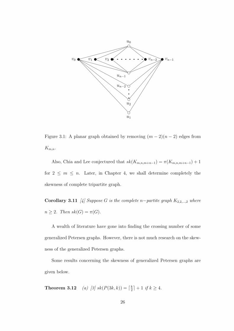
Figure 3.1 shows a planar subgraph of Km,n after deleting (m−2)(n−2) edges.

Hence, Km,n is π − skew. Note that a complete bipartite graph is of girth 4.

In [4], Chia and Lee gave some partial results on skewness of complete

tripartite graph Km,n,t.

Proposition 3.9 [4] Suppose n ≤ t and G is the graph K1,n,t. Then sk(G) =

π(G) + t− 1.

Proposition 3.10 [4] Suppose m,n and t are integers such that 2 ≤ m ≤ n ≤

t where t ≤ m + n − 2. Let G be the complete tripartite graph Km,n,t. Then

sk(G) = π(G).

25

v0 v1 v2 vn−2 vn−1

u1

u2

un−2

un−1

u0

Figure 3.1: A planar graph obtained by removing (m − 2)(n − 2) edges from

Km,n.

Also, Chia and Lee conjectured that sk(Km,n,m+n−1) = π(Km,n,m+n−1) + 1

for 2 ≤ m ≤ n. Later, in Chapter 4, we shall determine completely the

skewness of complete tripartite graph.

Corollary 3.11 [4] Suppose G is the complete n−partite graph K2,2,...,2 where

n ≥ 2. Then sk(G) = π(G).

A wealth of literature have gone into finding the crossing number of some

generalized Petersen graphs. However, there is not much research on the skew-

ness of the generalized Petersen graphs.

Some results concerning the skewness of generalized Petersen graphs are

given below.

Theorem 3.12 (a) [3] sk(P (3k, k)) = dk2e+ 1 if k ≥ 4.

26

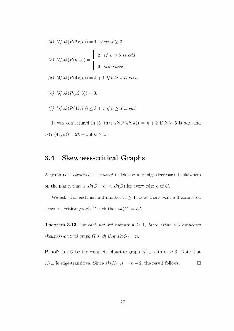
(b) [4] sk(P (2k, k)) = 1 where k ≥ 3.

(c) [4] sk(P (k, 2)) =

2 if k ≥ 5 is odd

0 otherwise.

(d) [5] sk(P (4k, k)) = k + 1 if k ≥ 4 is even.

(e) [5] sk(P (12, 3)) = 3.

(f) [5] sk(P (4k, k)) ≤ k + 2 if k ≥ 5 is odd.

It was conjectured in [5] that sk(P (4k, k)) = k + 2 if k ≥ 5 is odd and

cr(P (4k, k)) = 2k + 1 if k ≥ 4.

3.4 Skewness-critical Graphs

A graph G is skewness − critical if deleting any edge decreases its skewness

on the plane, that is sk(G− e) < sk(G) for every edge e of G.

We ask: For each natural number n ≥ 1, does there exist a 3-connected

skewness-critical graph G such that sk(G) = n?

Theorem 3.13 For each natural number n ≥ 1, there exists a 3-connected

skewness-critical graph G such that sk(G) = n.

Proof: Let G be the complete bipartite graph K3,m with m ≥ 3. Note that

K3,m is edge-transitive. Since sk(K3,m) = m− 2, the result follows.

27

Chapter 4

Skewness of the Join of Graphs

4.1 Introduction

Suppose G is a graph with p vertices and having girth g. If G is π-skew, then

G contains a planar subgraph H with p vertices and d gg−2(p − 2)e edges. In

particular, if G is π-skew and is of girth 3, then H is a spanning maximal

planar subgraph of G. Besides complete graph and complete bipartite graph,

another example of a π-skew graph is given by the n−cube whose skewness

has been determined in [6].

Theorem 4.1 Suppose that G is a complete graph or a complete bipartite

graph. Then G is π-skew.

In the rest of the sections, we determine completely the skewness of the

complete k−partite graphs for k = 3, 4. This is done by first establishing some

results concerning the skewness for the join of two graphs and then applying

28

the results on the complete multipartite graphs.

4.2 Join of Graphs

Lemma 4.2 For each i = 1, 2, let Gi be a connected graph on pi vertices.

Then

sk(G1 +G2) ≥ sk(G1) + sk(G2) + (p1 − 2)(p2 − 2).

Proof: Note that G1 + G2 contains a subgraph Kp1,p2 whose skewness is

π(Kp1,p2) = (p1 − 2)(p2 − 2) by Theorem 4.1. In order to obtain a spanning

planar subgraph of G1 +G2, we need to delete at least sk(G1) edges from G1,

at least sk(G2) edges from G2, and at least (p1 − 2)(p2 − 2) from Kp1,p2 . But

this means that sk(G1 + G2) ≥ sk(G1) + sk(G2) + (p1 − 2)(p2 − 2), and the

lemma follows.

A direct consequence is the following. Let Kn denote the complement of

the complete graph with n vertices.

Corollary 4.3 Let G be a connected graph on p vertices. Then

sk(G+Ks) ≥ sk(G) + (p− 2)(s− 2).

We shall now introduce two techniques, which we call vertex triangulation

of a face and building faces on a given edge. These techniques will be used

throughout the rest of the sections.

29

Definition 4.4 Let H denote a plane graph. (i) Let F denote a face of H.

By a vertex triangulation of F , we mean inserting a new vertex x inside F and

joining x to each vertex of F . (ii) Let uv be an edge of H. By building a fetch

on uv with a new vertex x we mean joining x to u and v.

Theorem 4.5 Let G be a connected graph on p vertices with girth 3. Suppose

sk(G) = π(G). Then for any positive integer s,

sk(G+Ks) =

π(G+Ks) if s ≤ 2p− 4

π(G+Ks) + s− 2p+ 4 otherwise.

Proof: Since G is of girth 3, π(G) = |E(G)|−3(p−2). Because sk(G) = π(G),

we have |E(G)|−sk(G) = 3(p−2), and this means that there exists a maximal

planar subgraph H of G with p vertices and 3(p− 2) edges.

Draw H on the plane with no crossings. Note that H has 2p− 4 faces, and

that each face is a triangle.

If s ≤ 2p−4, we can add s new vertices, one inside each face of H, and join

each new vertex v to the three vertices on the face containing v. The result

is a maximal planar subgraph of G + Ks on p + s vertices. This proves that

sk(G+Ks) = π(G+Ks).

Hence assume that s ≥ 2p− 4, and write t = s− 2(p− 2). We shall show

that sk(G+Ks) = π(G+Ks) + t.

By Corollary 4.3, sk(G+Ks) ≥ sk(G) + (p− 2)(s− 2), and it is routine to

check that sk(G) + (p− 2)(s− 2) = π(G+Ks) + t.

30

To show that sk(G+Ks) ≤ π(G+Ks) + t, we do the following.

Consider the plane subgraph H of G (from the second paragraph) and

vertex-triangulate each of the 2p − 4 faces of H. We then build fetches on a

fixed edge of H with each of the remaining t = s−2p+4 vertices. The resulting

graph J is planar, and clearly has p+s vertices and 3(2p−4) + 3(p−2) + 2t =

9(p−2)+2t = 5(p−2)+2s edges, which means that sk(G+Ks) ≤ π(G+Ks)+t.

This completes the proof.

Theorem 4.5 can be used to generate infinitely many π−skew graphs re-

cursively. Since G+Ks is of girth 3 if s ≤ 2p− 4, it follows from Theorem 4.5

that (G+Ks)+Kr is π−skew if r ≤ 2(p+s)−4. This process can be repeated

to generate π−skew graphs of the form G + Km1,m2,...,mr where m1 ≤ 2p − 4

and mi ≤ 2(p+m1 + ...+mi−1)− 4 for each i = 2, ..., r.

One may ask: To what extent can the conditions on G in Theorem 4.5 be

relaxed and we still get π−skewness in G + Ks? We do not know the answer

in general. Some special cases are considered in the next section.

4.3 Complete Tripartite Graphs

If a graph G with p vertices has girth 4, then it is not true in general that

sk(G) = π(G) implies that sk(G+Ks) = π(G+Ks) if s ≤ p−2. For example,

take G to be the 4-cycle and s = 1; then sk(G+Ks) = 0, but π(G+Ks) < 0.

However, for the special case when G is the complete bipartite graph Km,n,

where 2 ≤ m ≤ n, it has been shown in [4] that sk(G + Ks) = π(G + Ks) if

31

n ≤ s ≤ m + n − 2. Note that Km,n + Ks = Km,n,s. Also, it has been shown

in [4] that, if H ∼= Km,n,m+n−1, then π(H) ≤ sk(H) ≤ π(H) + 1. Also, it

was believed that sk(H) = π(H) + 1. We shall now determine completely the

skewness of Km,n,r with the use of Theorem 4.5. Here, a much easier proof

(than the one given in [4]) for the case n ≤ s ≤ m+ n− 2 is also provided.

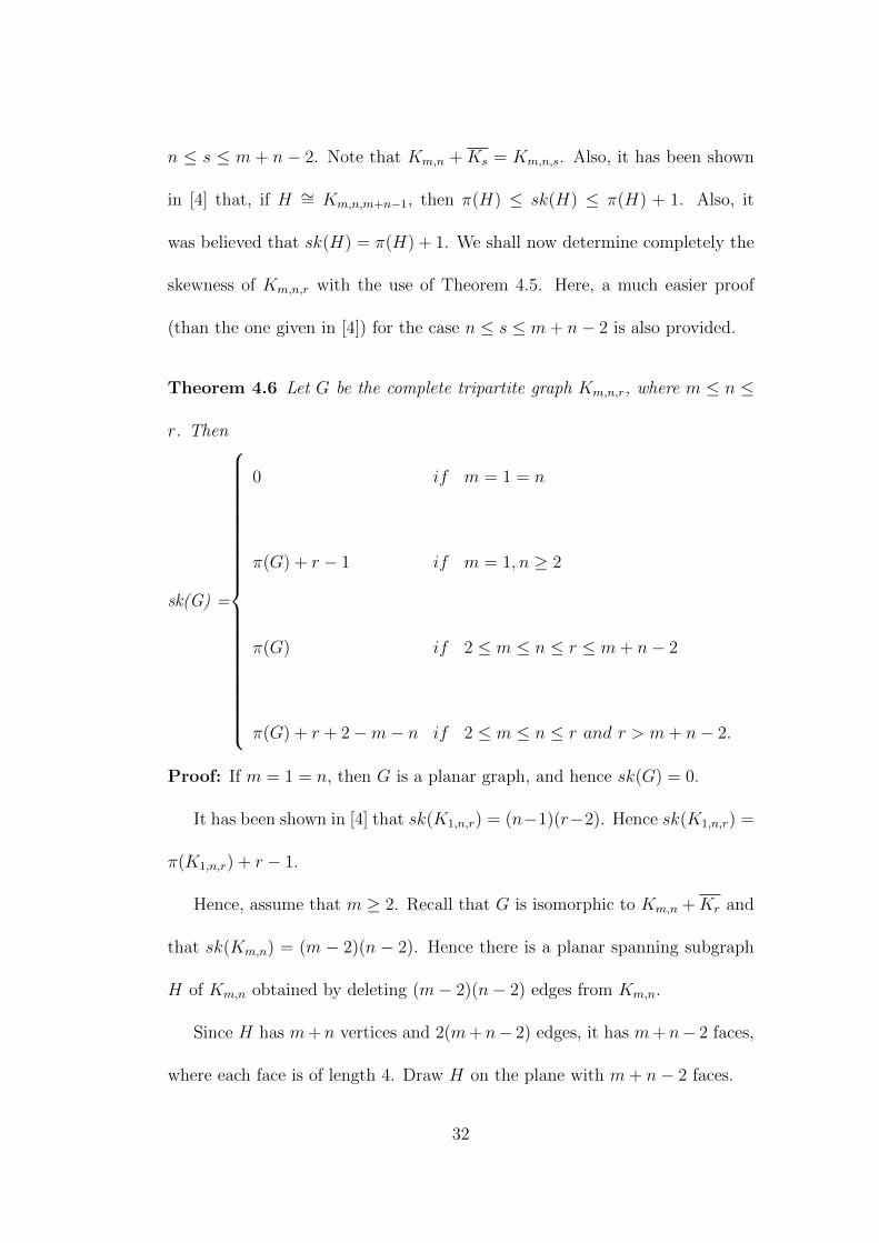
Theorem 4.6 Let G be the complete tripartite graph Km,n,r, where m ≤ n ≤

r. Then

sk(G) =

0 if m = 1 = n

π(G) + r − 1 if m = 1, n ≥ 2

π(G) if 2 ≤ m ≤ n ≤ r ≤ m+ n− 2

π(G) + r + 2−m− n if 2 ≤ m ≤ n ≤ r and r > m+ n− 2.

Proof: If m = 1 = n, then G is a planar graph, and hence sk(G) = 0.

It has been shown in [4] that sk(K1,n,r) = (n−1)(r−2). Hence sk(K1,n,r) =

π(K1,n,r) + r − 1.

Hence, assume that m ≥ 2. Recall that G is isomorphic to Km,n +Kr and

that sk(Km,n) = (m − 2)(n − 2). Hence there is a planar spanning subgraph

H of Km,n obtained by deleting (m− 2)(n− 2) edges from Km,n.

Since H has m+n vertices and 2(m+n− 2) edges, it has m+n− 2 faces,

where each face is of length 4. Draw H on the plane with m+ n− 2 faces.

32

Assume first that r > m+n−2, and write r = m+n−2+t for some integer

t > 0. Then vertex-triangulate each face of H and follow this by building t

fetches on a fixed edge of H. The resulting planar graph J is a spanning

subgraph of G, and |E(J)| = 2(m + n − 2) + 4(m + n − 2) + 2(r −m − n +

2) = 4(m + n − 2) + 2r. This means that sk(G) ≤ |E(G)| − |E(J)|. Since

π(G) = |E(G)| − 3(m+ n+ r − 2), we have sk(G) ≤ π(G) + r + 2−m− n.

On the other hand, by Corollary 4.3, sk(G) ≥ (m− 2)(n− 2) + (m+ n−

2)(r− 2). Clearly, (m− 2)(n− 2) + (m+n− 2)(r− 2) = π(G) + r+ 2−m−n.

This proves that sk(G) = π(G) + r + 2−m− n in this case.

Next, assume that r ≤ m + n − 2. To show that sk(G) = π(G), we just

need to show that there is a spanning maximal planar subgraph M of G. To

do this, we shall construct a plane graph Hm,n,r on m + n vertices having r

faces so that Hm,n,r is a subgraph of Km,n. Then, by vertex-triangulating every

face of Hm,n,r, we obtain the required planar graph M .

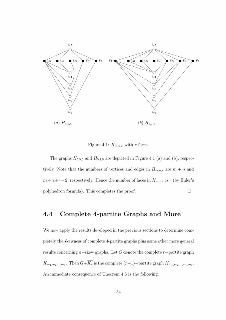
For this purpose, let V (Hm,n,r) = {u1, u2, ..., um, v1, v2, ..., vn}, where s =

n − m and t = r − n for some non-negative integers s and t. The edges of

Hm,n,r are as follows.

(i) umvi is an edge for all i = 1, 2, ..., n.

(ii) vnui is an edge for all i = 1, 2, ...,m.

(iii) uivi is an edge for all i = 1, 2, ...,m− 1.

(iv) um−1vi is an edge for every m− 1 ≤ i ≤ m− 1 + s.

(v) uivi−1 is an edge for every m− t ≤ i ≤ m− 1 if t ≥ 1.

33

u1

u2

u3

u4

u5

v1v2v3v4v5

u1

u2

u3

u4

u5

v1v2v3v4v5v6v7

(a) H5,5,5 (b) H5,7,9

Figure 4.1: Hm,n,r with r faces

The graphs H5,5,5 and H5,7,9 are depicted in Figure 4.1 (a) and (b), respec-

tively. Note that the numbers of vertices and edges in Hm,n,r are m + n and

m+n+r−2, respectively. Hence the number of faces in Hm,n,r is r (by Euler’s

polyhedron formula). This completes the proof.

4.4 Complete 4-partite Graphs and More

We now apply the results developed in the previous sections to determine com-

pletely the skewness of complete 4-partite graphs plus some other more general

results concerning π−skew graphs. Let G denote the complete r−partite graph

Km1,m2,...,mr . Then G+Ks is the complete (r+1)−partite graph Km1,m2,...,mr,ms .

An immediate consequence of Theorem 4.5 is the following.

34

Corollary 4.7 Suppose that the complete r-partite graph Km1,m2,...,mr is π −

skew, where r ≥ 3. Then so is the complete (r+1)-partite graph Km1,m2,...,mr,m

for any positive integer m ≤ 2(m1 +m2 + ...+mr)− 4.

In [4], it was shown that, if G is the complete r−partite graph K2,2,...,2,

where r ≥ 2, then G is π−skew. The following result generalizes this.

Corollary 4.8 Suppose G is the complete r−partite graph Kn,n,...,n where n ≥

1 and r ≥ 2. Then G is π−skew.

Proof: When n = 1, G is the complete graph Kr, and hence is π−skew. So

we may assume that n ≥ 2.

When r = 2, sk(G) = π(G) by Theorem 4.1. So we may assume that r ≥ 3.

When n = 2 and r = 3, we see that G is a maximal planar graph, and

hence is π−skew. By Corollary 4.7 and by induction on r, it follows that, if G

is the complete r−partite graph K2,2,...,2, then sk(G) = π(G).

So we may assume that n ≥ 3. By Theorems 4.1 and 4.6, Kn,n and Kn,n,n

are π−skew. By Corollary 4.7 and by induction on r, it follows that Kn,n,...,n

is π−skew.

By Corollary 4.8 and Theorem 4.5, we have the following.

Corollary 4.9 Suppose that G is the complete (r+1)−partite graph Kn,n,...,n,m

where n ≥ 1 and r ≥ 3. Then

35

sk(G)=

π(G) if m ≤ 2nr − 4

π(G) +m− 2nr + 4 otherwise.

Therefore it follows directly from Corollary 4.9 that sk(K1,1,1,m) is equal to

0 if m ≤ 2 and is equal to m− 2 otherwise.

Proposition 4.10 Let G be the complete 4-partite graph K1,1,m,n where 2 ≤

m ≤ n. Then

sk(G) =

π(G) if n ≤ m+ 1

π(G) + n−m− 1 otherwise.

Proof: Note that G ∼= K1,1,m +Kn and that K1,1,m can be drawn on the plane

with m+ 1 faces, where two of them are 3-faces and m−1 of them are 4-faces.

If we do a vertex-triangulation on each face followed by building fetches on

some fixed edge, the result follows.

A natural question arises. What is the skewness of the complete (r +

2)−partite graph K1,...,1,m,n (which can be written as Kr +Km,n), where r ≥ 3?

A more general result is given below.

Theorem 4.11 Let G be a connected graph on p vertices and with girth 3.

Suppose sk(G) = π(G) and m ≤ n.

(i) Suppose m ≤ 2p− 4. Then

36

sk(G+Km,n)=

π(G+Km,n) if n ≤ 2(p+m− 2)

π(G+Km,n) + n− 2(p+m− 2) otherwise.

(ii) Suppose m > 2p− 4. Then

sk(G+Km,n)=

π(G+Km,n) if n ≤ 4(p− 2) +m

π(G+Km,n) + n−m− 4p+ 8 otherwise.

Proof: (i) This follows directly from Theorem 4.5, since G + Km,n∼= (G +

Km) +Kn and G+Km is of girth 3 and is π−skew if m ≤ 2p− 4.

(ii) Suppose that m > 2p − 4. By Theorem 4.5, sk(G + Km) = π(G +

Km) + m − 2p + 4. From the proof of Theorem 4.5, we know that there is a

plane subgraph J of G + Km with p + m vertices and 5(p − 2) + 2m edges.

Moreover, J has 4(p− 2) +m faces, where m− 2p+ 4 of them are 4-faces and

the remaining 6p− 12 of them are triangles.

If n ≤ 4(p − 2) + m, then we vertex-triangulate each of the 4-faces of J

first and then the triangles (if necessary) to get a maximal planar spanning

subgraph of G+Km,n. (Note that this is possible because m−2(p−2) ≤ m ≤

n.) This shows that sk(G+Km,n) = π(G+Km,n) in this case.

If n > 4(p − 2) + m, then, to the resulting maximal planar subgraph

obtained above, build fetches on a particular edge to get a planar subgraph

with p + m + n vertices and 7p + 4m + 2n − 14 edges. This shows that

sk(G+Km,n) ≤ π(G+Km,n) + n−m− 4p+ 8.

37

On the other hand, since G + Km,n∼= G + Km + Kn, by Corollary 4.3,

sk(G + Km,n) ≥ sk(G + Km) + (p + m − 2)(n − 2). Since m > 2p − 4, by

Theorem 4.5, sk(G+Km,n) ≥ π(G+Km) +m− 2p+ 4 + (p+m− 2)(n− 2),

and hence sk(G+Km,n) ≥ π(G+Km,n) + n−m− 4p+ 8.

This completes the proof.

Corollary 4.12 Let G be the complete 4-partite graph K1,m,n,r where 2 ≤ m ≤

n ≤ r. Then

sk(G) =

π(G) if n ≤ r ≤ 2m+ n− 1

π(G) + r − 2m− n+ 1 otherwise.

Proof: If n ≤ r ≤ m + n − 2, then Km,n,r is π−skew by Theorem 4.6. As

such, by Theorem 4.5, sk(K1,m,n,r) = sk(Km,n,r +K1) = π(K1,m,n,r).

Suppose that r > m + n − 2. Then K1,m,n,r = K1,m,n + Kr. By Theorem

4.6, we have sk(K1,m,n) = (m − 1)(n − 2). In proving that sk(K1,m,n) =

(m − 1)(n − 2), the authors in [4] showed (by construction) that there is a

spanning planar subgraph J0 of K1,m,n obtained by deleting (m − 1)(n − 2)

edges from K1,m,n. It turns out that J0 has 2m+n−1 faces, where 2m of them

are 3-faces and n−1 of them are 4-faces. For ease of reference, the graph J0 is

described here. Take a vertex x and join it to the vertices v1, v3, ..., v2m−1 of the

path v1v2...v2m−1. Then join a new vertex y to all the vertices v1, v2, ..., v2m−1, x.

Now build fetches on the edge xy with n−m vertices to get the graph J0.

38

If r ≤ 2m + n − 1, then we may first use n − 1 new vertices to vertex-

triangulate each 4-face of J0, and then use the remaining r− n+ 1 vertices to

vertex-triangulate each 3-face of J0. The resulting graph is a maximal planar

graph on 1 +m+ n+ r vertices. Hence sk(G) = π(G) in this case.

Now consider the case r > 2m + n − 1. First, we construct a maximal

planar graph by vertex-triangulating each face of J0 (using 2m + n − 1 new

vertices), and then we build fetches on two adjacent vertices of J0 using the

remaining r − 2m − n + 1 new vertices. The resulting graph is planar, and

clearly has 1 +m+n+ r vertices and 5m+ 4n+ 2r−4 edges. This means that

sk(K1,m,n,r) ≤ |E(K1,m,n,r)|−(5m+4n+2r−4) = π(K1,m,n,r)+r−2m−n+1.

On the other hand, by Corollary 4.3 and Theorem 4.6, we have sk(K1,m,n,r) ≥

sk(K1,m,n) + (m + n − 1)(r − 2) = (m − 1)(n − 2) + (m + n − 1)(r − 2), and

hence sk(K1,m,n,r) ≥ π(K1,m,n,r) + r − 2m− n+ 1.

This completes the proof.

We are now left with the last family of complete 4-partite graphs to con-

sider.

Corollary 4.13 Let G be the complete 4-partite graph Km,n,r,s where 2 ≤ m ≤

n ≤ r ≤ s.

(i) Suppose r ≤ m+ n− 2. Then

39

sk(G) =

π(G) if s ≤ 2(m+ n+ r − 2)

π(G) + s− 2(m+ n+ r − 2) if s > 2(m+ n+ r − 2).

(ii) Suppose r > m+ n− 2. Then

sk(G) =

π(G) if s ≤ 3(m+ n− 2) + r

π(G) + s− 3(m+ n− 2)− r if s > 3(m+ n− 2) + r.

Proof: (i) If r ≤ m + n − 2, then sk(Km,n,r) = π(Km,n,r), by Theorem 4.6.

The result then follows as a consequence of Theorem 4.5.

(ii) Since r > m+ n− 2, we have sk(Km,n,r) = π(Km,n,r) + r + 2−m− n

according to Theorem 4.6. We first assume that s ≤ 3(m+ n− 2) + r.

From the proof of Theorem 4.6, we know that there is a spanning subgraph

J of Km,n,r obtained by deleting sk(Km,n,r) edges from it. Note that J has

precisely r −m− n + 2 4-faces and 4(m + n− 2) 3-faces. Since m + n− 2 <

r ≤ s ≤ 3(m + n − 2) + r, we can vertex-triangulate the 4-faces (and then

the 3-faces if necessary) to obtain a spanning maximal planar subgraph H1 of

Km,n,r,s. This proves that sk(G) = π(G) in this case.

Now assume that s > 3(m+n−2)+r. Then, to the maximal planar graph

H1, we build fetches on two adjacent vertices of H1 with s− 3(m+ n− 2)− r

new vertices. This means that sk(Km,n,r,s) ≤ π(Km,n,r,s)+s−3(m+n−2)−r.

On the other hand, by Corollary 4.3 and Theorem 4.6, we have sk(Km,n,r,s) ≥

π(Km,n,r,s) + s− 3(m+ n− 2)− r.

40

4.5 Conclusion

We have determined completely the skewness of the complete k−partite graph

for k = 2, 3, 4 and hence characterized all such graphs which are π−skew. The

same techniques can probably be used to determine the skewness of complete

k−partite graphs for k ≥ 5. However when k gets larger, one might need to

develop further techniques in order to reduce the number of cases that need to

be considered and to overcome the large amount of computations involved.

41

References

[1] Asano, K. (1986). The crossing number of K1,3,n and K2,3,n. J. Graph

Theory, 10, 1-8.

[2] Chartrand, G., & Lesniak, L. (1996). Graphs & Digraphs(3rd ed.). Chap-

man & Hall, New York.

[3] Chia, G. L., & Lee, C. L. (2005). Crossing numbers and skewness of

some generalized Petersen graphs. Lecture Notes in Comput. Sci., 3330 ,

Springer, 80-86.

[4] Chia, G. L., & Lee, C. L. (2009). Skewness and crossing numbers of graphs.

Bull. Inst. Combin. Appl., 55, 17-32.

[5] Chia, G. L., & Lee, C. L. (2012). Skewness of some generalized Petersen

graphs and related graphs. Front. Math. China, 7(3), 427-436.

[6] Cimikowski, R. J. (1992). Graph planarization and skewness. Congr. Nu-

mer., 88, 21-32.

[7] Exoo, G., Harary, F., & Kabell, J. (1981). The crossing numbers of some

generalized Petersen graphs. Math. Scand., 48, 184-188.

42

[8] Fiorini, S. (1986). On the crossing number of generalized Petersen graphs.

Ann. Discrete Math., 30, 225-242.

[9] Fiorini, S., & Gausi, J. B. (2003). The crossing number of the generalized

Petersen graph P [3k, k]. Math. Bohem., 128, 337-347.

[10] Garey, M. R., & Johnson, D. S. (1983). Crossing number is NP-complete.

SIAM J. Alg. Discr. Meth., 4(3), 312-316.

[11] Guy, R. K. (1960). A combinatorial problem. Nabla (Bull. Malayan Math.

Soc.), 7, 68-72.

[12] Guy, R. K. (1968). The decline and fall of Zarankiewicz’s Theorem. Proof

Techniques in Graph Theory, Academic Press, New York, 63-69.

[13] Guy, R. K. (1972). Crossing numbers of graphs. Graph Theory and Ap-

plications, Lecture Notes in Math., 303, Springer, New York, 111-124.

[14] Guy, R. K., & Harary, F. (1967). On the Mobius ladder. Canad. Math.

Bull., 10, 493-496.

[15] Ho, P. T. (2008). The crossing number of K1,m,n. Discrete Math., 308(24),

5996-6002.

[16] Huang, Y., & Zhao, T. (2006). On the crossing number of the complete

tripartite graph K1,6,n. Acta Math. Appl. Sinica., 29, 1046-1053.

[17] Huang, Y., & Zhao, T. (2006). On the crossing number of the complete

tripartite graph K1,8,n. Acta Math. Sci. (English Ed.), 26A(7), 1115-1122.

43

[18] Huang, Y., & Zhao, T. (2008). The crossing number of K1,4,n. Discrete

Math., 308(9), 1634-1638.

[19] Kainen, P. C. (1972). A lower bound for crossing numbers of graphs with

applications to Kn, Kp,q, and Q(d). J. Combin. Theory Ser. B, 12(3),

287-298.

[20] Kleitman, D. J. (1970). The crossing number of K5,n. J. Combin. Theory,

9, 315-323.

[21] Klerk, E. de., Maharry, J., Pasechnik, D. V., Richter, R. B., & Salazar,

G. (2006). Improved bounds for the crossing numbers of Km,n and Kn.

SIAM J. Discrete Math., 20(1), 189-202.

[22] Klerk, E. de., Pasechnik, D. V., & Schrijver, A. (2007). Reduction of sym-

metric semidefinite programs using the regular *-representation. Math.

Program. Ser. B, 109, 613-624.

[23] Klesc, M. (2007). The join of graphs and crossing numbers. Electron. Notes

Discrete Math., 28, 349-355.

[24] Klesc, M. (2010). The crossing numbers of join of the special graph on six

vertices with path and cycle. Discrete Math., 310(9), 1475-1481.

[25] Klesc, M., & Schrotter, S. (2011). The crossing numbers of join products

of paths with graphs of order four. Discuss. Math. Graph Theory, 31,

321-331.

44

[26] Klesc, M., & Schrotter, S. (2012). The crossing numbers of join of paths

and cycles with two graphs of order five. Mathematical Modeling and Com-

putational Science, Lecture Notes in Comput. Sci., 7125, Springer, New

York, 160-167.

[27] Klesc, M., & Valo, M. (2012). Minimum crossings in join of graphs with

paths and cycles. Acta Electrotechnica et Informatica, 12(3), 32-37.

[28] Kochol, M. (1987). Construction of crossing-critical graphs. Discrete

Math., 66, 311-313.

[29] Liebers, A. (2001). Planarizing graphs - A survey and annotated bibliog-

raphy. J. Graph Algorithms Appl., 5(1), 1-74.

[30] Liu, P. C., & Geldmacher, R. C. (1979). On the deletion of non-planar

edges of a graph. In Proceeding of the 10th Southeastern Conference on

Combinatorics, Graph Theory, and Computing, 727-738.

[31] McQuillan, D., & Richter, R. B. (1992). On the crossing numbers of cer-

tain generalized Petersen graphs. Discrete Math., 104(3), 311-320.

[32] Nahas, N. H. (2003). On the crossing number of Km,n. Electron. J. Com-

bin., 10, N8.

[33] Pan, S., & Richter, R. B. (2007). The crossing number of K11 is 100. J.

Graph Theory, 56(2), 128-134.

45

[34] Richter, R. B., & Salazar, G. (2002). The crossing number of P (N, 3).

Graphs Combin., 18(2), 381-394.

[35] Richter, R. B., & Thomassen, C. (1997). Relations between crossing num-

bers of complete and complete bipartite graphs. Amer. Math. Monthly,

104(2), 131-137.

[36] Salazar, G. (2005). On the crossing numbers of loop networks and gener-

alized Petersen graphs. Discrete Math., 302, 243-253.

[37] Sarazin, M. L. (1997). The crossing number of the generalized Petersen

graph P (10, 4) is four. Math. Slovaca, 47(2), 189-192.

[38] Siran, J. (1984). Infinite families of crossing-critical graphs with a given

crossing number. Discrete Math., 48, 129-132.

[39] Turan, P. (1977). A note of welcome. J. Graph Theory, 1(1), 7-9.

[40] West, D. B. (2001). Introduction to Graph Theory (2nd ed.). Prentice

Hall, London.

[41] Wilson, R. J. (1996). Introduction to Graph Theory (4th ed.). Prentice

Hall, London.

[42] Woodall, D. R. (1993). Cyclic-order graphs and Zarankiewicz’s crossing-

number conjecture. J. Graph Theory, 17(6), 657-671.

46

[43] Yang. Y., Zheng, B., & Xu, X. (2013). The crossing number of the gen-

eralized Petersen graph P (10, 3) is six. Int. J. Comput. Math., 90(7),

1373-1380.

[44] Zarankiewicz, K. (1954). On a problem of P. Turan concerning graphs.

Fund. Math., 41(1), 137-145.

[45] Zheng, W., Lin, X., & Yang, Y. (2008). On the crossing numbers of Km

Cn and Km,l Pn. Discrete Appl. Math., 156(10), 1892-1907.

[46] Zheng, W., Lin, X., & Yang, Y. (2008). The crossing number of K2,m

Pn. Discrete Math., 308(24), 6639-6644.

47