Sains Malaysiana 40(5)(2011): 411–417

Time Series Analysis of Surface Ozone Monitoring Records in Kemaman, Malaysia(Analisis Siri Masa bagi Rekod Permonitoran Ozon Permukaan di Kemaman, Malaysia)

MARZUKI ISMAIL*, MOHD. ZAMRI IBRAHIM, TG. AZMINA IBRAHIM & AHMAD MAKMON ABDULLAH

ABSTRACT

Time series analysis and forecasting has become a major tool in many applications in air pollution and environmental management fields. Among the most effective approaches for analyzing time series data is the model introduced by Box and Jenkins, ARIMA (Autoregressive Integrated Moving Average). In this study we used Box-Jenkins methodology to build ARIMA model for monthly ozone data taken from an Automatic Air Quality Monitoring System in Kemaman station for the period from 1996 to 2007 with a total of 144 readings. Parametric seasonally adjusted ARIMA (0,1,1) (1,1,2)12 model was successfully applied to predict the long-term trend of ozone concentration. The detection of a steady statistical significant upward trend for ozone concentration in Kemaman is quite alarming. This is likely due to sources of ozone precursors related to industrial activities from nearby areas and the increase in road traffic volume.

Keywords: ARIMA; seasonal variation; surface ozone; time series analysis

ABSTRAK

Analisis siri masa dan model peramalan telah menjadi kaedah utama di dalam banyak aplikasi bidang pencemaran udara dan pengurusan alam sekitar. Antara kaedah paling efektif bagi menganalisis data siri masa adalah model ARIMA yang diperkenalkan oleh Box dan Jenkins. Dalam kajian ini, kami menggunakan metodologi Box dan Jenkins untuk membina model data bulanan ozon yang diperoleh dari Sistem Pemantauan Kualiti Udara Otomatik di stesen Kemaman dari 1996 hingga 2007 dengan jumlah 144 bacaan data. Model berparameter ARIMA terlaras secara bermusim (0,1,1) (1,1,2)12 telah berjaya diaplikasi bagi meramal arah aliran jangka panjang kepekatan ozon. Pengesanan secara mantap tambahan berkesan arah aliran meningkat bagi kepekatan ozon di Kemaman adalah agak membimbangkan. Ini berkemungkinan besar disebabkan oleh pelopor-pelopor ozon yang berkaitan dengan aktiviti perindustrian di kawasan berhampiran dan juga pertambahan jumlah lalu lintas jalan.

Kata kunci: Analisis siri masa; ARIMA; ozon permukaan; variasi bermusim

INTRODUCTION

Ozone is a secondary pollutant resulting from photochemical reaction of a variety of natural and anthropogenic precursors (mainly volatile organic compounds (VOCs) and oxides of nitrogen (NOx). Under favorable meteorological conditions, ozone may accumulate in the atmosphere and reach such a high concentration level that can impose adverse effects on human health and ecosystem. Despite massive and costly control efforts, countries in Europe and North America still experience severe ozone problem (Wu & Chan 2001). People in Asia cannot escape from ozone pollution. In some large Asian cities, elevated ozone levels have been reported (Chan & Chan 2000; Liu et al. 1994). Nevertheless, long-term ozone trend, especially in Malaysia, is relatively less researched. Development and use of statistical and other quantitative methods in the environmental sciences have been a major communication between environmental scientists and statisticians (Hertzberg & Frew 2003). In

recent years, many statistical analyses have been used to study air pollution as a common problem in urban areas (Lee 2002). Many investigators have used probability models to explain temporal distribution of air pollutants (Bencala & Seinfield 1979; Yee & Chen 1997). Time series analysis is a useful tool for better understanding of cause and effect relationship in environmental pollution (Kyriakidis & Journal 2001; Salcedo et al. 1999; Schwartz & Marcus 1990). The main aim of time series analysis is to describe movement history of a particular variable in time. Many authors have tried to detect changing behavior of air pollution through time using different techniques (Hies et al. 2003; Kocak et al. 2000). Many others have tried to relate air pollution to human health through time series analysis (Gouveia & Fletcher 2000; Roberts 2003; Touloumi et al. 2004). Therefore, this study aims at extending time series analysis to give both qualitative and quantitative information about ozone concentrations in Kemaman and to predict future concentrations of this pollutant.

412

MATERIAL AND METHOD

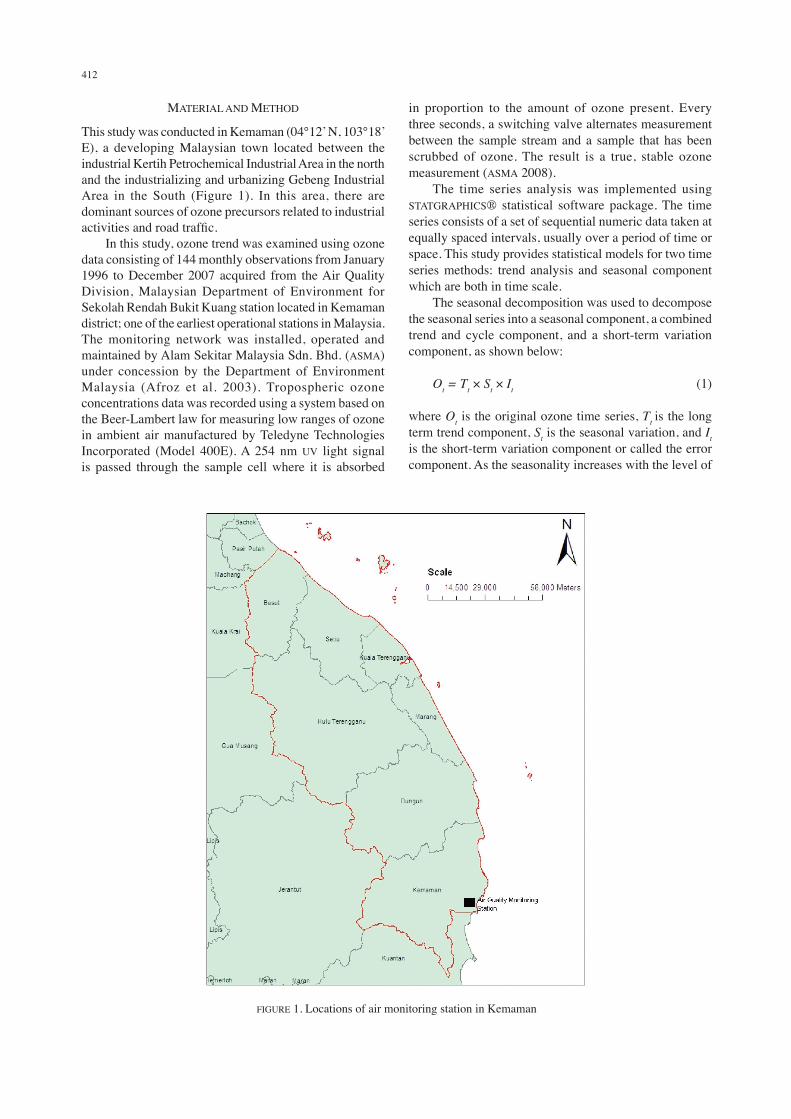
This study was conducted in Kemaman (04°12’ N, 103°18’ E), a developing Malaysian town located between the industrial Kertih Petrochemical Industrial Area in the north and the industrializing and urbanizing Gebeng Industrial Area in the South (Figure 1). In this area, there are dominant sources of ozone precursors related to industrial activities and road traffic. In this study, ozone trend was examined using ozone data consisting of 144 monthly observations from January 1996 to December 2007 acquired from the Air Quality Division, Malaysian Department of Environment for Sekolah Rendah Bukit Kuang station located in Kemaman district; one of the earliest operational stations in Malaysia. The monitoring network was installed, operated and maintained by Alam Sekitar Malaysia Sdn. Bhd. (ASMA) under concession by the Department of Environment Malaysia (Afroz et al. 2003). Tropospheric ozone concentrations data was recorded using a system based on the Beer-Lambert law for measuring low ranges of ozone in ambient air manufactured by Teledyne Technologies Incorporated (Model 400E). A 254 nm UV light signal is passed through the sample cell where it is absorbed

in proportion to the amount of ozone present. Every three seconds, a switching valve alternates measurement between the sample stream and a sample that has been scrubbed of ozone. The result is a true, stable ozone measurement (ASMA 2008). The time series analysis was implemented using STATGRAPHICS® statistical software package. The time series consists of a set of sequential numeric data taken at equally spaced intervals, usually over a period of time or space. This study provides statistical models for two time series methods: trend analysis and seasonal component which are both in time scale. The seasonal decomposition was used to decompose the seasonal series into a seasonal component, a combined trend and cycle component, and a short-term variation component, as shown below:

Ot = Tt × St × It (1)

where Ot is the original ozone time series, Tt is the long term trend component, St is the seasonal variation, and It is the short-term variation component or called the error component. As the seasonality increases with the level of

FIGURE 1. Locations of air monitoring station in Kemaman

413

the series, a multiplicative model was used to estimate the seasonal index. Under this model, the trend has the same units as the original series, but the seasonal and irregular components are unitless factors, distributed around 1. As the underlying level of the series changes, the magnitude of the seasonal fluctuations varies as well. The seasonal index was the average deviation of each month’s ozone value from the ozone level that was due to the other components in that month. In trend analysis, Box-Jenkins Autoregressive Integrated Moving Average (ARIMA) model was applied to model the time series behavior in generating the forecasting trend. The method which consists of a four-step iterative procedure was used in this study. The first step is model identification, where the historical data are used to tentatively identify an appropriate Box-Jenkins model followed by estimation of the parameters of the tentatively identified model. Subsequently, the diagnostic checking step must be executed to check the adequacy of the identified model in order to choose the best model. A better model ought to be identified if the model is inadequate. Finally, the best model is used to establish the time series forecasting value. In model identification (step 1), the data were examined to check for the most appropriate class of ARIMA processes through selecting the order of the consecutive and seasonal differencing required to make the series stationary, as well as specifying the order of the regular and seasonal auto regressive and moving average polynomials necessary to adequately represent the time series model. The Autocorrelation Function (ACF) and the Partial Autocorrelation Function (PACF) are the most important elements of the time series analysis and forecasting. The ACF measures the amount of linear dependence between observations in a time series that are separated by a lag k. The PACF plot helps to determine how many auto regressive terms are necessary to reveal one or more of the following characteristics: time lags where high correlations appear, seasonality of the series, trend either in the mean level or in the variance of the series. The general model introduced by Box and Jenkins includes autoregressive and moving average parameters as well as differencing in the formulation of the model. The three types of parameters in the model are the autoregressive parameters (p), the number of differencing passes (d) and moving average parameters (q). Box-Jenkins model are summarized as ARIMA (p, d, q). For example, a model described as ARIMA (1,1,1) means that this contains 1 autoregressive (p) parameter and 1 moving average (q) parameter for the time series data after it was differenced once to attain stationary. In addition to the non-seasonal ARIMA (p, d, q) model introduced above, we could identify seasonal ARIMA (P, D, Q) parameters for our data. These parameters are seasonal autoregressive (P), seasonal differencing (D) and seasonal moving average (Q). Seasonality is defined as a pattern that repeats itself over fixed interval of time. In general, seasonality can be

found by identifying a large autocorrelation coefficient or large partial autocorrelation coefficient at a seasonal lag. For example, ARIMA (1,1,1)(1,1,1)12 describes a model that includes 1 autoregressive parameter, 1 moving average parameter, 1 seasonal autoregressive parameter and 1 seasonal moving average parameter. These parameters were computed after the series was differenced once at lag 1 and differenced once at lag 12. The general form of the above model describing the current value Zt of a time series by its own past is shown in (2):

(1-φ1B)(1-α1 B12)(1-B)(1-B12) Zt= (1-θ1B) (1-γ1B

12) et

(2)

where 1-φ1B is the non seasonal autoregressive of order 1, 1-α1 B

12 is the seasonal autoregressive of order 1, Zt is the current value of the time series examined, B is the backward shift operator BZt = Zt-1 and B12Zt= Zt-12, 1-B is the 1st order non-seasonal difference, 1-B12 is the seasonal difference of order 1, 1-θ1B is the non seasonal moving average of order 1 and 1-γ1B

12 is the seasonal moving average of order 1. For the seasonal model, we used the Akaike Information Criterion (AIC) for model selection. The AIC is a combination of two conflicting factors: the mean square error and the number of estimated parameters of a model. Generally the model with smallest value of AIC is chosen as the best model (Hong 1997). After choosing the most appropriate model, the model parameters are estimated (step 2) - the plot of the ACF and PACF of the stationary data was examined to identify what autoregressive or moving average terms are suggested. Here, the values of the parameters are chosen using the least square method to make the Sum of the Squared Residuals (SSR) between the real data and the estimated values as small as possible. In most cases, nonlinear estimation method is used to estimate the above identified parameters to maximize the likelihood (probability) of the observed series given the parameter values (Naill & Momani 2009). In diagnose checking step (step 3), the residuals from the fitted model is examined against adequacy. This is usually done by correlation analysis through the residual ACF plots and the goodness-of-fit test by means of Chi-square statistics χ2. If the residuals are correlated, then the model should be refined as in step one above. Otherwise, the autocorrelations are white noise and the model is adequate to represent our time series. The final stage for the modeling process (step 4) is forecasting, which gives results as three different options: forecasted values, upper and lower limits that provide a confidence interval of 95%. Any forecasted values within the confidence limit are satisfactory. Finally, the accuracy of the model is checked with the Mean-Square error (MS) to compare fits of different ARIMA models. A lower MS value corresponds to a better fitting model.

414

RESULTS AND DISCUSSION

The first step in time series analysis is to draw time series plot which provides a preliminary understanding of time behavior of the series as shown in Figure 2. Trend of the original series appear to be slightly increasing. Nonetheless, this needs to be tested and confirmed through descriptive analysis and trend modeling. In seasonality of ozone, a well-defined annual cycle was consistent with the highest ozone means occurring in August, and the lowest ozone means in November as shown in Figure 3. Table 1 illustrates the seasonal indices range from a low of 80.047 in November to a high of 122.058 in August. This indicates that there is a seasonal swing from 80.047% of average to 122.058% of average throughout the course of one complete cycle i.e. one year. The seasonal variation pattern in Kemaman differed from other countries, such as United States, United Kingdom, Italy, Canada, and Japan, in that the peak ozone concentration did not correspond to maximum photochemical activity in summer (Angle & Sandhu 1989; Colbeck & MacKenzie 1994; Lorenzini et al. 1994).

For the purpose of forecasting the trend in this study, the first 132 observations (January 1996 to December 2006) were used to fit the ARIMA models while the subsequent 12 observations (from January 2007 to December 2007) were kept for the post sample forecast accuracy check. Ozone concentrations data has been adjusted in the following way before the model was fitted simple differences of order 1 and seasonal differences of order 1 were taken. The model with the lowest value (-11.8601) of the Akaike Information Criterion (AIC) as shown in Table 3 is (ARIMA) (0, 1, 1) × (1, 1, 2)12; was selected and has been used to generate the forecasts (Figure 4). This model assumes that the best forecast for future data is given by a parametric model relating the most recent data value to previous data values and previous noise. As shown in Table 2, the P-value for the MA (1) term, SAR (1) term, SMA (1) term and SMA (2) term, respectively are less than 0.05, so they are significantly different from 0. Meanwhile, the estimated standard deviation of the input white noise equals 0.00277984. Since no tests are statistically significant at the 95% or higher confidence level, the current model is adequate to represent the data and could be used to forecast the

Year

O3(p

pm)

FIGURE 2. Original monthly ozone concentration for Kemaman

Month

Seas

onal

inde

x

FIGURE 3. Annual variation of monthly ozone means (1996-2007)

415

upcoming ozone concentration. Therefore, we can assume that the best model for ground level ozone in Kemaman is the mathematical expression as shown below:

Z(t) = a(t) + 0.53a(t – 12) – 0.82(t – 1) – 1.67a(t – 12) + 0.73a(t – 2) + 0.82(1.67)a(t – 13) – 0.82(0.73) a(t – 25).

(3)

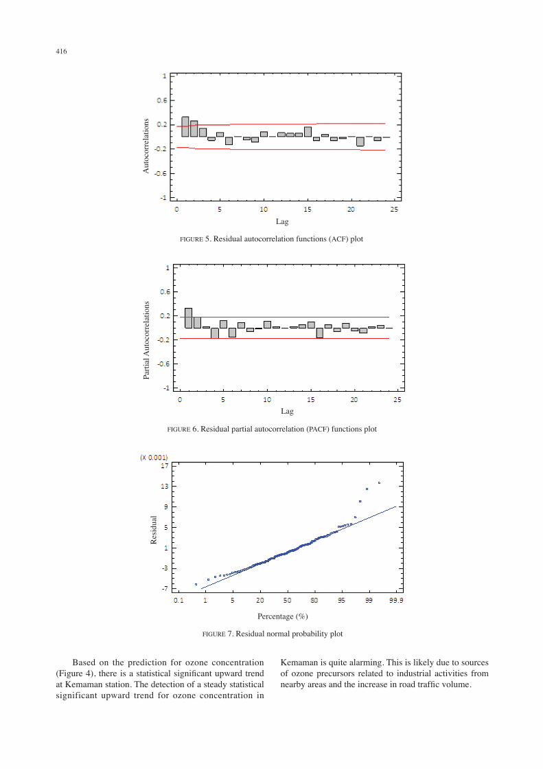
According to plots of residual ACF (Figure 5) and PACF (Figure 6), residuals are white noise and not-auto correlated. Furthermore, as shown in Figure 7 of normal probability plot, residuals of the model are normal.

TABLE 1. Seasonal index of ozone (1996-2007)

Month Seasonal indexJanuaryFebruaryMarchAprilMayJuneJulyAugustSeptemberOctoberNovemberDecember

107.19990.825984.717980.7204101.135105.618115.073122.058117.77193.094180.0473101.741

TABLE 2. ARIMA (0, 1, 1) × (1, 1, 2)12 model parameter characteristics

Parameter Estimate Stnd. Error T P-value

MA(1)SAR(1)SMA(1)SMA(2)

0.8187860.5317451.67374-0.728689

0.04781330.1462130.0924740.081741

17.12463.6367818.0996-8.91461

0.0000000.0004000.0000000.000000

TABLE 3. Model comparison

Model* RMSE MAE MAPE ME MPE AIC

(A)(B)(C)(H)(I)(J)(M)(N)(O)(P)(Q)

0.003370.002710.002690.002670.002710.002700.002580.002570.002580.002590.00259

0.002490.002060.002010.001980.002010.001990.002060.002040.002060.002070.00207

13.52611.08610.78610.70710.87010.67111.25011.19211.29811.26011.267

0.0000040.0000020.0000020.000003-0.0000500.0002060.000031-0.00009-0.000053

0.000030

-1.5017-1.8498-1.8157-1.7185-1.9817-0.5469-1.5638-2.0636-1.9673-1.7473-1.5789

-11.2253-11.6431-11.6409-11.6712-11.6423-11.6286-11.8601-11.8478-11.8392-11.8382-11.8335

*Models (A) Random walk; (B) Constant mean = 0.0190056; (C) Linear trend = 0.0184806 + 0.00000789502 t (H) Simple exponential smoothing with = 0.109; (I) Brown's linear exp. smoothing with α = 0.0572(J) Holt's linear exp. smoothing with α = 0.1291 and β = 0.0301; (M) ARIMA(0,1,1)×(1,1,2)12 (N) ARIMA(1,0,1)×(1,1,2)12; (O) ARIMA(0,1,1)×(1,1,2)12 with constant (P) ARIMA(0,1,1)×(2,1,2)12; (Q) ARIMA(0,1,2)x(1,1,2)12

Year

Ozo

ne (p

pm)

FIGURE 4. Model predicted plot of ozone concentration with actual and 95% confidence band

actualforecast95.0% limits

416

Based on the prediction for ozone concentration (Figure 4), there is a statistical significant upward trend at Kemaman station. The detection of a steady statistical significant upward trend for ozone concentration in

Kemaman is quite alarming. This is likely due to sources of ozone precursors related to industrial activities from nearby areas and the increase in road traffic volume.

Aut

ocor

rela

tions

Lag

FIGURE 5. Residual autocorrelation functions (ACF) plot

Parti

al A

utoc

orre

latio

ns

Lag

FIGURE 6. Residual partial autocorrelation (PACF) functions plot

Res

idua

l

Percentage (%)

FIGURE 7. Residual normal probability plot

417

CONCLUSIONS

Time series analysis is an important tool in modeling and forecasting air pollutants. Although, this information is not appropriate to predict the exact monthly ozone concentration, ARIMA (0, 1, 1) × (1, 1, 2)12 model give us information that can help the decision makers to establish strategies, priorities and proper use of fossil fuel resources in Kemaman. This is very important because ground level ozone (O3) is formed from NOx and VOCs brought about by human activities (largely the combustion of fossil fuel). Compliance with the Malaysian air pollution guideline for ozone was achieved because the ozone concentrations averaged over any 8 hours did not exceed 60 ppb but many studies throughout Europe and in the United States has practically determined 40 ppb as the threshold value, below which the losses of crops due to ozone exposure could be neglected, and above which the losses are assumed to be linear with respect to the exposure (Gerosa et al. 2007; Mills et al. 2007). In summary, the ozone level increased steadily in Kemaman area and is predicted to exceed 40 ppb by 2019 if no effective countermeasures are introduced.

ACKNOWLEDGEMENTS

The authors thank DOE Malaysia for providing pollutants data from 1996-2007 and the Ministry of Higher Education (MOHE) for allocating the research grant to conduct this study.

REFERENCES

Afroz, R., Hassan, M.N. & Ibrahim, N.A. 2003. Review of air pollution and health impacts in Malaysia. Journal of Environmental Research 92(2): 71-77.

Angle, R.P. & Sandhu, H.S. 1989. Urban and Rural Ozone Concentrations in Alberta, Canada. Atmospheric Environment 23: 215- 221.

Bencala, K.E. & Seinfield, J.H. 1979. On Frequency distribution of air pollutant concentrations. Atmospheric Environment 10: 941-950.

Chan, C.Y. & Chan, L.Y. 2000. The effect of meteorology and air pollutant transport on ozone episodes at a subtropical coastal asian city, Hong Kong. Journal of Geophysical Research 105: 20707-20719.

Colbeck, I. & MacKenzie, A.R. 1994. Air Quality Monographs, Air Pollution by Photochemical Oxidants. Vol.1. Amsterdam: Elsevier, pp. 107-71.

Gerosa G., Ferretti M., Bussotti F. & Rocchini D. 2007. Estimates of ozone AOT40 from passive sampling in forest sites in South-Western Europe. Environmental Pollution 145(3): 629-635

Gouveia, N. & Fletcher, T. 2000. Time series analysis of air pollution and mortality: Effects by cause, age and socioeconomic status. Journal of Epidemiology and Community Health 54: 750-755.

Hertzberg, A.M. & Frew, L. 2003. Can public policy be influenced? Environmetrics 14(1): 1-10.

Hies, T., Treffeisen, R., Sebald, L. & Reimer, E. 2003. Spectral analysis of air pollutants. Part I: Elemental carbon time series. Atmospheric Environment 34: 3495-3502.

Hong, W. 1997. A Time Series Analysis of United States Carrots Exports to Canada. MSc Thesis, North Dakota State University.

Kocak, K., Saylan, L. & Sen, O. 2000. Nonlinear time series prediction of O3 concentration in Istanbul. Atmospheric Environment 34: 1267-1271.

Kyriakidis, P.C. & Journal, A.G. 2001. Stochastic modelling of atmospheric pollution: A special time series framework, part II: Application to monitoring monthly sulfate deposition over Europe. Atmospheric Environment 35: 2339-2348.

Lee, C.K. 2002. Multiracial Characteristics in air pollutant concentration time series. Journal of Water, Air & Soil Pollution 135: 389-409.

Liu, C.M., Hung, C.Y., Shieh, S.L. & Wu, C.C. 1994. Important meteorological parameters for ozone episodes experienced in the Taipei basin. Atmospheric Environment 28: 159-173.

Lorenzini, G., Nali, C. & Panicucci, A. 1994. Surface ozone in Pisa (Italy): A six year study. Atmospheric Environment 28: 3155-3164.

Mills, G., Buse, A., Gimeno, B., Bermejo, V., Holland, M., Emberson, L. & Pleijel, H. 2007. A synthesis of AOT40-based response functions and critical levels of ozone for agricultural and horticultural crops. Atmospheric Environment 41: 2630-2643

Naill, P.E. & Momani, M. 2009. Time series analysis model for rainfall data in Jordan: Case study for using time series analysis. American Journal of Environmental Sciences 5(5): 599-604.

Roberts, S. 2003. Combining data from multiple monitors in air pollution mortality time series studies. Atmospheric Environment 35: 2339-2348.

Salcedo, R.L.R., Alvim, F.M., Alves, C. & Martins, F. 1999. Time series analysis of air pollution data. Atmospheric Environment 33: 2361-2372.

Schwartz, J. & Marcus, A. 1990. Mortality and air pollution in London: A time series analysis. American Journal of Epidemiology 131: 85-194.

Touloumi, G., Atkinson, R. & Terte, A.L. 2004. Analysis of health outcome time series data in epidemiological studies. Environmetrics 15: 101-117.

Wu, H.W.Y. & Chan, L.Y. 2001. Surface ozone trends in Hong Kong in 1985-1995. Journal of Environmental International 26: 213-222.

Yee, E. & Chen, R. 1997. A simple model for probability density functions of concentration fluctuations in atmospheric plumes. Atmospheric Environment 31: 991-1002.

Marzuki Ismail*, Mohd Zamri Ibrahim & Tg. Azmina IbrahimDepartment of Engineering ScienceFaculty of Science and TechnologyUniversiti Malaysia Terengganu21030 Kuala TerengganuTerengganu, Malaysia

Ahmad Makmon AbdullahDepartment of Environmental ScienceFaulty of Environmental StudiesUniversiti Putra Malaysia43300 SerdangSelangor, Malaysia

*Corresponding author; email: marzuki@umt.edu.my

Received: 30 March 2010Accepted: 29 September 2010