VOT 78138

UNCERTAINTY OF PHOSPHORUS LOADINGS ESTIMATION USING

VOLLENWEIDER MODEL FOR RESERVOIR EUTROPHICATION

CONTROL

(KETAKPASTIAN BEBANAN FOSFORUS MENGGUNAKAN MODEL

VOLLENWEIDER UNTUK KAWALAN EUTROFIKASI TAKUNGAN)

SUPIAH SHAMSUDIN SOBRI HARUN

AZMI AB RAHMAN

PUSAT PENGURUSAN PENYELIDIKAN UNIVERSITI TEKNOLOGI MALAYSIA

2009

UNCERTAINTY OF PHOSPHORUS LOADINGS ESTIMATION USING

VOLLENWEIDER MODEL FOR RESERVOIR EUTROPHICATION

CONTROL

(KETAKPASTIAN BEBANAN FOSFORUS MENGGUNAKAN MODEL

VOLLENWEIDER UNTUK KAWALAN EUTROFIKASI TAKUNGAN)

SUPIAH SHAMSUDIN SOBRI HARUN

AZMI AB RAHMAN

RESEARCH VOTE NO:

78138

Jabatan Hidraul dan Hidrologi

Fakulti Kejuruteraan Awam Universiti Teknologi Malaysia

2009

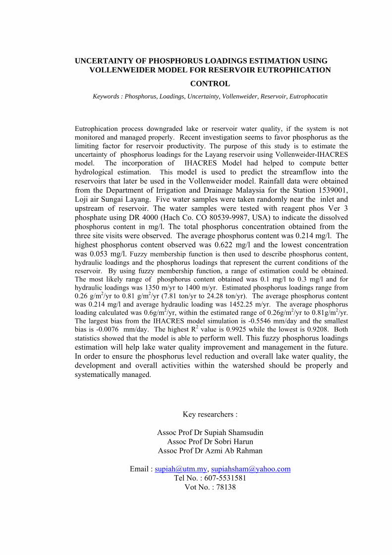
UNCERTAINTY OF PHOSPHORUS LOADINGS ESTIMATION USING VOLLENWEIDER MODEL FOR RESERVOIR EUTROPHICATION

CONTROL Keywords : Phosphorus, Loadings, Uncertainty, Vollenweider, Reservoir, Eutrophocatin

Eutrophication process downgraded lake or reservoir water quality, if the system is not monitored and managed properly. Recent investigation seems to favor phosphorus as the limiting factor for reservoir productivity. The purpose of this study is to estimate the uncertainty of phosphorus loadings for the Layang reservoir using Vollenweider-IHACRES model. The incorporation of IHACRES Model had helped to compute better hydrological estimation. This model is used to predict the streamflow into the reservoirs that later be used in the Vollenweider model. Rainfall data were obtained from the Department of Irrigation and Drainage Malaysia for the Station 1539001, Loji air Sungai Layang. Five water samples were taken randomly near the inlet and upstream of reservoir. The water samples were tested with reagent phos Ver 3 phosphate using DR 4000 (Hach Co. CO 80539-9987, USA) to indicate the dissolved phosphorus content in mg/l. The total phosphorus concentration obtained from the three site visits were observed. The average phosphorus content was 0.214 mg/l. The highest phosphorus content observed was 0.622 mg/l and the lowest concentration was 0.053 mg/l. Fuzzy membership function is then used to describe phosphorus content, hydraulic loadings and the phosphorus loadings that represent the current conditions of the reservoir. By using fuzzy membership function, a range of estimation could be obtained. The most likely range of phosphorus content obtained was 0.1 mg/l to 0.3 mg/l and for hydraulic loadings was 1350 m/yr to 1400 m/yr. Estimated phosphorus loadings range from 0.26 g/m2/yr to 0.81 g/m2/yr (7.81 ton/yr to 24.28 ton/yr). The average phosphorus content was 0.214 mg/l and average hydraulic loading was 1452.25 m/yr. The average phosphorus loading calculated was 0.6g/m2/yr, within the estimated range of 0.26g/m2/yr to 0.81g/m2/yr. The largest bias from the IHACRES model simulation is -0.5546 mm/day and the smallest bias is -0.0076 mm/day. The highest R2 value is 0.9925 while the lowest is 0.9208. Both statistics showed that the model is able to perform well. This fuzzy phosphorus loadings estimation will help lake water quality improvement and management in the future. In order to ensure the phosphorus level reduction and overall lake water quality, the development and overall activities within the watershed should be properly and systematically managed.

Key researchers :

Assoc Prof Dr Supiah Shamsudin Assoc Prof Dr Sobri Harun

Assoc Prof Dr Azmi Ab Rahman

Email : supiah@utm.my, supiahsham@yahoo.com Tel No. : 607-5531581

Vot No. : 78138

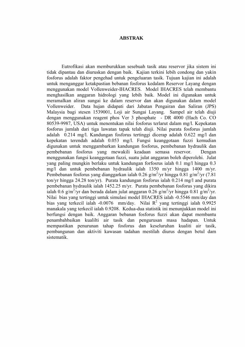
ABSTRAK Eutrofikasi akan memburukkan sesebuah tasik atau reservor jika sistem ini tidak dipantau dan diuruskan dengan baik. Kajian terkini lebih condong dan yakin fosforus adalah faktor pengehad untuk pengeluaran tasik. Tujuan kajian ini adalah untuk menganggar ketakpastian bebanan fosforus kedalam Reservor Layang dengan menggunakan model Vollenweider-IHACRES. Model IHACRES telah membantu menghasilkan anggaran hidrologi yang lebih baik. Model ini digunakan untuk meramalkan aliran sungai ke dalam reservor dan akan digunakan dalam model Vollenweider. Data hujan didapati dari Jabatan Pengairan dan Saliran (JPS) Malaysia bagi stesen 1539001, Loji air Sungai Layang. Sampel air telah diuji dengan menggunakan reagent phos Ver 3 phosphate - DR 4000 (Hach Co. CO 80539-9987, USA) untuk menentukan nilai fosforus terlarut dalam mg/l. Kepekatan fosforus jumlah dari tiga lawatan tapak telah diuji. Nilai purata fosforus jumlah adalah 0.214 mg/l. Kandungan fosforus tertinggi dicerap adalah 0.622 mg/l dan kepekatan terendah adalah 0.053 mg/l. Fungsi keanggotaan fuzzi kemudian digunakan untuk menggambarkan kandungan fosforus, pembebanan hydraulik dan pembebanan fosforus yang mewakili keadaan semasa reservor. Dengan menggunakan fungsi keanggotaan fuzzi, suatu julat anggaran boleh diperolehi. Julat yang paling mungkin berlaku untuk kandungan forfosrus ialah 0.1 mg/l hingga 0.3 mg/l dan untuk pembebanan hydraulik ialah 1350 m/yr hingga 1400 m/yr. Pembebanan fosforus yang dianggarkan ialah 0.26 g/m2/yr hingga 0.81 g/m2/yr (7.81 ton/yr hingga 24.28 ton/yr). Purata kandungan fosforus ialah 0.214 mg/l and purata pembebanan hydraulik ialah 1452.25 m/yr. Purata pembebanan fosforus yang dikira ialah 0.6 g/m2/yr dan berada dalam julat anggaran 0.26 g/m2/yr hingga 0.81 g/m2/yr. Nilai bias yang tertinggi untuk simulasi model IHACRES ialah -0.5546 mm/day dan bias yang terkecil ialah -0.0076 mm/day. Nilai R2 yang tertinggi ialah 0.9925 manakala yang terkecil ialah 0.9208. Kedua-dua statistik ini menunjukkan model ini berfungsi dengan baik. Anggaran bebanan fosforus fuzzi akan dapat membantu penambahbaikan kualilti air tasik dan pengurusan masa hadapan. Untuk mempastikan penurunan tahap fosforus dan keseluruhan kualiti air tasik, pembangunan dan aktiviti kawasan tadahan mestilah diurus dengan betul dam sistematik.

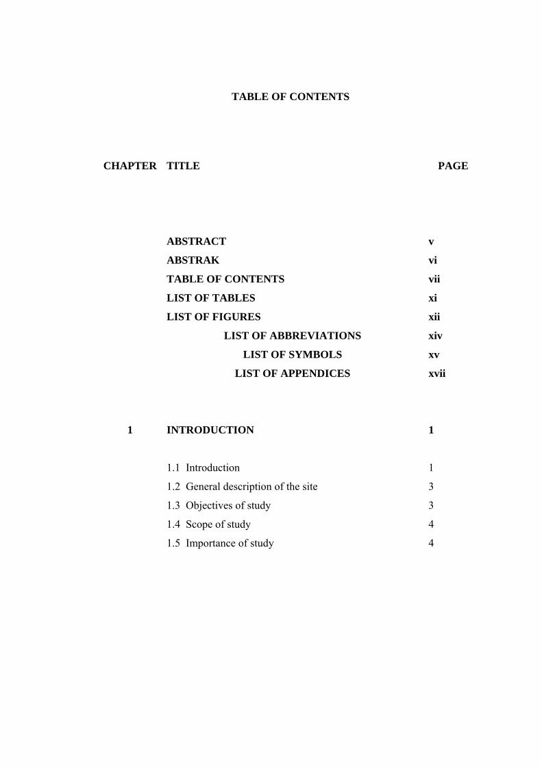
TABLE OF CONTENTS

CHAPTER TITLE PAGE

ABSTRACT v

ABSTRAK vi

TABLE OF CONTENTS vii

LIST OF TABLES xi

LIST OF FIGURES xii

LIST OF ABBREVIATIONS xiv

LIST OF SYMBOLS xv

LIST OF APPENDICES xvii

1 INTRODUCTION

1.1 Introduction

1.2 General description of the site

1.3 Objectives of study

1.4 Scope of study

1.5 Importance of study

1

1

3

3

4

4

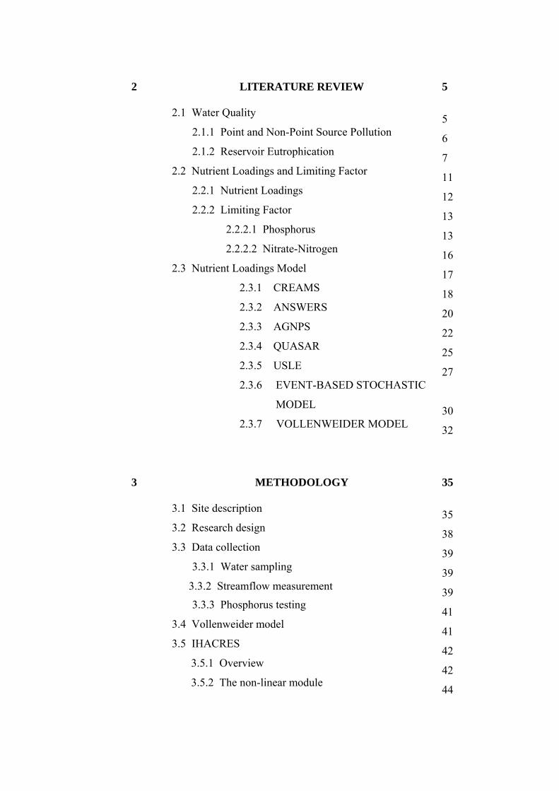
2 LITERATURE REVIEW 2.1 Water Quality

2.1.1 Point and Non-Point Source Pollution

2.1.2 Reservoir Eutrophication

2.2 Nutrient Loadings and Limiting Factor

2.2.1 Nutrient Loadings

2.2.2 Limiting Factor

2.2.2.1 Phosphorus

2.2.2.2 Nitrate-Nitrogen

2.3 Nutrient Loadings Model

2.3.1 CREAMS

2.3.2 ANSWERS

2.3.3 AGNPS

2.3.4 QUASAR

2.3.5 USLE

2.3.6 EVENT-BASED STOCHASTIC

MODEL

2.3.7 VOLLENWEIDER MODEL

5

5

6

7

11

12

13

13

16

17

18

20

22

25

27

30

32

3 METHODOLOGY 3.1 Site description

3.2 Research design

3.3 Data collection

3.3.1 Water sampling

3.3.2 Streamflow measurement

3.3.3 Phosphorus testing

3.4 Vollenweider model

3.5 IHACRES

3.5.1 Overview

3.5.2 The non-linear module

35

35

38

39

39

39

41

41

42

42

44

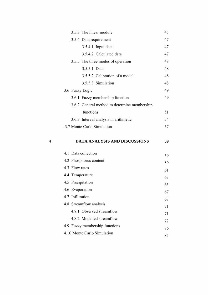
3.5.3 The linear module

3.5.4 Data requirement

3.5.4.1 Input data

3.5.4.2 Calculated data

3.5.5 The three modes of operation

3.5.5.1 Data

3.5.5.2 Calibration of a model

3.5.5.3 Simulation

3.6 Fuzzy Logic

3.6.1 Fuzzy membership function

3.6.2 General method to determine membership

functions

3.6.3 Interval analysis in arithmetic

3.7 Monte Carlo Simulation

45

47

47

47

48

48

48

48

49

49

51

54

57

4 DATA ANALYSIS AND DISCUSSIONS

4.1 Data collection

4.2 Phosphorus content

4.3 Flow rates

4.4 Temperature

4.5 Precipitation

4.6 Evaporation

4.7 Infiltration

4.8 Streamflow analysis

4.8.1 Observed streamflow

4.8.2 Modelled streamflow

4.9 Fuzzy membership functions

4.10 Monte Carlo Simulation

59

59

59

61

63

65

67

67

71

71

72

76

85

5 CONCLUSIONS AND RECOMMENDATIONS

5.1 Conclusions

5.2 Recommendations

88

88

89

REFERENCES

90

APPENDICES

93-98

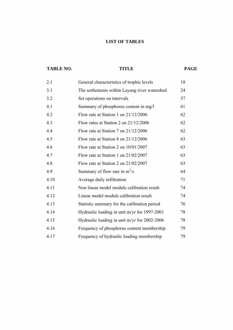
LIST OF TABLES

TABLE NO. TITLE PAGE

2.1 General characteristics of trophic levels 18

3.1 The settlements within Layang river watershed 24

3.2 Set operations on intervals 57

4.1 Summary of phosphorus content in mg/l 61

4.2 Flow rate at Station 1 on 21/12/2006 62

4.3 Flow rates at Station 2 on 21/12/2006 62

4.4 Flow rate at Station 7 on 21/12/2006 62

4.5 Flow rate at Station 8 on 21/12/2006 63

4.6 Flow rate at Station 2 on 10/01/2007 63

4.7 Flow rate at Station 1 on 21/02/2007 63

4.8 Flow rate at Station 2 on 21/02/2007 63

4.9 Summary of flow rate in m3/s 64

4.10 Average daily infiltration 71

4.11 Non linear model module calibration result 74

4.12 Linear model module calibration result 74

4.13 Statistic summary for the calibration period 76

4.14 Hydraulic loading in unit m/yr for 1997-2001 78

4.15 Hydraulic loading in unit m/yr for 2002-2006 78

4.16 Frequency of phosphorus content membership 79

4.17 Frequency of hydraulic loading membership 79

LIST OF FIGURES

FIGURE NO. TITLE PAGE

2.1 The hydrologic cycle 6

2.2 The zones of a lake 11

2.3 The basic phosphorus cycle in an aquatic system 20

2.4 The graph of algal biomass vs total phosphorus 21

3.1 Location of Layang reservoir 25

3.2 Flow chart of methodology 26

3.3 Mid section method 28

3.4 The system structure of the rainfall - runoff model 31

3.5 Unit effective rainfall 33

3.6 Resultant unit hydrograph 33

3.7 Data > Summary screen 37

3.8 Data > Import screen 37

3.9 Synchronisation Summary message box 39

3.10 Data > View screen 40

3.11 Calibration > Model screen 41

3.12 Calibration > Periods screen 42

3.13 Grid search parameters 44

3.14 Grid search results 45

3.15 Analysis for most effective grid search result 46

3.16 Accepted parameter sets message box 47

3.17 Calibration > Model screen after the model is

calibrated

48

3.18 Hydrograph of modelled vs observed streamflow 49

3.19 Simulation Summary screen 50

3.20 Statistic Summary for the simulated results 50

3.21 Multiple options for creating charts 51

3.22 The features in a fuzzy membership function 53

3.23 A random experiment (A is fixed but ω varies) 55

3.24 A fuzzy statistical experiment ( is fixed but A0u *

varies)

56

4.1 Total phosphorus concentration from the three site

visits

61

4.2 Flow rates from the three site visits 64

4.3 Graph of temperature 65

4.4 Daily rainfall of Layang (Station 1539001) 67

4.5 Daily evaporation of Layang (Station 1539301) 69

4.6 Average daily infiltration 71

4.7 Graph of modelled streamflow vs observed

streamflow

75

4.8 Average daily bias for the simulation period 76

4.9 R squared value for the simulation period 77

4.10 Histogram and membership function for

phosphorus content

81

4.11 Histogram and membership function for hydraulic

loading

81

4.12 Membership function for phosphorus content 82

4.13 Membership function for hydraulic loading 82

4.14 Membership function for phosphorus loadings

in g/m2/yr

84

4.15 Membership function for phosphorus loadings

in ton/yr

85

LIST OF ABBREVIATIONS Co. - Company Eq. - Equation IHACRES - Identification of unit Hydrographs and Component flows

from Rainfalls, Evaporation and Streamflow data Inc. - Incorporated Ltd. - Limited MASMA - Manual Mesra Alam NA - Not available UH - Unit hydrograph Vol. - Volume

LIST OF SYMBOLS A - Area

A - Event

A* - Crisp set

B - Width of each segment

C - Mass balance term

CO2 - Carbon dioxide

E - Evaporation

F - Infiltration

fo - Initial infiltration rate

fc - Final infiltration rate

f - Temperature dependence of drying rate

I - Inflow rate

K - Coefficient

L - Distance of segment from the river side

Lp - Annual areal P loading

Lc - Critical annual phosphorus loading

NH3 - Nitrate

O - Outflow rate

O2 - Oxygen

P - Precipitation

P - Phosphorus concentration in water

PO4 - Phosphate

Q - Discharge

Qo - Observed streamflow value

Qm - Modelled streamflow value

qs - Annual hydraulic loading

R - Reference temperature

R - Runoff

rk - Rainfall

sk - Streamflow

S - Condition

S - Storage

t - Time

tk - Temperature

T - Transpiration

Tw - Mean residence time of water in lake

uk - Effective rainfall

U. - Universe

uo - Fixed element

v - Velocity

y - Depth of river

z - Mean depth of lake

τw - Catchment drying rate at reference temperature

µ(x) - Elements x of the universe

Ω - Sample space

ω - Variable

LIST OF APPENDICES

APPENDIX TITLE PAGE

A Photos taken during site visit 91

B Tools and equipments used 95

CHAPTER 1

INTRODUCTION

1.1 Introduction

Water is a basic requirement for life on earth, including human life, crops,

livestock and fisheries for our food. Although 70% of the earth surface is covered by

water, which seems to be abundance, but not all the resources can be used. Only less

than 1% of the total amount is freshwater that is suitable for human use. Water is

used in many ways. Often, water is diverted from rivers, lakes, and aquifers to

supply domestic, livestock, agricultural irrigation, and various industrial uses (Wurbs

and James, 2002).

The management of water resources over a period of time will affect the

heath of the people, food security, prosperity of the country and even the future

survival. There has been an increase in the awareness related to issues regarding

water resources in Malaysia. As the country develops, more water supply is needed

for industrial, domestic, agriculture, and energy usages. Economic development is

also dependent on the water resources and water supply. Suitable water quality must

be reliably supplied for uses in individual homes, farms, and businesses.

Quality and quantity of water is related to each other. Over the years,

activities such as excessive development and urbanization, deforestation, and lack of

proper management of sewage treatment and discharge has lead to the increase in the

amount of pollution to the rivers. Polluted rivers will reduce the amount of clean

water available. If no proper way to overcome the problem, then the country may

face water crisis, such as water shortage in the future.

Eutrophication is another aspect regarding the pollution that will affect water

quality of the river if it is ignored for sometime. At first, eutrophication is a natural

process which will take a long time to happen, but then now the process is

accelerated by human activities, which include excessive usage of fertilizer in

agriculture, animal feeds, phosphorus components for detergents and other

commercial products which contains phosphorus element. Normally after use, most

of the phosphorus-contained wastes are just discharged into the environment. This

action will enhance the acceleration of the eutrophication rate of a water body such

as lake or reservoir (Schnoor, 1996).

Eutrophication is a process leading to over accelerated growth of the algae,

causing unpleasant odour, reducing the penetration of sun light, hence reduce the

dissolved oxygen inside the water, and this will further lead to the death of the living

organism inside the water. The dead organisms will contribute to the increment of

the sedimentation process at the waterbed. And finally the water will become

unsuitable for usage.

Clean and useable freshwater is a limited source and river is the main source

for water supply in Malaysia. The increasing needs of clean water supply plus the

shortage of available clean water supply at the same time will post a threat to the

community in the country.

1.2 General description of the site

Dams, reservoirs, and relating structures play a key role in water supply and

multi-purpose water management. Layang reservoir is selected for this study. This

reservoir serves as the water supply for the people around the area, which include

Johor Bahru (Sek, 1997).

The Layang reservoir is located near Masai, in Johor Bahru. The reservoir

can be divided into 2 parts, which are Hulu Layang reservoir and Hilir Layang

reservoir. The activities near the Layang river watershed mostly are villages,

plantation and agricultural estates. These areas are most likely to produce wastes and

effluents into the Layang river watershed. In other words, these are the sources of

potential pollution to the river.

1.3 Objectives of study

The research is done at the Layang catchment area which include the reservoir. The

objectives of this study are as follows :

1. To estimate the phosphorus loadings in the Layang reservoir using

Vollenweider model.

2. To predict the Layang river inflows into its reservoir using IHACRES model.

3. To incorporate fuzzy membership function in the estimation of phosphorus

loadings.

1.4 Scopes of study

1. Selected tools and equipments are used to obtain data for flow rates and water

samples at the site. Further testing is done at the laboratory on the water

samples with the use of suitable lab equipments to obtain the current

phosphorus content of the site area.

2. Simulation of IHACRES model is run to perceive the ability and performance

of the model in predicting the streamflow after acquiring all the relevent data.

3. The phosphorus loading of the reservoir can be estimated by using the

Vollenweider model after obtaining all the relevant and required data. Fuzzy

membership functions are used to describe the range of uncertainty for the

estimation of phosphorus loadings.

1.5 Importance of study

Malaysia is one of those fortunate countries in which water resources are

abundant. Under normal climatic trends, rain falls almost the entire year in all parts

of the country. Although the freshwater resources are renewable, they are also finite

and threatened by pollution from industrial, domestic, and agricultural wastes and

effluents. One of the consequences of these pollution is the effect on eutrophication.

The increase in the phosphorus load to water ecosystems can no longer be

compensated by the phosphorus holding capacity of lakes and reservoirs. It is a

necessity to manage the hydrological components of water storage, particularly lakes

and reservoirs for their optimal use while maintaining an ecological balance. This

study is to estimate the phosphorus loadings of the current state of the reservoir and

to explore new way of predicting streamflow of the river.

CHAPTER 2

LITERATURE REVIEW

The productivity of a reservoir is always measured by its water quality.

The water quality aspects focus on the water pollution problems and determine the

ability of a reservoir to perform its function foremost supplying good quality water

suitable enough for consumption. Pollutants from human activities have often caused

reservoirs to be contaminated. Point and non-point source pollution should be

controlled and regulated to improve the quality of the downstream water bodies

(Supiah, 2003). The need to understand the quality of reservoirs has long rises

attention to scientists and lake managers and to the publics as well. This chapter will

focuses on:

i) Water Quality

ii) Nutrient Loadings and Limiting Factor

iii) Nutrient Loading Model – Vollenweider Model

2.1 Water Quality

Originally, the intent of water quality management was to protect the

intended uses of a water body while using water as an economic means of waste

disposal within the constraints of its assimilative capacity (Davis and Masten, 2004).

Humans have depended on water so much that the environmental engineers must

properly design the treatment facilities to remove any pollutants to acceptable levels

without effecting the environment. Only by understanding how pollutants from

human activities affect water quality, the engineers is able to achieve this purpose

and come out with the solution.

2.1.1 Point and Non-Point Sources Pollution

The wide range of pollutants discharge to surface waters can be

grouped into two broad classes; point source and non-point source pollution. Point

source pollution comes from identified location where waste is discharged to the

receiving waters from a pipe or drain such as factories, sewage treatment plants, and

oil tankers. Most point source waste discharges are controlled by Department of

Environment (DOE) through a works approval and licensing system. The licence for

each input specifies the quality and quantity of the waste permitted to be discharged

to a river, lake or the sea at a particular location.

Pollution from non-point sources occurs when rainfall moves over and

through the ground. As the runoff moves, it picks up and carries away pollutants,

such as pesticides and fertilizers, depositing the pollutants into lakes, rivers,

wetlands, coastal waters, and even underground sources of drinking water. Pollution

arising from non-point sources accounts for a majority of the contaminants in

streams and lakes (Zimmerman, 2006). In a surface water body, non-point pollution

can contribute significantly to total pollutant loading, particularly with regard to

nutrients and pesticides.

Non-point pollution can have significant effects on wildlife and our

use of water (Vale, 2006). These effects include:

i) groundwater and surface water contamination

ii) microbiological contamination of water supplies

iii) nutrient enrichment and eutrophication

iv) oxygen depletion

v) toxicity to plant and animal life, including endocrine disruption in fish

2.1.2 Reservoir Eutrophication

Generally, the term “eutrophication” comes from the trophic state of lakes

where “eutrophic” means that lakes are high in nutrients supply in relation to volume

and dense growths of plankton in the surface waters. Lakes can be divided into three

categories based on trophic state; oligotrophic, mesotrophic, eutrophic and

hypereutrophic. These trophic descriptions are generally used to indicate the nutrient

status of a water body and describe the effects of nutrients on the general water

quality and clarity of a water body.

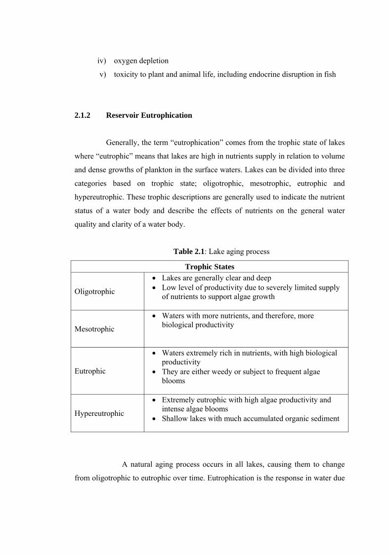
Table 2.1: Lake aging process

Trophic States

Oligotrophic

• Lakes are generally clear and deep • Low level of productivity due to severely limited supply

of nutrients to support algae growth

Mesotrophic

• Waters with more nutrients, and therefore, more biological productivity

Eutrophic

• Waters extremely rich in nutrients, with high biological productivity

• They are either weedy or subject to frequent algae blooms

Hypereutrophic

• Extremely eutrophic with high algae productivity and intense algae blooms

• Shallow lakes with much accumulated organic sediment

A natural aging process occurs in all lakes, causing them to change

from oligotrophic to eutrophic over time. Eutrophication is the response in water due

to over enrichment by nutrients, primarily phosphorus and nitrogen, and can occur

under natural or manmade conditions.

In the 1960s, eutrophication was recognized as a major water quality

problem affecting many valuable lakes, river, estuaries and coastal areas

(Vollenweider, 1987). There was much debate among scientist about the causes of

eutrophication. Some considered eutrophication a natural aging process, others

thought it involved climatic changes and some believed it was due to increasing

pollution. The latter cause was proven to be true and most scientists had agreed that

eutrophication was caused from excessive nutrients enrichment of lakes as a result of

human activity which has come to be known as “cultural eutrophication”.

Gilliom (1983) defined cultural eutrophication occurred due to the

high levels of nutrients that can quickly lead to undesirable growth of algae and other

aquatic plants, and to many related water quality problems. Davis and Masten (2004)

regarded cultural eutrophication of lakes can occur through the introduction of high

levels of nutrients, usually nitrogen and phosphorus, due to poor management of

watershed and the input of human and animal wastes. Human settlement in the

drainage basin of a lake generally leads to clearing of the natural vegetation, the

development of farms and cities. These activities accelerate runoff from the land

surface and increase the input of nutrient supply. Also, streams were convenient for

disposing of household wastes and sewage, adding to the nutrient load in the

receiving water body.

Cultural eutrophication is characterized by an intense proliferation of

algae and higher plants and their accumulation in excessive quantities, which can

result in detrimental changes in water quality and biological populations and can

interfere with human uses of that water body (Fisher et al., 1995). The term

eutrophication has been used increasingly to mean the artificial and undesirable

addition of plant nutrients, mainly P and N, to water bodies. The perceived negative

effects of cultural eutrophication include reduced water transparency and excessive

algal and plant growth, which is highly visible and can interfere with uses and

aesthetic quality of water. One consequence of such growths may be taste and odour

problems in drinking water. Ecological consequences include hypolimnetic anoxia

due to algal decomposition and fish kills and a rapid shift in species composition of

the biological community (Cooke et al., 2005). In tropical areas, diseases such as

malaria may be enhanced by eutrophication because the insect vector, mosquitoes in

the case of malaria, breeds in these waters. Other symptoms of cultural

eutrophication are:

i) Early stages symptoms consist of increase in phytoplankton standing

crop (biomass) and biomass at other trophic levels

ii) Algal blooms

iii) Complete depletion of oxygen from hypolimnion shortly after

stratification occurs: high concentrations of nutrients appear (due to

redox reactions)

iv) H2S, NH4+, non-mineralized organic matter, CH4 found in hypolimnion

as a result of anaerobic respiration

v) Invertebrate and fish communities change: species requiring high

oxygen levels disappear, species tolerant of low oxygen levels dominate.

Species diversity reduced.

2.1.2.1 Eutrophication Process

Traditionally, eutrophication referred only to nutrient loading, its eventual

high concentrations in the water column, and the high productivity and biomass of

algae that could occur. Organic matter loading may lead to sediment enrichment and

loss of volume. Organic matter, whether added to the water column from external or

internal sources, also leads to increased nutrient availability via direct mineralization,

or through release from sediments when respiration is stimulated by this organic

matter and DO is depleted.

Net internal P loading appears to increase exponentially with increasing

dissolved organic carbon content of the lake. Allochthonous organic matter contains

molecules producing changes in algal and microbial metabolism independently of

effects of added nutrients (Cooke et al., 2005). Finally, organic matter added to a

lake or reservoir contains energy that is incorporated, in both dissolved and

particulate forms, into plant and animal biomass, leading directly to increased living

biomass (the microbial loop). Dissolved and particulate organic matter entering the

lake or reservoir from streams, wetlands, and from macrophytes, is of great

significance to lake metabolism.

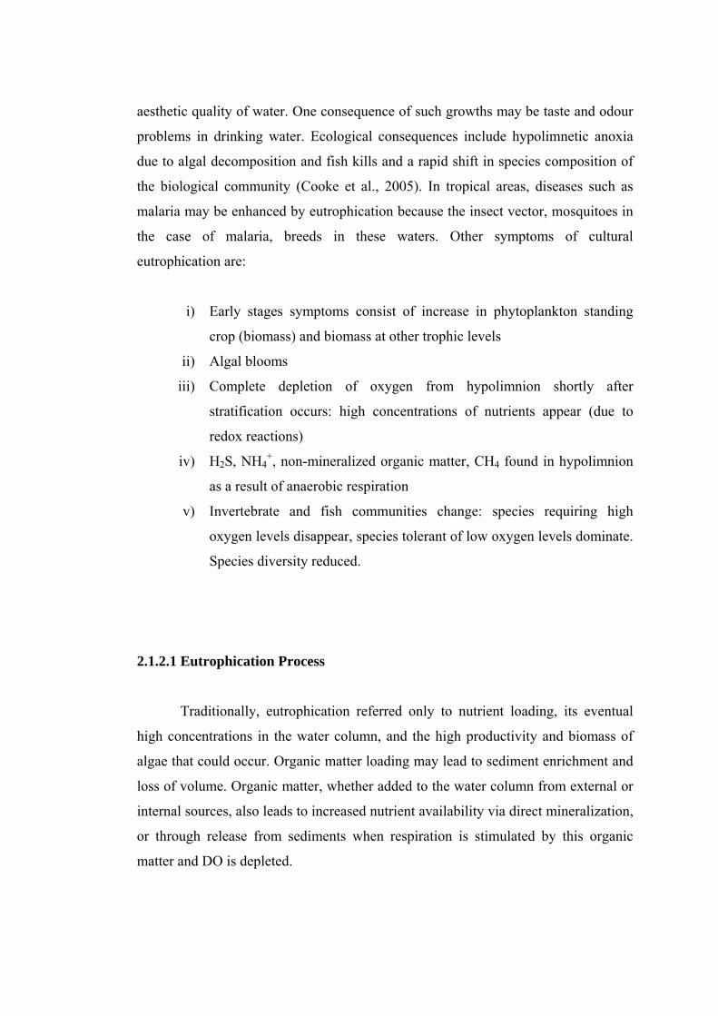
Silt may be rich in organic matter and in nutrients sorbed to surfaces of

particulate matter. These may become available to algae or macrophytes immediately

or at some later time. Silt loading also contributes directly to volume loss and to an

increase in shallow sediment area. Whether volume loss is produced by silt

deposition or by the build-up of refractory organic matter from terrestrial and aquatic

sources, the development of shallow areas fosters further spread of macrophytes and

their attendant epiphytic algae. Ultimately these plants promote further losses of DO

and release of organic molecules and nutrients as they decay (Figure 2.1).

Figure 2.1: Loadings and primary interactions in lakes and reservoirs

(Cooke et al., 2005)

Thus, silt and organic loadings have effects on lakes that are additional to

their nutrient content, and cannot be excluded when defining the eutrophication

process. This view is not meant to downplay or negate the fundamental importance

of high nutrient loading in stimulating lake productivity.

Excessive nutrient loading creates potential for eutrophic conditions but does

not guarantee increased productivity. Figure 2.1 does not account for the

“oligotrophication” effects of high rates of lake flushing and dilution, the effects of

organisms in stimulating nutrient release from sediments, or the effects of grazing (or

lack of grazing) on algae biomass. Lakes and reservoirs that are naturally eutrophic,

or have become so, have characteristics separating them from less enriched and

oligotrophic (“poorly nourished”) water bodies. Eutrophic lakes have algal “blooms,”

often of monospecific blue-green (cyanobacteria) populations. Some also have

macrophytes, though exotic macrophyte infestations are not a symptom of the

eutrophic condition because large populations can develop in oligotrophic waters.

Eutrophic lakes and reservoirs also have colored water (green or brown), and

low or zero DO levels in the deepest areas. Warm water fish production is likely to

be high. Fish can be limited by low DO and high pH, and lakes may be dominated by

less desirable fish species or stunted fish populations.

An oligotrophic lake or reservoir is low in nutrients and productivity because

organic matter and nutrient loadings are low or large basin water volumes and short

water residence times dilute or pass material through the lake. In addition, high water

hardness may foster co-precipitation of calcium carbonate and essential nutrients,

rendering them unavailable to algae. Oligotrophic lakes are often deep and steep-

sided, with nutrient-poor sediments, few macrophytes, usually no nuisance

cyanobacteria, and large amounts of DO in deep water. Water clarity is high, as is

phytoplankton diversity, but total algal biomass is low.

2.2 Nutrient Loadings and Limiting Factor

Alteration of the terrestrial landscape by man's activities has usually

enhanced the export of materials from the land to rivers and to the atmosphere

(Gilliom, 1983). As a result, many lakes, estuaries, and coastal waters experience

'cultural eutrophication' such as increased inflows of particulate and dissolved

materials, including N and P which promote the growth of algae if sufficient light is

available. Eutrophic aquatic systems often have large accumulations of algae and

sometimes macrophyte biomass, although N and P concentrations in the water may

be small if algae have assimilated and stored most of the incoming nutrients (Fisher

et al., 1995).

2.2.1 Nutrient Loadings

Nutrient loadings concept emerge from total conception that

eutrophication happened because of excessive amount of phosphorus (P) and

nitrogen (N). The water quality of lake is normally related to total nutrient loading.

Eutrophication of aquatic systems results from two sources of nutrient supply;

nutrient inputs from outside the aquatic system (external loading), and nutrient

recycling within the water column and sediments (internal loading). Natural and

anthropogenic processes influence both components of the nutrient supply.

External loading is usually enhanced by man through nutrient inputs

to streams and rivers from the fertilization of soils, soil erosion and disposal of

municipal or industrial effluents. Atmospheric deposition of both P and N may be

enhanced by anthropogenic emissions. The presence of large numbers of animals

may also disturb the watershed and increase the nutrient supply to aquatic systems.

F

column of nu

undisturbed la

is particularly

and ocean bas

greater distanc

relationship b

described in th

Inflow Loadin

2.2.2 Limiti

such as carbo

quantities) are

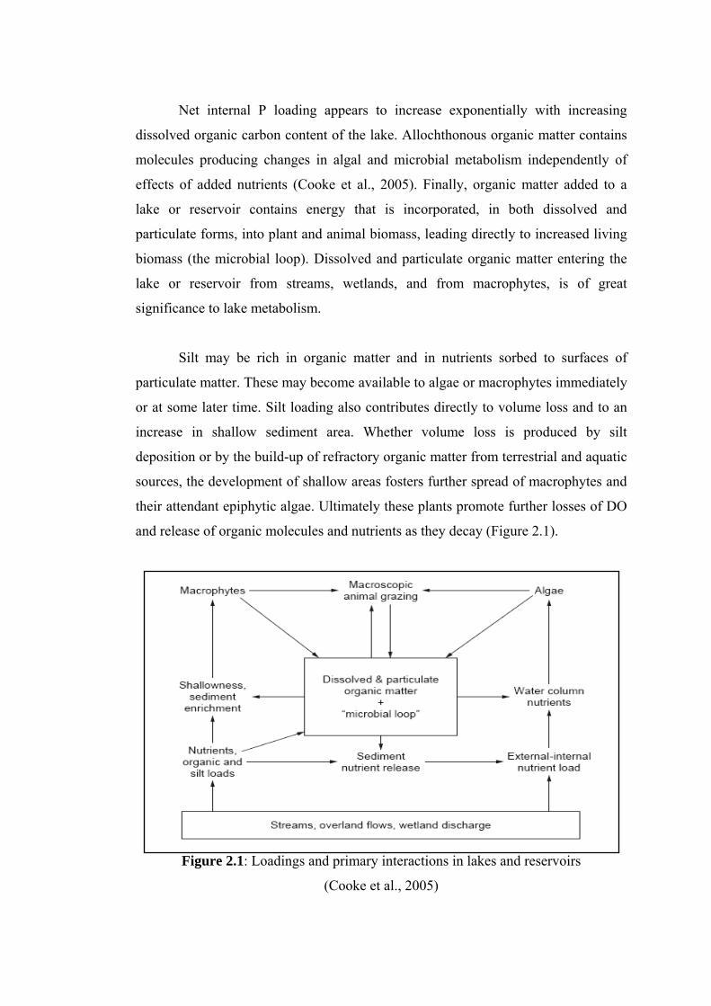
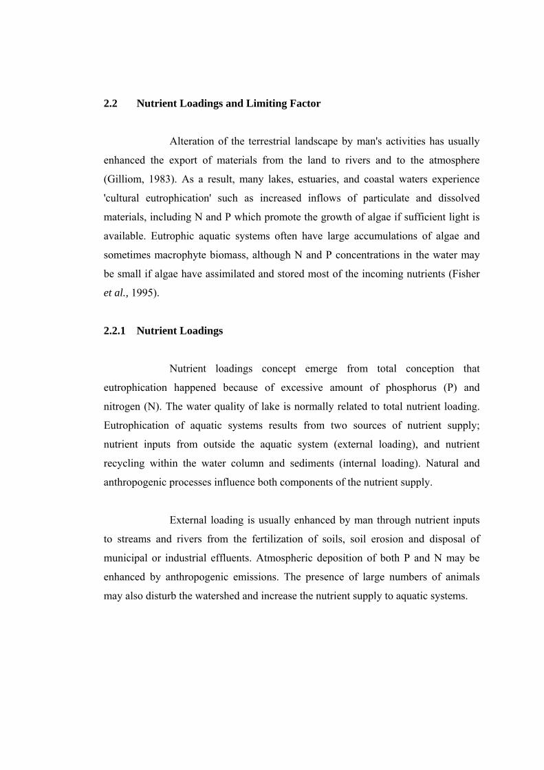
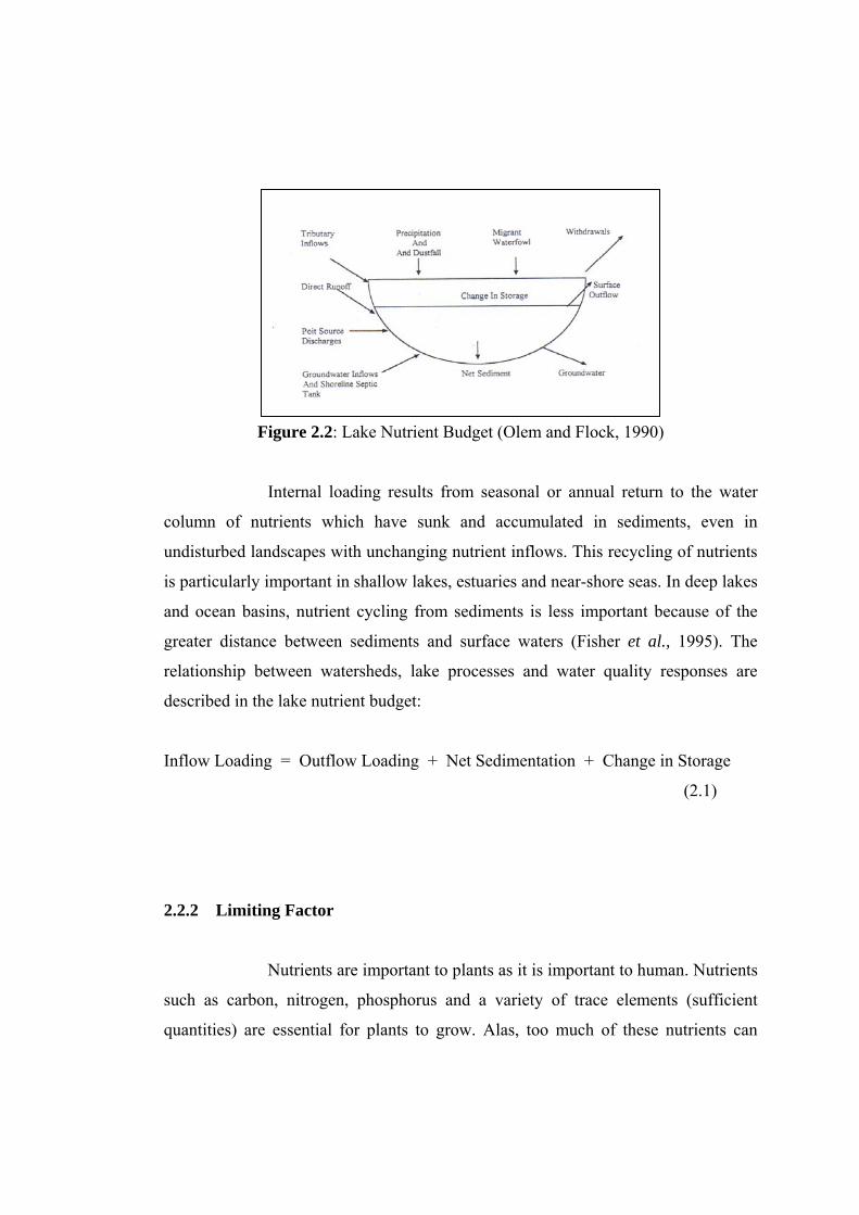
igure 2.2: Lake Nutrient Budget (Olem and Flock, 1990)

Internal loading results from seasonal or annual return to the water

trients which have sunk and accumulated in sediments, even in

ndscapes with unchanging nutrient inflows. This recycling of nutrients

important in shallow lakes, estuaries and near-shore seas. In deep lakes

ins, nutrient cycling from sediments is less important because of the

e between sediments and surface waters (Fisher et al., 1995). The

etween watersheds, lake processes and water quality responses are

e lake nutrient budget:

g = Outflow Loading + Net Sedimentation + Change in Storage

(2.1)

ng Factor

Nutrients are important to plants as it is important to human. Nutrients

n, nitrogen, phosphorus and a variety of trace elements (sufficient

essential for plants to grow. Alas, too much of these nutrients can

caused uncontrolled growth. By limiting the availability of any one nutrient, further

plant growth is prevented (Davis and Masten, 2004).

Macrophyte density, while in part related to sediment type and

composition, and to nutrient factors, is often determined by light availability. Long-

term control of algal biomass requires significant water column nutrient reduction.

Phosphorus (P) is most frequently targeted because it is usually the nutrient in

shortest supply relative to demands by algae (the limiting nutrient). Phosphorus does

not have a gaseous phase so the atmosphere is not a significant source, unlike

nitrogen or carbon. Phosphorus concentration, therefore, can be lowered significantly

by reducing loading from land and in-lake sources (Cooke et al., 2005).

There are strong relationships between inputs of P to lakes and the

biomass and productivity of phytoplankton (Dillon and Rigler, 1974) which establish

the primary importance of phosphorus limitation in freshwater lakes. This conclusion

was the basis for the recommendation that reductions in P inputs should be legislated

to control eutrophication in Malaysian lakes.

2.2.2.1 Phosphorus

Phosphorus is probably the most studied plant nutrient in freshwater

aquatic sciences. It is often found to be (and more often inferred as) the nutrient that

limits the growth and biomass of algae in lakes and reservoirs. Phosphorus in natural

waters is divided into three component parts: soluble reactive phosphorus (SRP),

soluble unreactive or soluble organic phosphorus (SUP) and particulate phosphorus

(PP) (Rigler 1973). The sum of SRP and SUP is called soluble phosphorus (SP), and

the sum of all phosphorus components is termed total phosphorus (TP). Soluble and

particulate phosphorus are differentiated by whether or not they pass through a 0.45

micron membrane filter.

Soluble reactive phosphorus (SRP) dissolves in the water and readily

aids plant growth. Its concentration varies widely in most lakes over short periods of

time as plants take it up and release it. This phosphorus fraction should consist

largely of the inorganic orthophosphate (PO4) form of phosphorus. Orthophosphate is

the phosphorus form that is directly taken up by algae, and the concentration of this

fraction constitutes an index of the amount of phosphorus immediately available for

algal growth.

Soluble unreactive phosphorus (SUP) contains filterable phosphorus

forms that do not react with the phosphorus reagents under the time and conditions of

the test. It is measured as the difference between SP and SRP. The compounds in the

SUP fraction are organic forms of phosphorus and chains of inorganic phosphorus

molecules termed polyphosphates. The size of this fraction relative to the other

phosphorus fractions is highly dependent on the type of filter used to separate the

soluble from particulate fractions.

Soluble phosphorus (SP) s measured after the digestion of the filtrate

and should contain all filterable forms of phosphorus, both organic and inorganic that

is converted to orthophosphate by the digestion process. However, the amount of

phosphorus in this filterable pool is highly dependent on the filter used. The larger

the effective pore size of the filter, the more particulate material that will pass

through the filter, be digested, and be considered "soluble."

Total phosphorus (TP) incorporates the total of all filterable and

particulate phosphorus forms mentioned above. It is probably the most often

analyzed fraction of phosphorus because it is used in a wide variety of empirical

models relating phosphorus to a wide variety of limnological variables, and the link

between phosphorus loading estimates and phosphorus content in the lake. Total

phosphorus is considered a better indicator of a lake's nutrient status because its

levels remain more stable than soluble reactive phosphorus. Total phosphorus

includes soluble phosphorus and the phosphorus in plant and animal fragments

suspended in lake water.

2.2.2.1.1 Phosphorus Cycle

Phosphorus in unpolluted waters is imported through dust in precipitation or

via the weathering of rock. Phosphorus is normally present in watersheds in

extremely small amounts, usually existing dissolved as inorganic orthophosphate,

suspended as organic colloids, adsorbed onto particulate organic and inorganic

sediment, or contained in organic water. In polluted waters, the major source of

phosphorus is from human activities. The only significant form of phosphorus

available to plants and algae is the soluble reactive inorganic orthophosphate species

(HPO42-, PO4

3-, etc.) that are incorporated into organic compounds.

During algal decomposition, phosphorus is returned to the inorganic form.

The release of phosphorus from dead algal cells is so rapid that only a small fraction

of it leaves the upper zone of a stratified lake (the epilimnion) with the settling algal

cells. However, little by little, phosphorus is transferred to the sediments; some of it

in undecomposed organic matter; some of it in precipitates of iron, aluminum, and

calcium; and some bound to clay particles. To a large extent, the permanent removal

of phosphorus from the overlying waters te the sediments depends on the amount of

iron, aluminum, calcium, and clay entering the lake along with phosphorus.

Human activities have led to a release of phosphorus from the disposal of

municipal sewage and from concentrated livestock operations. The application of

phosphorus fertilizers has also resulted in perturbations in the phosphorus cycle,

although these changes are thought to be more localized than the perturbations in the

other cycles. Phosphorus releases can have a significant effect on lake and stream

ecosystems.

2.2.2.2 Nitrate-Nitrogen

Nitrogen is an element that is found in both the living portion of our planet

and the inorganic parts of the Earth system. The nitrogen cycle is one of the

biogeochemical cycles and is very important for ecosystems. Nitrogen moves slowly

through the cycle and is stored in reservoirs such as the atmosphere, living

organisms, soils, and oceans along its way.

Most of the nitrogen on Earth is in the atmosphere. Approximately 80% of

the molecules in Earth's atmosphere are made of two nitrogen atoms bonded together

(N2). All plants and animals need nitrogen to make amino acids, proteins and DNA,

but the nitrogen in the atmosphere is not in a form that they can use. The molecules

of nitrogen in the atmosphere can become usable for living things when they are

broken apart during lightning strikes or fires, by certain types of bacteria, or by

bacteria associated with legume plants. Other plants get the nitrogen they need from

the soils or water in which they live mostly in the form of inorganic nitrate (NO3-).

Nitrogen is a limiting factor for plant growth. Animals get the nitrogen they

need by consuming plants or other animals that contain organic molecules composed

partially of nitrogen. When organisms die, their bodies decompose bringing the

nitrogen into soil on land or into the oceans. As dead plants and animals decompose,

nitrogen is converted into inorganic forms such as ammonium salts (NH4+) by a

process called mineralization. The ammonium salts are absorbed onto clay in the soil

and then chemically altered by bacteria into nitrite (NO2-) and then nitrate (NO3

-).

Nitrate is the form commonly used by plants. It is easily dissolved in water and

leached from the soil system. Dissolved nitrate can be returned to the atmosphere by

certain bacteria in a process called denitrification.

Certain actions of humans are causing changes to the nitrogen cycle and the

amount of nitrogen that is stored in reservoirs. The use of nitrogen-rich fertilizers can

cause nutrient loading in nearby waterways as nitrates from the fertilizer wash into

streams and ponds. The increased nitrate levels cause plants to grow rapidly until

they use up the nitrate supply and die. The number of herbivores will increase when

the plant supply increases and then the herbivores are left without a food source

when the plants die. In this way, changes in nutrient supply will affect the entire food

chain. Additionally, humans are altering the nitrogen cycle by burning fossil fuels

and forests, which releases various solid forms of nitrogen. Farming also affects the

nitrogen cycle. The waste associated with livestock farming releases a large amount

of nitrogen into soil and water. In the same way, sewage waste adds nitrogen to soils

and water.

2.1 Nutrients Loading Models

In view of the complexity of the transport and eutrophication processes,

various models have been developed to solve watershed and reservoir problems.

Some of them are identified as CREAMS (Chemicals, Runoff and Erosion from

Agricultural Management System) developed by Knisel (1980), ANSWERS (Areal

Non-point Source Watershed Environment Response Simulation) developed by

Beasley et. al. (1980), AGNPS (Agricultural Non-Point Source) developed by

Young et al. (1987), QUASAR (Quality Simulation Along Rivers) developed by

Whitehead et. al.(1979), VOLLENWEIDER model developed by Vollenweider

(1976) and EVENT-BASED STOCHASTIC model developed by Duckstein et. al.

(1978). The choice of the models depends on the decision to be made and the

problems to be solved (Duckstein et. al. 1978).

The non-point source simulation models vary especially in terms of their

temporal and spatial details (Srinivasan, 1992). The model could be used to simulate

short term or long term time frame or they could be based on lump or distributed

parameter approach. The lump parameter models have a limited spatial details. The

lump parameter approach applied block or average watershed physical characteristics

for one or more parameters that describe the basin as a whole. The distributed

parameter approach may include spatial variation details in the input parameters and

dependent variables. The model which allows for spatial diversity described the

watershed behavior comprehensively and is generally more accurate. The major

problems in using a distributed parameter approach is to collect all the physically-

based data required to drive the model. Besides that they are more computationally

intensive and time consuming. For a nutrient relationship study, French (1984) points

out that the short term variations are effectively treated by the dynamic distributed

models, while the long-term variations in water quality are best addressed by the

steady-state empirical lump models. The models that have dominated the non-point

modeling arena especially for agricultural areas will be discussed below.

2.3.1 CREAMS

The CREAMS (Chemicals, Runoff and Erosion from Agricultural

Management System) model was developed by the United States Department of

Agriculture –Agricultural Research Service (USDA-ARS) (Donigian and Wayne,

1991) . This model was developed based on the earlier version initiated by Knisel

(1980) for analysis of agricultural best management practices for pollution control.

Specifically this physically-based and lumped parameter model was applied for

predicting runoff, erosion and chemical transport from field-sized agricultural areas.

CREAMS could predict the fate and transport of chemicals in the soil such as total

phosphorus and total nitrogen from the agricultural field-sized area. It could also

predict erosion, sediment yield, the distribution of the primary sediment particles and

sediment-bound nitrogen and phosphorus (Srinivasan, 1992). CREAMS uses a

representative slope flow path to describe the field-sized area. The sediment and

transport equations will predict the sediment movement for the slope flow path

endured. The CREAMS model could determine the storm loads and average

concentrations of sediment- associated and dissolved chemicals in runoff (Donigian

and Wayne, 1991). The CREAMS model could also simulate the runoff discharges

on a daily basis, erosion from field-sized areas and land surface and soil chemical

processes. The CREAMS model could also simulate various management activities

which could be defined by the user such as soil incorporation of pesticides, animal

waste management, agricultural practices which include minimum tillage and

terracing and aerial spraying. CREAMS could be used for long term simulations

(usually two to fifty years) and also for simulating single storms.

The CREAMS model consists of three main components; they are

hydrologic, erosion or deposition and nutrients movements or chemistry submodels.

CREAMS is a product of the agricultural research community with specific emphasis

on representing land surface, soil profile and field scale processes (Donigian and

Wayne, 1991). CREAMS allows a very detailed representation of the processes

involved in estimating nutrient losses in runoff and through leaching. The chemical

processes detailed representation include the sorption or desorption, plant uptake,

mineralization and nitrification which eventually would control the fate and

migration of chemicals in the soil. The land surface detailed representation include

the field terraces, drainage systems, field topography and associated sediment

erosion processes. Daily erosion and sediment yield, including particle size

distribution are estimated at the edge of the field. The detailed hydrologic option is

also available which include short term interval rainfall and the popular Soil

Conservation Service (SCS) Curve Number procedure. Runoff volume, peak flow,

infiltration, evapotranspiration, soil water content and percolation are computed on a

daily basis. The structure and the processes involved in the CREAMS model are

described in Figure 2.6.

CREAMS advantages and strength are mainly focused on the calibration

procedure which are not necessarily required in their modeling effort (Donigian and

Wayne, 1991). The model provides an accurate representation of the various soil

processes. Most of the CREAMS parameter values are physically measurable.

Besides a complex field-sized watershed can be represented with minimum input

details when using CREAMS. When the input data needed by the model could not be

provided, default values for input variables which are available (except for those

describing the slope) can be used for estimating erosion. However, the results

obtained by using the default values will likely be less accurate (Srinivasan, 1992).

CREAMS’s weaknesses are mainly focused on the variability of the results which

could only be represented in the downslope direction and information is not provided

during a storm (Srinivasan, 1992). Another weakness of CREAMS is that it is unable

to properly simulate areas with a high water tables and a significant interflow

component for surface runoff. As CREAMS is a continuous simulation model, the

data needed are detail and extensive.

CREAMS has been applied in a wide variety of hydrologic and water quality

studies. Sapek and Sapek (1993) studied the application of the CREAMS model to

forecast nitrate and chloride leaching from grassland near Warsaw, Poland. Their

results ascertained that the CREAMS is a proper tool for forecasting nitrogen balance

on permanent grassland, particularly due to nitrate leaching. Gouy and Belamie

(1993) applied the CREAMS pesticides transfer submodel at a rainfall simulation

scale. The pesticide sub-model of CREAMS was tested to describe the pesticide

transfer into runoff generated by a rainfall simulation. Adsorption coefficient, Kd,

was found to be a sensitive parameter of the model. Mean Kd measured in the runoff

of a rainfall simulation was considerably greater than the reported values (Sapek and

Sapek, 1993), especially for the low suspended particle loads. Williams and Nicks

(1993) studied the modeling approach to evaluate best management practices for

cropland in Durand, USA. The best management practice evaluated was vegetative

filter strips, 20m to 30m wide established alongside streams and creeks adjacent to

cropland. The studies outcome indicated that filter strips generally reduced sediment

and sediment-associated nutrients by 10 to 80% depending on site features and

characteristics. Overall filter strips reduced sediment by 56 % and sediment

associated nutrients by 50%.

2.3.2 ANSWERS

ANSWERS (Areal Non-point Source Watershed Environment Response

Simulation) developed by Beasley et. al. (1980) is primarily a distributed parameter,

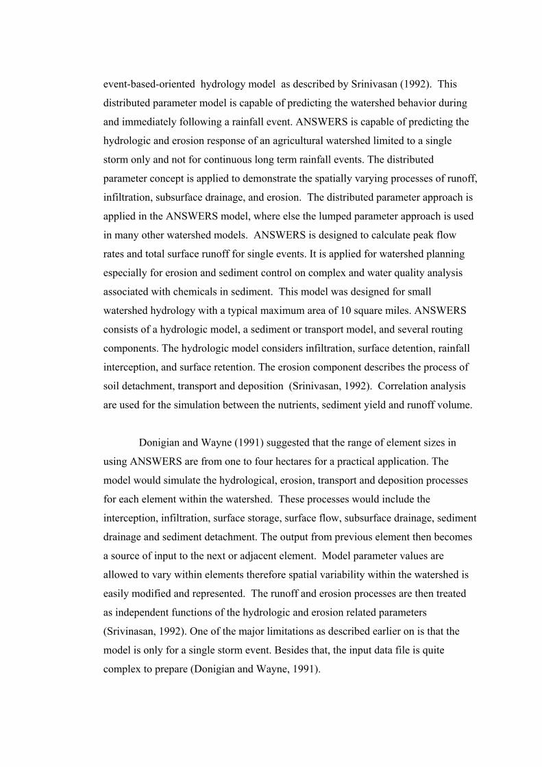
event-based-oriented hydrology model as described by Srinivasan (1992). This

distributed parameter model is capable of predicting the watershed behavior during

and immediately following a rainfall event. ANSWERS is capable of predicting the

hydrologic and erosion response of an agricultural watershed limited to a single

storm only and not for continuous long term rainfall events. The distributed

parameter concept is applied to demonstrate the spatially varying processes of runoff,

infiltration, subsurface drainage, and erosion. The distributed parameter approach is

applied in the ANSWERS model, where else the lumped parameter approach is used

in many other watershed models. ANSWERS is designed to calculate peak flow

rates and total surface runoff for single events. It is applied for watershed planning

especially for erosion and sediment control on complex and water quality analysis

associated with chemicals in sediment. This model was designed for small

watershed hydrology with a typical maximum area of 10 square miles. ANSWERS

consists of a hydrologic model, a sediment or transport model, and several routing

components. The hydrologic model considers infiltration, surface detention, rainfall

interception, and surface retention. The erosion component describes the process of

soil detachment, transport and deposition (Srinivasan, 1992). Correlation analysis

are used for the simulation between the nutrients, sediment yield and runoff volume.

Donigian and Wayne (1991) suggested that the range of element sizes in

using ANSWERS are from one to four hectares for a practical application. The

model would simulate the hydrological, erosion, transport and deposition processes

for each element within the watershed. These processes would include the

interception, infiltration, surface storage, surface flow, subsurface drainage, sediment

drainage and sediment detachment. The output from previous element then becomes

a source of input to the next or adjacent element. Model parameter values are

allowed to vary within elements therefore spatial variability within the watershed is

easily modified and represented. The runoff and erosion processes are then treated

as independent functions of the hydrologic and erosion related parameters

(Srivinasan, 1992). One of the major limitations as described earlier on is that the

model is only for a single storm event. Besides that, the input data file is quite

complex to prepare (Donigian and Wayne, 1991).

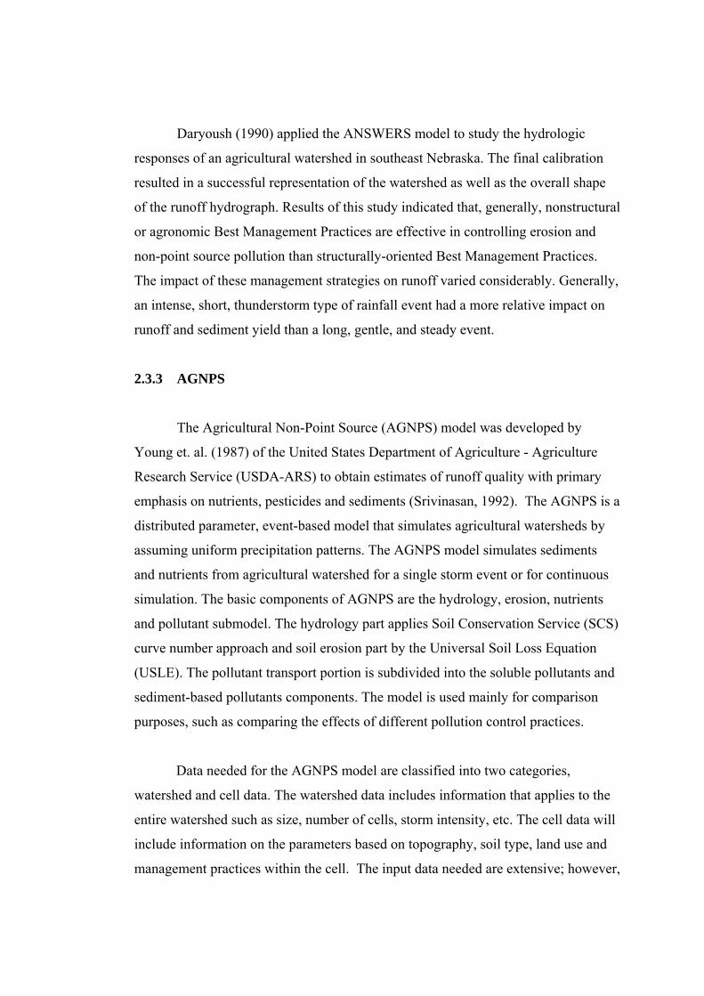
Daryoush (1990) applied the ANSWERS model to study the hydrologic

responses of an agricultural watershed in southeast Nebraska. The final calibration

resulted in a successful representation of the watershed as well as the overall shape

of the runoff hydrograph. Results of this study indicated that, generally, nonstructural

or agronomic Best Management Practices are effective in controlling erosion and

non-point source pollution than structurally-oriented Best Management Practices.

The impact of these management strategies on runoff varied considerably. Generally,

an intense, short, thunderstorm type of rainfall event had a more relative impact on

runoff and sediment yield than a long, gentle, and steady event.

2.3.3 AGNPS

The Agricultural Non-Point Source (AGNPS) model was developed by

Young et. al. (1987) of the United States Department of Agriculture - Agriculture

Research Service (USDA-ARS) to obtain estimates of runoff quality with primary

emphasis on nutrients, pesticides and sediments (Srivinasan, 1992). The AGNPS is a

distributed parameter, event-based model that simulates agricultural watersheds by

assuming uniform precipitation patterns. The AGNPS model simulates sediments

and nutrients from agricultural watershed for a single storm event or for continuous

simulation. The basic components of AGNPS are the hydrology, erosion, nutrients

and pollutant submodel. The hydrology part applies Soil Conservation Service (SCS)

curve number approach and soil erosion part by the Universal Soil Loss Equation

(USLE). The pollutant transport portion is subdivided into the soluble pollutants and

sediment-based pollutants components. The model is used mainly for comparison

purposes, such as comparing the effects of different pollution control practices.

Data needed for the AGNPS model are classified into two categories,

watershed and cell data. The watershed data includes information that applies to the

entire watershed such as size, number of cells, storm intensity, etc. The cell data will

include information on the parameters based on topography, soil type, land use and

management practices within the cell. The input data needed are extensive; however,

it could be obtained through visual field observations, topographic and soil maps and

from various publications, tables and graphs (Donigian and Wayne, 1991).

Meteorologic data consisting of daily rainfall is needed for the hydrologic

simulation. The model requires a total of 22 parameters for execution. Output

parameters can be examined for a single cell or for the entire watershed. The

nutrients, sediment and runoff estimates produced by the AGNPS can be examined

for a selected areas within the watershed or for a the whole watershed. In general,

AGNPS performed well and provide reasonably satisfactory results.

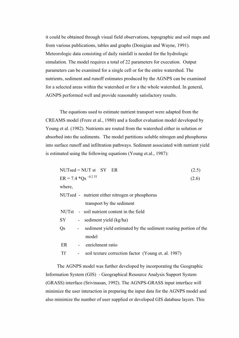
The equations used to estimate nutrient transport were adapted from the

CREAMS model (Frere et al., 1980) and a feedlot evaluation model developed by

Young et al. (1982). Nutrients are routed from the watershed either in solution or

absorbed into the sediments. The model partitions soluble nitrogen and phosphorus

into surface runoff and infiltration pathways. Sediment associated with nutrient yield

is estimated using the following equations (Young et.al., 1987):

NUTsed = NUT st SY ER (2.5)

ER = 7.4 *Qs –0.2 Tf (2.6)

where,

NUTsed - nutrient either nitrogen or phosphorus

transport by the sediment

NUTst - soil nutrient content in the field

SY - sediment yield (kg/ha)

Qs - sediment yield estimated by the sediment routing portion of the

model

ER - enrichment ratio

Tf - soil texture correction factor (Young et. al. 1987)

The AGNPS model was further developed by incorporating the Geographic

Information System (GIS) - Geographical Resource Analysis Support System

(GRASS) interface (Srivinasan, 1992). The AGNPS-GRASS input interface will

minimize the user interaction in preparing the input data for the AGNPS model and

also minimize the number of user supplied or developed GIS database layers. This

interface will prepare the input data with only 8 basic GIS database layers supplied

by the user and with minimal user interaction compared to the 22 different data

required by the basic AGNPS model for each cell (Srinivasan, 1992). There are 5

input parameters needed for the whole watershed which will be supplied by the user.

The major asset of the GIS approach is that it will automatically extract the required

information to calculate the model data. The process of extracting data from the

map sources has been divided into two major sections:

i) Topography related data

ii) Soil type and land cover related data. The topography related variables will include the receiving cell flow direction. The soil type and land cover related data will include the soil erodibility (K) factor, Manning’s n and SCS curve number (Srinivasan, 1992).

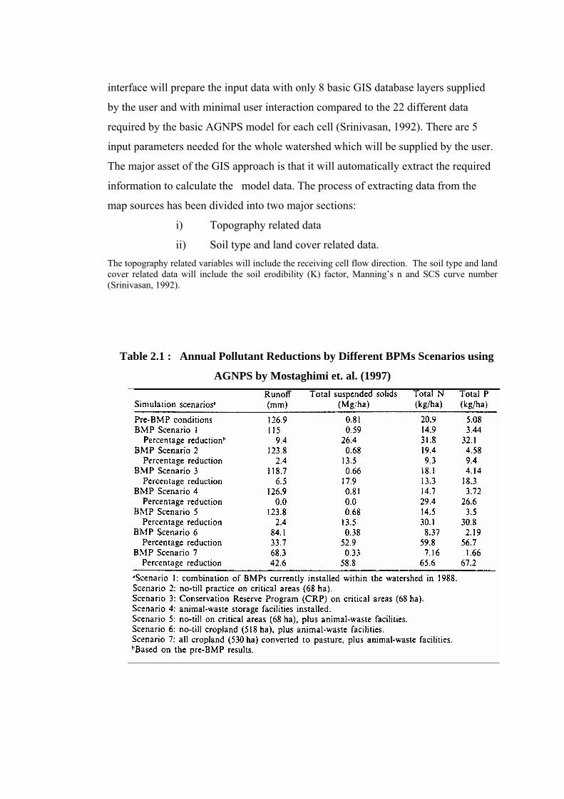
Table 2.1 : Annual Pollutant Reductions by Different BPMs Scenarios using

AGNPS by Mostaghimi et. al. (1997)

Mostaghimi et. al. (1997) applied the AGNPS model for assessing

management alternatives in a small agricultural watershed on the water quality and

quantity in the Piedmont Region of Virginia, USA. The runoff, sediment yield and

nutrient loadings predicted by the AGNPS model compared favorably with the

observed values. A better result was found for runoff but less favorable for peak

rates, sediment or nutrient yields. Mostaghimi et. al. (1997) applied the annualization

procedure suggested by Koelliker and Humbert (1989) to convert event-based

simulation result into a long-term impacts of best management practices (BMPs).

The procedure takes into account rainfall amount frequency analysis and the

corresponding rainfall erosivity indices. The relative errors of the annualization

procedure was 23.5, 14.3 and 8.9 % for sediment yield, nitrate and phosphorus

loadings respectively. The model was also used to simulate the effects of seven

different BMPs scenarios on the watershed. The reduction rates in simulated

pollutant loadings and costs for BMPs implementation were used to identify the

appropriate BMPs for the watershed. Their results also indicated that the installation

of BMPs on critical areas may be cost effective. The most critical areas could be

treated first and then BMPs could be implemented on the less critical areas until the

reduction goals are met. The annual pollutant reductions by different BMP scenarios

studied by Mostaghimi et. al (1997) are shown in Table 2.1. However, they

cautioned that the input data for this model is very time consuming and a lot of

difficulties arise in determining the accuracy of the output values.

2.3.4 QUASAR

QUASAR (Quality Simulation Along Rivers) was developed by Whitehead

et. al.(1979) to assess the environmental impact of pollutants on river water quality.

The model was originally developed with the primary objective of simulating the

dynamic behavior of flow and water quality along a river system (Whitehead and

Young, 1979). QUASAR performs a mass balance of flow and water quality

sequentially down a river system. The model combines inputs from tributaries,

groundwater and point and non-point sources to calculate the flow and river water

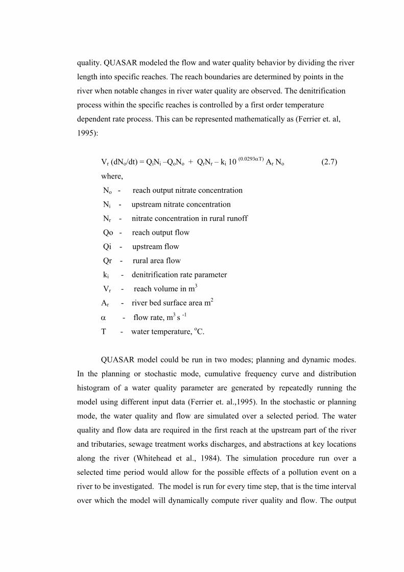
quality. QUASAR modeled the flow and water quality behavior by dividing the river

length into specific reaches. The reach boundaries are determined by points in the

river when notable changes in river water quality are observed. The denitrification

process within the specific reaches is controlled by a first order temperature

dependent rate process. This can be represented mathematically as (Ferrier et. al,

1995):

Vr (dNo/dt) = QiNi –QoNo + QrNr – ki 10 (0.0293αT) Ar No (2.7)

where,

No - reach output nitrate concentration

Ni - upstream nitrate concentration

Nr - nitrate concentration in rural runoff

Qo - reach output flow

Qi - upstream flow

Qr - rural area flow

ki - denitrification rate parameter

Vr - reach volume in m3

Ar - river bed surface area m2

α - flow rate, m3 s -1

T - water temperature, oC.

QUASAR model could be run in two modes; planning and dynamic modes.

In the planning or stochastic mode, cumulative frequency curve and distribution

histogram of a water quality parameter are generated by repeatedly running the

model using different input data (Ferrier et. al.,1995). In the stochastic or planning

mode, the water quality and flow are simulated over a selected period. The water

quality and flow data are required in the first reach at the upstream part of the river

and tributaries, sewage treatment works discharges, and abstractions at key locations

along the river (Whitehead et al., 1984). The simulation procedure run over a

selected time period would allow for the possible effects of a pollution event on a

river to be investigated. The model is run for every time step, that is the time interval

over which the model will dynamically compute river quality and flow. The output

values are used in generating profiles of water quality parameters along the river at a

given time or in generating time series data at a specified location. The simulated and

observed river flows at the downstream boundary is necessary for the loading

estimation. The simulated daily nitrate concentrations and observed monthly are

obtained from the study.

Ferrier et. al. (1995) applied the QUASAR model to investigate the impact of land

use change and climate change on NO3-N in the River Don, North East Scotland.

They investigated a range of land use scenarios and climate effects to provide a long

term view of nitrate nitrogen concentrations in the river in future years. The primary

data available for the study were the river reach length and cross section, maximum

and minimum temperatures and flow discharges. Flow discharges were monitored

continuously at a number of locations on the main river channel by the North East

River Purification Board (NERPB), Scotland. Seasonal variations in discharge are

apparent, low flows being associated with summer months and high flows as a result

of autumn and spring snowmelt. The river water samples were collected

approximately monthly over the 11 years period (1980-1990) as part of NERPB’s

routine water quality control and monitoring duty. Ferrier et. al (1995) identified

three reach structure with the non-point inputs along the river system treated as

single point input per reach.

2.3.6 Universal Soil Loss Equation (USLE)

The USLE, developed by Wischmeier and Smith (1962) is the most widely

used and accepted erosion model (Williams and Hann, 1978). The USLE can be

used to predict long-term average annual sediment yields for watersheds by applying

a delivery ratio. USLE can also be used for pollution loading estimation by

multiplying the sediment yield estimated with the concentration of pollutant in soil.

USLE has been used to provide specific and reliable guides for selecting appropriate

erosion control practices for farmlands and construction areas (e.g. Morgan, 1986a).

This empirically based model, compute soil erosion by assigning values to indices

that represent the major factors of climate, soil, topography and land use. Other

applications of the equation have been in determining upland erosion for reservoir

sedimentation and stream loading, control of pollution from cropland, and alternative

land use and treatment combinations (Morgan, 1986a).

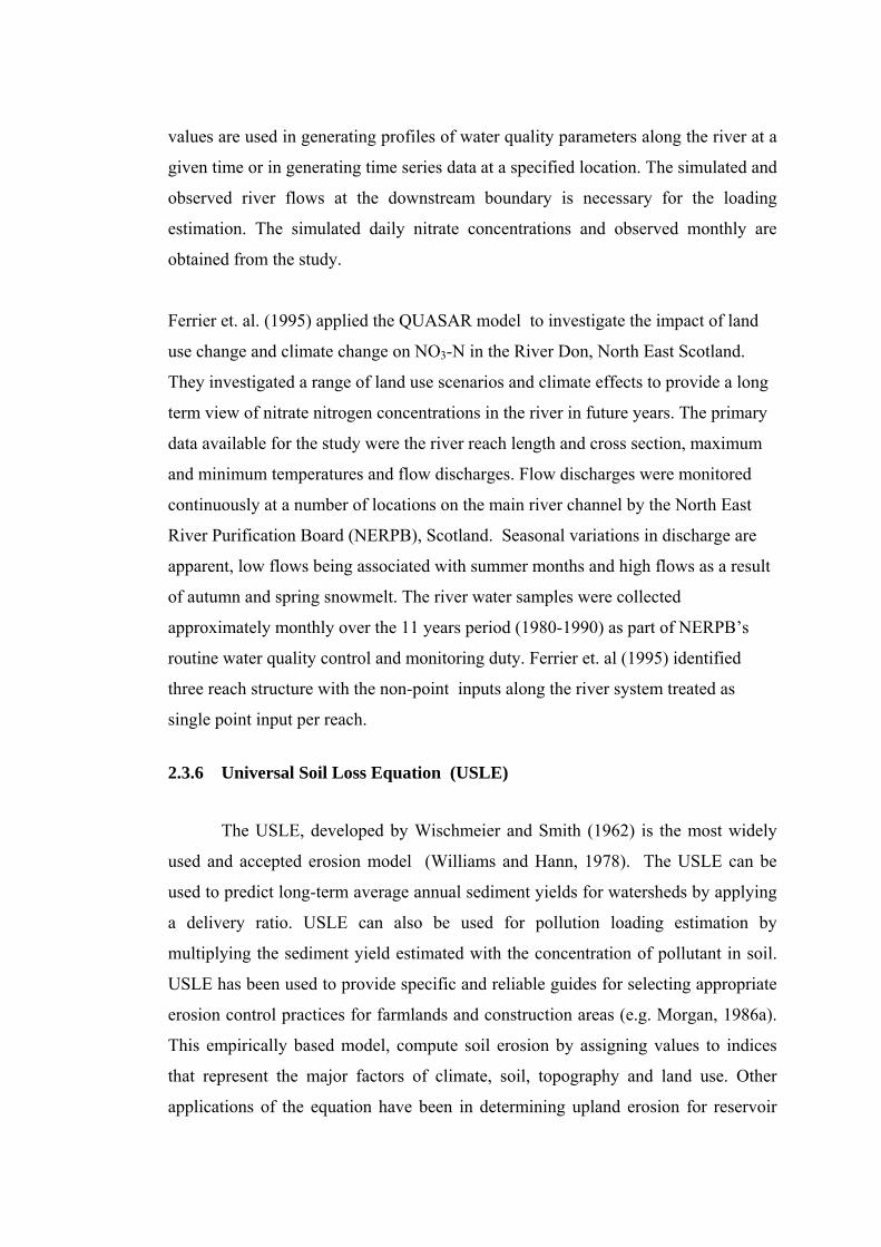
The Universal Soil Loss Equation (Wischmeier and Smith, 1962) expresses

the relationship between various factors quantitatively in the following form:

A = R.K.L.S.C.P (2.11)

where,

A = mean annual soil erosion loss ( tons/ha/year)

R = rainfall erosivity index ( tons/ha/ ( in/hr ))

K = soil erodibility factor (tons/ ha/year per unit R )

L = slope length factor (dimensionless)

S = slope steepness factor (dimensionless)

C = crop management factor (dimensionless)

P = erosion control practice factor (dimensionless)

In metric units,

A(tons/ha/year) = R(J/ha) x K (tons/J/year) LSCP (2.12)

Note: ha - hectar

J - Joule (Nm or kg m2/s2)

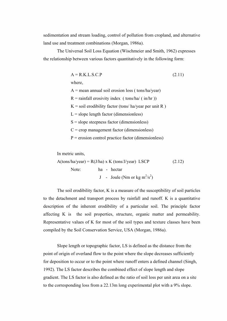
The soil erodibility factor, K is a measure of the susceptibility of soil particles

to the detachment and transport process by rainfall and runoff. K is a quantitative

description of the inherent erodibility of a particular soil. The principle factor

affecting K is the soil properties, structure, organic matter and permeability.

Representative values of K for most of the soil types and texture classes have been

compiled by the Soil Conservation Service, USA (Morgan, 1986a).

Slope length or topographic factor, LS is defined as the distance from the

point of origin of overland flow to the point where the slope decreases sufficiently

for deposition to occur or to the point where runoff enters a defined channel (Singh,

1992). The LS factor describes the combined effect of slope length and slope

gradient. The LS factor is also defined as the ratio of soil loss per unit area on a site

to the corresponding loss from a 22.13m long experimental plot with a 9% slope.

Slope gradient in the field or segment slope is usually expressed as a percentage. The

development of segment slope was based on a standard plot length of 22.13 m

(Wischmeier and Smith, 1962).

The cover and management factor, C is defined as the ratio of soil loss from

land under specified crop or mulch conditions to the corresponding loss from tilled

and bare soil. This cropping management factor represents the ratio of soil loss from

a specific cropping or cover condition to the soil loss from a tilled, continuous fallow

condition for the same soil, slope and same rainfall (Wischmeier and Smith, 1978).

This factor measures the combined effect of all the interrelated cover and

management variables including the type of vegetation, plant spacing, the stand, the

quality of growth, crop sequence, tillage practices, crop residues, incorporated

residues, land use residue and fertility treatments (Singh, 1992). Crops can be grown

continuously or rotated with other crops. Soil loss and sediment yield can be reduced

if the particular site is covered with vegetation. The greatly expanded tables of C

factor values were presented by Wischmeier (1960), Wischmeier and Smith (1962),

Roose (1977) and Morgan (1986a).

Support practice factor, P is defined as the ratio of soil loss with a given

surface condition to soil loss with up and down hill culture (Wischmeier and Smith,

1978). Important cropland practices are contour tillage, strip cropping on the contour

and terrace systems. Practices that reduce the velocity of runoff and the tendency of

runoff to flow directly down slope reduce the P factor. Since slope length influences

the effectiveness of contouring, the P values are based on maximum slope lengths.

Mitchell and Bubenzer (1980) indicated conservation tillage, crop rotations, fertility

treatments and the retention of residues are important erosion control practices. They

also indicated that the P factor is most effective for the 3-8% slope range and values

increase as the slope increases.

USLE had been modified and renamed in several versions such as MUSLE

(Modified Universal Soil Loss Equation) and RUSLE (Revised Universal Soil Loss

Equation). The USLE was not designed for application to individual storms and is

therefore, not appropriate for individual storm water quality modeling. The USLE

was modified by Williams (1975a) for watershed application by replacing the rainfall

energy factor with a runoff factor. This modified version called MUSLE increased

sediment-yield-prediction accuracy, eliminated the need for delivery ratios, and is

applicable to individual storms. The MUSLE was combined with the modified SCS

water-yield model to form a daily runoff-sediment prediction model (Williams and

Berndt, 1976). The MUSLE is useful in predicting sediment yield from small

watersheds (< 40 km2) however sediment routing is needed to maintain prediction

accuracy on large watersheds with non-uniformly distributed sediment sources

(Williams and Hann,1978). A sediment routing model was developed for large

agricultural watersheds (Williams, 1975b) and has had limited testing.

Although USLE was widely used, it has some important limitations. The data

base used in developing the USLE was collected on the east of the Rocky Mountains,

therefore its limitation when applying in the other parts of the world especially in the

arid and tropical region must be recognized (Simons et. al.,1982). Many arid regions

in the western United States gets a large percentage of rainfall in the form of high

intensity, short-duration thunderstorms. As this in not the case in the eastern United

States, the effect of this type of rainfall cannot be totally incorporated. The USLE

can be helpful for prediction of sediment contributions from these sources to

downstream water bodies, but the limitations in terms of the type of erosion

applicable must be recognized. The USLE is designed to predict average annual soil

loss by sheet and rill erosion on unsloped areas such as farmland and agricultural

areas. Its predictions do not include sediment contributions from gully erosion or

landslides. Since it was designed for sheet and rill erosion, it should not be used to

estimate sediment yield from drainage basins. The soil loss estimated using USLE

does not include factors to account for sediment losses or gains between the field and

stream or reservoir. These items must be evaluated separately. The USLE was

developed from data taken from small plots. Because of its regression nature, results

become suspicious when applied to much larger areas. It has been developed for

materials in the range of 1mm or finer, and does not predict the yield of larger

sediment sizes (Simons et. al, 1982).

2.3.7 Event-Based Stochastic Model

The Event-Based Stochastic Model was developed by Duckstein et. al.

(1978) for phosphorus loadings estimation. This Event-Based Stochastic Model

recognized the stochastic nature of nutrient input and the probabilistic description of

phosphorus loadings in terms of their frequency and the uncertainty (Duckstein et. al.

1978). The model encoded the uncertainty of phosphorus loadings in terms of mean,

variance and probability density function. The model accounts separately the two

different forms of phosphorus; dissolved phosphorus and sorbed phosphorus.

Phosphorus input is separated into the two components to account for the two

different forms of transport of phosphorus from the watershed into the lake.

The elements of the Event-Based Stochastic Model are summarized as

follows:

i) Random precipitation events which lead to transport of phosphorus

by the two associated mechanisms (runoff volume and sediment yield)

ii) Source of phosphorus, dissolved and sediment phosphorus for a given

watershed

iii) Dissolved phosphorus loadings, a function of runoff volume

iv) Sediment or particulate phosphorus loadings, a function of sediment

yield

v) Total seasonal loadings of dissolved phosphorus and sediment

phosphorus.

This Event-Based Stochastic Model is further elaborated in Chapter 4.

2.3 Nutrient Loading Model

There are several research and method that contributes to the

development of nutrient loading evaluation. The most useful and extensively being

used is the model introduced by Richard A. Vollenweider. The model has been

widely applied in many studies because of its proper definition of lake eutrophication

process.

2.3.1 Vollenweider Model

The Vollenweider Model is a useful tool in determining the trophic

state of water body based on phosphorus loading (P-loading) and the water depth.

The model was originally developed for application to deep, glacial lakes located in

the northern hemisphere (Vollenweider, 1968). Vollenweider radically changed our

view of lakes when he emphasized the importance of nutrient inputs from the

watershed in the determination of the concentration of nutrients and, ultimately, the

density of algae in the lake. He was able to convince a new generation of

limnologists to look to the watershed to understand the lake only after 50 years later.

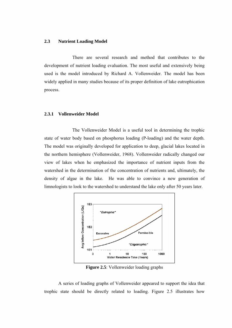
Figure 2.5: Vollenweider loading graphs

A series of loading graphs of Vollenweider appeared to support the idea that

trophic state should be directly related to loading. Figure 2.5 illustrates how

investigators with loading data are tempted to simply classify the trophic state of a

lake. In this case, trophic state is determined by plotting "Average inflow

concentration," which is calculated by dividing loading (L) by water loading (qs),

against hydrologic constraints (water residence time). The “Permissible” line is the

boundary between oligotrophy and mesotrophy, and “Excessive” line, the boundary

between mesotrophy and eutrophy (Vollenweider 1976).

The Vollenweider model is based on a five year study involving the

examination of phosphorus load and response characteristics for about 200 water

bodies in 22 countries in Western Europe, North America, Japan and Australia.

Vollenweider, working on the Organization for Economic Cooperation and

Development (OECD) Eutrophication Study, developed a model describing the

relationship of phosphorus load and the relative general acceptability of the water for

recreational use. He found that when the annual phosphorus load to a lake is plotted

as a function of the quotient of the mean depth and hydraulic residence time, lakes

which were eutrophic tended to cluster in one area and oligotrophic lakes in another

(Vollenweider, 1975).

Vollenweider developed a statistical relationship between areal annual

phosphorus loading (Lp) to a lake normalized by mean depth (Z) and hydraulic

residence time (T), to predict lake phosphorus concentration (P). The general steady-

state equation for phosphorus loading by Vollenweider (1976) can be written as:

[ ] INTi

n

iip LPQL += ∑

=1

(2.1)

where

pL is the loading of phosphorus per unit area per year ( ) 12 −− yrmgm

iQ represents the amount of water supplied by each input

iP is the mean P concentration of dissolved and sediment-bound phosphorus

(external loading)

INTL is the loading from the lake sediments to the water column (internal

loading)

Internal loadings of P from lake sediments to the water column are difficult to

measure. Assuming negligible , the equation becomes: INTL

( )whtotp TqPL +⋅⋅= 1 (2.2)

where

pL is the loading of phosphorus per unit area per year (mgm-2 yr-1)

totP is the mean P concentration of dissolved and sediment phosphorus in the

water body

hq is the hydraulic loading (myr-1)

wT is the mean residence time of water in the lake (yr)

As a general rule, the critical P values that will convert the

oligotrophic state to the mesotrophic state is Lg /10µ . Thus the equation (2.2) can be

transformed into:

( )hhc qzqL +⋅= 110 (2.3)

where

z is the lake mean depth (m)

The phosphorus loading Y tons year-1 is obtained by multiplying the loading

L tons m-2 yr-2 with the surface area of the reservoir.

CHAPTER 3

METHODOLOGY 3.1 Site description

The Layang reservoir in Layang catchment area can be divided into two

reservoirs, which are Hulu Layang reservoir and Hilir Layang reservoir. The

reservoir is located in Masai, around 40 km travel distance from Johor Bahru city.

The maximum altitude is 160 m while minimum altitude is 30 m above the mean sea

level. The areal coverage for the catchment area approximately yields within

coordinates of latitudes 1o 30’ N until 1o 36’ N and longitudes 103o 50’ E until 104o

00’ E.

Hilir Layang reservoir is situated on the east side of Hulu Layang reservoir.

The drainage basin for Hilir Layang reservoir is 20.5 km2. The total drainage basin

for both Hulu and Hilir reservoir is 50.5 km2. The water outflow from both

catchments is approximately 40 mega gallons per day. The outflow rate of water

from the intake tower to the water treatment plant is 28.5 mega gallon per day (Sek,

1997).

The activities near the Layang river watershed mostly are villages, plantation

and agricultural estates. These areas are most likely to produce wastes that will

contribute to the discharge into the Layang river watershed when large amounts of

fertilizers and pesticides were used in these areas. In other words, these are the

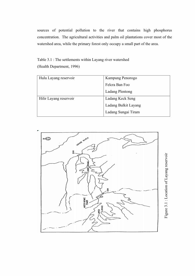
sources of potential pollution to the river that contains high phosphorus

concentration. The agricultural activities and palm oil plantations cover most of the

watershed area, while the primary forest only occupy a small part of the area.

Table 3.1 : The settlements within Layang river watershed

(Health Department, 1996)

Hulu Layang reservoir

Kampung Penorogo

Felcra Ban Foo

Ladang Plentong

Hilir Layang reservoir

Ladang Keck Seng

Ladang Bulkit Layang

Ladang Sungai Tiram

Figu

re 3

.1 :

Loca

tion

of L

ayan

g re

serv

oir

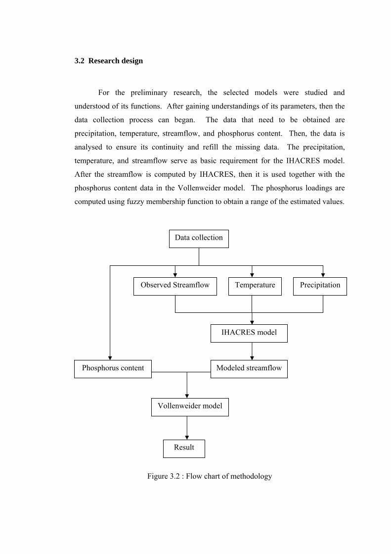
3.2 Research design

For the preliminary research, the selected models were studied and

understood of its functions. After gaining understandings of its parameters, then the

data collection process can began. The data that need to be obtained are

precipitation, temperature, streamflow, and phosphorus content. Then, the data is

analysed to ensure its continuity and refill the missing data. The precipitation,

temperature, and streamflow serve as basic requirement for the IHACRES model.

After the streamflow is computed by IHACRES, then it is used together with the

phosphorus content data in the Vollenweider model. The phosphorus loadings are

computed using fuzzy membership function to obtain a range of the estimated values.

Temperature Observed Streamflow Precipitation

Phosphorus content Modeled streamflow

IHACRES model

Vollenweider model

Data collection

Result

Figure 3.2 : Flow chart of methodology

3.3 Data collection

For the purpose of this study, visitations will be made to the site to take

measurements and to obtain the water samples for testing. Three visits were

launched to the site with the help from technical assistants of hydraulic and

hydrology department. The visits were conducted on 21/12/2006, 10/01/2007 and

21/02/2007.

3.3.1 Water sampling

Water samples can be taken with the help of a tool called water sampler. The

commonly used water sampler consists of a cylindrical tube with a stopper on each

end that is controlled by a closing device. Water sampler can be used to take water

samples at any desired depths, which make it handy when the stream or river only

can be reached from higher grounds for example bridges. In order to use it, the tube

is lowered into the water at the desired depth with the rubber plugs open. A weight

is then dropped down the supporting cord to trip the closing mechanism, which will

close the stoppers and trap water inside the tube.

3.3.2 Streamflow measurement

The velocity-area method is used in this study to determine the streamflow of the

river. In order to use this method for the determination of discharge,

measurements of stream velocity, depth of flow and the distance across the

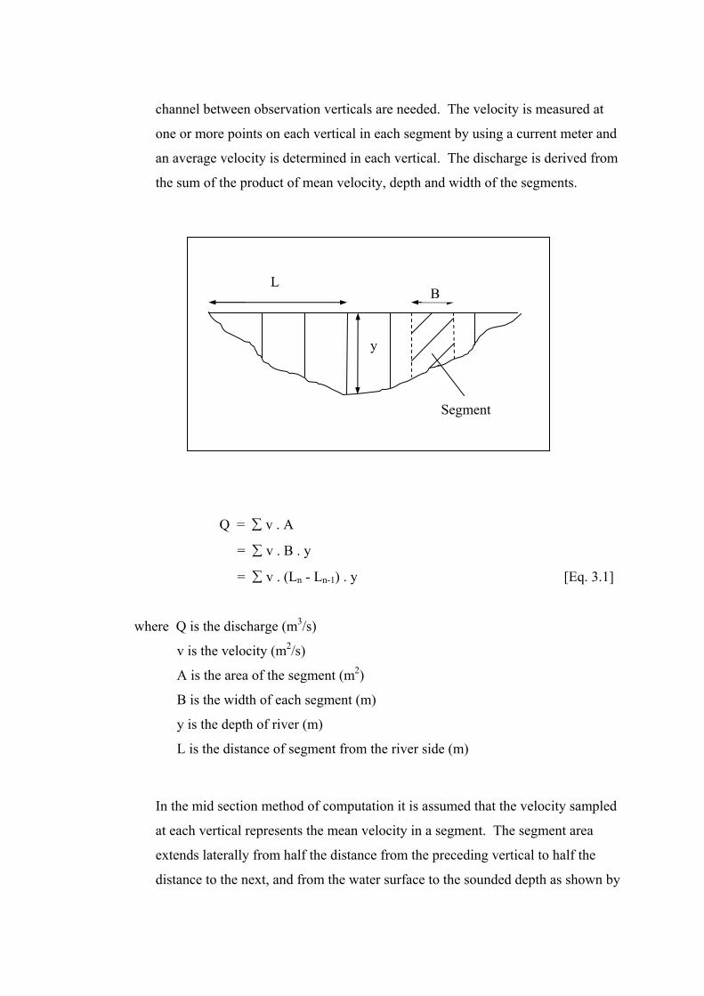
channel between observation verticals are needed. The velocity is measured at

one or more points on each vertical in each segment by using a current meter and

an average velocity is determined in each vertical. The discharge is derived from

the sum of the product of mean velocity, depth and width of the segments.

y

Segment

BL

Q = ∑ v . A

= ∑ v . B . y

= ∑ v . (Ln - Ln-1) . y [Eq. 3.1]

where Q is the discharge (m3/s)

v is the velocity (m2/s)

A is the area of the segment (m2)

B is the width of each segment (m)

y is the depth of river (m)

L is the distance of segment from the river side (m)

In the mid section method of computation it is assumed that the velocity sampled

at each vertical represents the mean velocity in a segment. The segment area

extends laterally from half the distance from the preceding vertical to half the

distance to the next, and from the water surface to the sounded depth as shown by

the hatched area in figure. The segment discharge is then computed for each

segment and these are summed to obtain the total discharge (Herschy, 1995).

3.3.3 Phosphorus testing

The water samples taken from site were brought back to the lab for testing of

the phosphorus concentration in the water samples. The samples were tested using

reagent phosVer 3 phosphates and DR4000 spectrophotometer (Hach Co. CO80539-

9987, USA). The phosphorus content is indicated in mg/l.

3.4 Vollenweider model

From studies and research by many researchers in the past, they discovered

that the phosphorus is the limiting nutrient in a lake. Therefore, a mass balance for

this limiting nutrient can be developed. The total phosphorus takes into account of

the entire phosphorus element that exist in the lake, including organic, inorganic,

dissolved, and even particulate forms of phosphorus in the water. The lake can be

assumed to be a completely mixed system by the condition of steady flow and its

constant volume. The average concentration of total phosphorus in the lake is equal

to the concentration in the outflow (Schnoor, 1996).

Accumulation = Inputs - Outputs - Sedimentation

This simple mass balance has become a basis for many researches regarding

eutrophication dating back to the work of Vollenweider in 1969.

Vollenweider developed one of the most practical models in 1968 based on

comparative studies of European and North American lakes. In this model, the

trophic status of a lake is a function of the rate of areal nutrient supply, basin form

and flushing rate in the form of mean depth / hydraulic residence time. Hydraulic

residence time is the time required to fill a lake at present rates of inflow. Since it is

impossible in any practical sense to manipulate mean depth or hydraulic residence

time, this model was used to predict the likely effects of altering the rate of nutrient

supply on lake trophic status.

Lp = P . qs . (1 + √ Tw ) [Eq. 3.1]

where Lp is the annual areal P loading (mg/m2/yr)

P is the phosphorus concentration in water (mg/l)

qs is the annual hydraulic loading (m/yr)

Tw is the mean residence time of water in lake (yr)

The commonly accepted, critical phosphorus concentration that will convert

the lake from oligotrophic to mesotrophic is 10 mg/m3. Therefore, Equation 3.1 can

be written as:

Lc = 10 . qs . (1 + √ z/qs) [Eq. 3.2]

where Lc is the critical annual phosphorus loading (mg/m2/yr)

z is the mean depth of lake (m)

3.5 IHACRES 3.5.1 Overview

The rainfall runoff model used in this study is the IHACRES model that was

developed collaboratively by Institute of Hydrology in United Kingdom and the

Centre for Resource and Environmental Studies of Australian National University in

Canberra. The IHACRES model software can be downloaded at

www.toolkit.net.au/ihacres. The program operates on Java platform and therefore

must have Java Runtime Environment installed first.

IHACRES stands for Identification of unit Hydrographs and Component

flows from Rainfalls, Evaporation and Streamflow data. IHACRES is a catchment-

scale rainfall-streamflow modeling methodology. Its purpose is to assist the

hydrologist or water resources engineer to characterise the dynamic relationship

between basin rainfall and streamflow.

In order to run the simulation with IHACRES, the model must be calibrated

first to obtain a small set of parameters as characteristics to represent the catchment

area. This is done to optimise the performance of the model over a known period of

time. The inputs of the model will be a time series of rainfall, either temperature or

potential evapotranspiration. The output of the model will be a time series of

modelled streamflow. The observed streamflow will also serve as a input. This

particular data will be used for the calibration period and validation period. Hence,

the performance of the model can be computed.

The calibration function of the model has two modules in series, which are a

non-linear loss module and a linear unit hydrograph module. The linear relationship

between effective rainfall and streamflow enable the unit hydrograph (UH) theory to

be applied. The catchment is conceptualised as a configuration of linear storages

acting in series and or in parallel. All of the non-linearity which normally observed

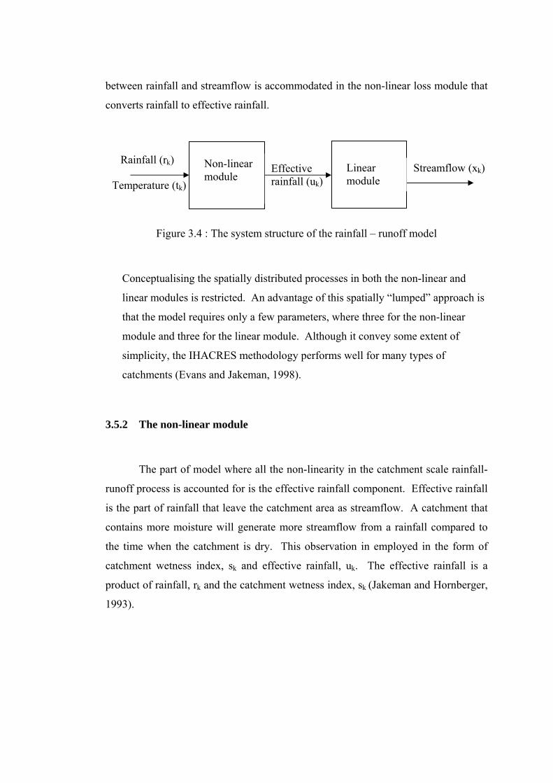
between rainfall and streamflow is accommodated in the non-linear loss module that

converts rainfall to effective rainfall.

Temperature (tk)

Rainfall (rk) Streamflow (xk) Effective rainfall (uk)

Linear module

Non-linear module

Figure 3.4 : The system structure of the rainfall – runoff model

Conceptualising the spatially distributed processes in both the non-linear and

linear modules is restricted. An advantage of this spatially “lumped” approach is

that the model requires only a few parameters, where three for the non-linear

module and three for the linear module. Although it convey some extent of

simplicity, the IHACRES methodology performs well for many types of

catchments (Evans and Jakeman, 1998).

3.5.2 The non-linear module

The part of model where all the non-linearity in the catchment scale rainfall-

runoff process is accounted for is the effective rainfall component. Effective rainfall

is the part of rainfall that leave the catchment area as streamflow. A catchment that

contains more moisture will generate more streamflow from a rainfall compared to

the time when the catchment is dry. This observation in employed in the form of

catchment wetness index, sk and effective rainfall, uk. The effective rainfall is a

product of rainfall, rk and the catchment wetness index, sk (Jakeman and Hornberger,

1993).

uk = rk sk [Eq. 3.3]

1)(

11 −⎟⎟⎠

⎞⎜⎜⎝

⎛−+= k

kwkk s

tCrs

τ, s0 = 0 [Eq. 3.4]

τw (tk) = τw e0.062f(R-tk), τw (tk) > 1 [Eq. 3.5] where uk is the effective rainfall

rk is the rainfall

sk is the catchment wetness index

C is the mass balance term

τw is the catchment drying rate at reference temperature

tk is the temperature

R is the reference temperature

f is the temperature dependence of drying rate

Parameter τw is the value of τw(tk) at a reference temperature chosen by the

user. In equation 3.4, τw(tk) controls the rate at which the catchment wetness index

decays in when there is no rainfall events. Parameter f controls the sensitivity of

τw(tk) to changes in temperature. For time intervals with rain, decay of catchment

wetness index still occurs but it is also incremented by a proportion mass balance

term of the rainfall. Value for parameter C is selected so that the volumes of

effective rainfall and observed streamflow over the model calibration period are

equal. This value is calculated automatically during the model calibration.

3.5.3 The linear module

In a simple discrete-time hydrograph, a unit of effective rainfall over one data

time step is considered to produce streamflow (b < 1) over the same time step. The

effective rainfall and flow is zero in the previous time step and effective rainfall is

zero in all following time steps. In each following time step, streamflow is a fixed

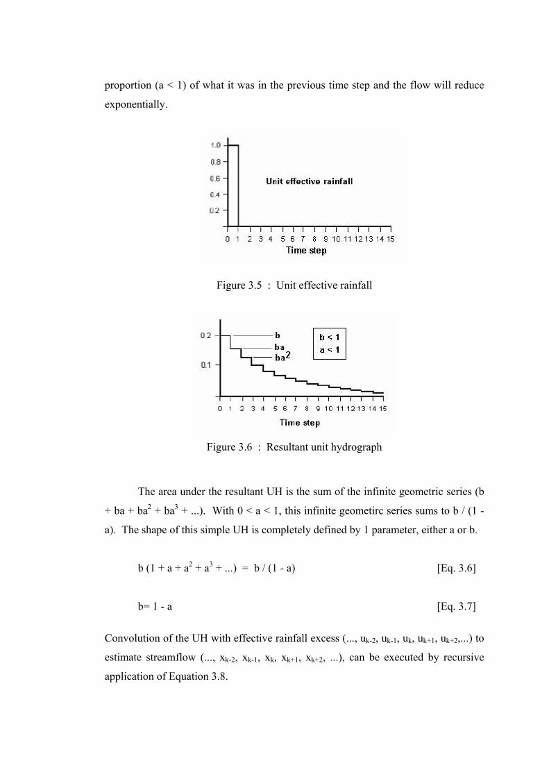
proportion (a < 1) of what it was in the previous time step and the flow will reduce

exponentially.

Figure 3.5 : Unit effective rainfall

Figure 3.6 : Resultant unit hydrograph

The area under the resultant UH is the sum of the infinite geometric series (b

+ ba + ba2 + ba3 + ...). With 0 < a < 1, this infinite geometirc series sums to b / (1 -

a). The shape of this simple UH is completely defined by 1 parameter, either a or b.

b (1 + a + a2 + a3 + ...) = b / (1 - a) [Eq. 3.6]

b= 1 - a [Eq. 3.7]

Convolution of the UH with effective rainfall excess (..., uk-2, uk-1, uk, uk+1, uk+2,...) to

estimate streamflow (..., xk-2, xk-1, xk, xk+1, xk+2, ...), can be executed by recursive

application of Equation 3.8.

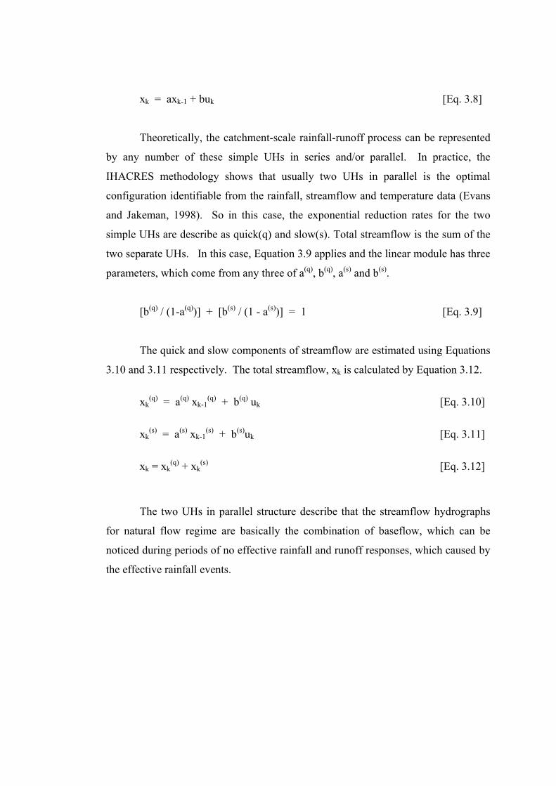
xk = axk-1 + buk [Eq. 3.8]

Theoretically, the catchment-scale rainfall-runoff process can be represented

by any number of these simple UHs in series and/or parallel. In practice, the

IHACRES methodology shows that usually two UHs in parallel is the optimal

configuration identifiable from the rainfall, streamflow and temperature data (Evans

and Jakeman, 1998). So in this case, the exponential reduction rates for the two

simple UHs are describe as quick(q) and slow(s). Total streamflow is the sum of the

two separate UHs. In this case, Equation 3.9 applies and the linear module has three

parameters, which come from any three of a(q), b(q), a(s) and b(s).

[b(q) / (1-a(q))] + [b(s) / (1 - a(s))] = 1 [Eq. 3.9]

The quick and slow components of streamflow are estimated using Equations

3.10 and 3.11 respectively. The total streamflow, xk is calculated by Equation 3.12.

xk

(q) = a(q) xk-1(q) + b(q) uk [Eq. 3.10]

xk

(s) = a(s) xk-1(s) + b(s)uk [Eq. 3.11]

xk = xk

(q) + xk(s) [Eq. 3.12]

The two UHs in parallel structure describe that the streamflow hydrographs

for natural flow regime are basically the combination of baseflow, which can be

noticed during periods of no effective rainfall and runoff responses, which caused by

the effective rainfall events.

3.5.4 Data requirement 3.5.4.1 Input data

IHACRES requires three sets of time series data as the input, which are:

• Observed rainfall (in mm or inches)

• Temperature (in degree Celsius, Fahrenheit, or Kelvin) or

evapotranspiration (in mm or inches)

• Observed streamflow (in m3/s, megalitres per time step, millimetres per time

step, l/s, or cubic feet per second).

The source of data must be in delimited ASCII text format. Each time series

of the required data can be stored in one file with three separate columns for each

type of data or in three different files for each data.

The timesteps of the time series supported are in minutes, hours and days.

Catchment area in km2 may be required depend on the measurements units used for

the observed streamflow data.

3.5.4.2 Calculated data

After the simulation, a time series of modelled streamflow will be produced,

along with multiple statistics which describe the characteristics of each series.

Almost all of the data and tables can be exported as comma delimited ASCII text

files. Graphs are also viewable in the program.

The results of the grid searches done during calibration can be saved as .igs

files which can later be reopen for reuse. After the data has been loaded and a

project is created, the project file can be saved as a project (.ipr) file.

3.5.5 The three modes of operation

3.5.5.1 Data

Each component has its own sets of tabs to serve as its own function. The

data component has three tabs which are:

• Summary - a summary of that data that is loaded

• Import - a tool to load the time series data as input

• View - a tool to review the loaded data in graph form

3.5.5.2 Calibration of a model

The calibration mode has two tabs which are:

• Model - to build the model by both linear and non-linear modules

• Periods - to define the calibration periods

The calibration period will have to be set first before the calibration of the

model can be executed to obtain the parameter sets.

3.5.5.3 Simulation

Simulation cannot be run before the calibration process is completed. After

the calibration process, simulation is run to obtain the modelled streamflow time

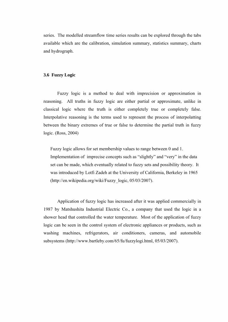
series. The modelled streamflow time series results can be explored through the tabs

available which are the calibration, simulation summary, statistics summary, charts

and hydrograph.

3.6 Fuzzy Logic

Fuzzy logic is a method to deal with imprecision or approximation in

reasoning. All truths in fuzzy logic are either partial or approximate, unlike in

classical logic where the truth is either completely true or completely false.

Interpolative reasoning is the terms used to represent the process of interpolatting

between the binary extremes of true or false to determine the partial truth in fuzzy

logic. (Ross, 2004)

Fuzzy logic allows for set membership values to range between 0 and 1.

Implementation of imprecise concepts such as “slightly” and “very” in the data

set can be made, which eventually related to fuzzy sets and possibility theory. It

was introduced by Lotfi Zadeh at the University of California, Berkeley in 1965

(http://en.wikipedia.org/wiki/Fuzzy_logic, 05/03/2007).

Application of fuzzy logic has increased after it was applied commercially in

1987 by Matshushita Industrial Electric Co., a company that used the logic in a

shower head that controlled the water temperature. Most of the application of fuzzy

logic can be seen in the control system of electronic appliances or products, such as

washing machines, refrigerators, air conditioners, cameras, and automobile

subsystems (http://www.bartleby.com/65/fu/fuzzylogi.html, 05/03/2007).

3.6.1 Fuzzy membership function

Decisions making in processes that contain certain degree of uncertainty has

been shown to be less than perfect. Set membership is the key to decision making

when faced with uncertainty (Ross, 2004). All information contained in a fuzzy set

can be described by its membership function. The membership of an element may be

measured by a degree, which also known as the membership degree of that element

to the set. The value will range within the interval of [0,1] by agreement (Galindo et

al., 2006).

The region in the universe of a typical fuzzy set consists of the core, support

and boudaries. The core of a membership function is the region of the universe that

is characterized by complete and full membership in the set. The core is made out of

the element x of the universe, µ so that µ(x) = 1. The support of a membership

function is the region of the universe that is characterised by nonzero membership in

the set. The support made of other elements x of the universe so that µ(x) > 0.

The boundaries of a membership function is the region of the universe which

contain elements that have a nonzero membership but not complete membership.

The boundaries comprise those elements x of the universe such that 0 < µ(x) <1.

These elements of the universe are those with some degree of fuzziness, or only

partial membership in the fuzzy set.

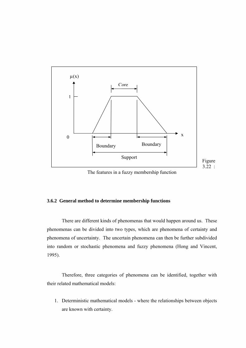
µ(x)

Core

1 x 0 Boundary Boundary Support Figure 3.22 :

The features in a fuzzy membership function 3.6.2 General method to determine membership functions

There are different kinds of phenomenas that would happen around us. These

phenomenas can be divided into two types, which are phenomena of certainty and

phenomena of uncertainty. The uncertain phenomena can then be further subdivided

into random or stochastic phenomena and fuzzy phenomena (Hong and Vincent,

1995).

Therefore, three categories of phenomena can be identified, together with

their related mathematical models:

1. Deterministic mathematical models - where the relationships between objects

are known with certainty.

2. Random (stochastic) mathematical models - where the relationships between

objects are uncertain or random in nature.

3. Fuzzy mathematical models - where objects and relationships between

objects are fuzzy.

The main difference between random phenomena and fuzzy phenomena is

that the random events have well-defined meaning, while fuzzy concept does not

have a precise extension because it is hard to judge whether an object belongs to the

concept. Randomness is a deficiency of the law of probability and that fuzziness is a

deficiency of the law of the excluded middle. Probability theory applies the random

concept to generalized laws of probability. Fuzzy set theory applies the fuzzy

property to the generalized law of the excluded middle, which is the law of

membership from fuzziness (Hong and Vincent, 1995).

Probability reflects the internal relations and interactions of events under

certain conditions. It could be very objective if a stable frequency is available from

repeated experiments. Similarly, a stable frequency results from fuzzy statistical

tests and can serve as the degree of membership in the objective sense. In many

cases, the degree of membership can be determined by fuzzy statistical methods.

A random experiment has four basic requirements:

1. A sample space Ω that is formed by all related factors.

2. An event A that is a fixed and crisp subset of Ω.

3. A variable ω that is in Ω; once ω is determined, so are all the factors on their

stated spaces.

4. A condition S that serve as restrictions on variable ω.

Figure 3.23 : A random experiment (A is fixed but ω varies)

The basic reason for randomness to exist is that the condition S is unable to

restrict ω to a fixed point. Moreover, if S Φ≠∩ A and A, then Φ≠∩ cAS

AS ∩∈ω shows that the event A has occurred; otherwise it has not. That means A

is a random event under the condition S. On random experiments, the following

observations can be made:

1. The purpose of a random experiment is to study the uncertainty with certain

or deterministic procedures.

2. A fundamental requirement of a random experiment is to clearly tell whether

an event A has occurred or not.

3. A special characteristic of random experiment is that A is fixed, while ω is

not.

4. After n times of repeated experiments, the frequency of A can be computed

by Equation 3.13.

Frequency of A = The number of trials when ω ∈ A [Eq. 3.13]

n

It is well known that as n becomes very large, the above frequency tends to

stabilize or converge to a fixed number. This number is called the probability of A

under S.

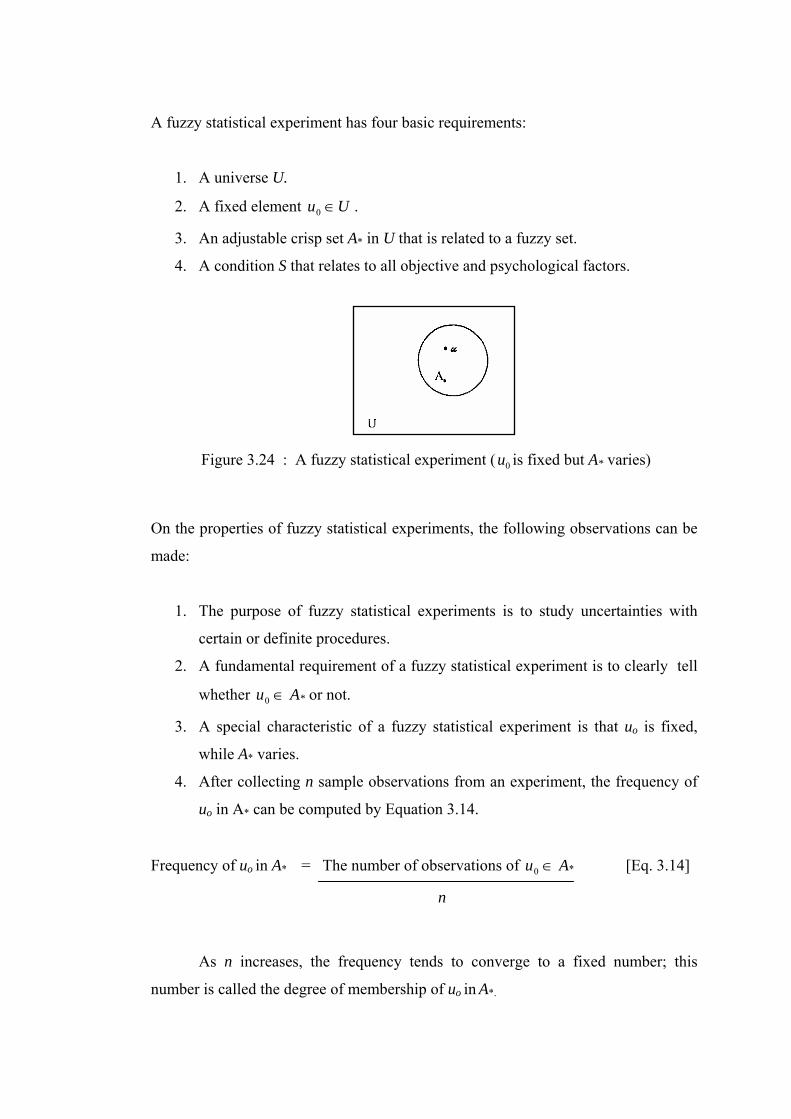
A fuzzy statistical experiment has four basic requirements:

1. A universe U.

2. A fixed element . Uu ∈0

3. An adjustable crisp set A* in U that is related to a fuzzy set.

4. A condition S that relates to all objective and psychological factors.

Figure 3.24 : A fuzzy statistical experiment ( is fixed but A0u * varies)

On the properties of fuzzy statistical experiments, the following observations can be

made:

1. The purpose of fuzzy statistical experiments is to study uncertainties with

certain or definite procedures.

2. A fundamental requirement of a fuzzy statistical experiment is to clearly tell

whether A∈0u * or not.

3. A special characteristic of a fuzzy statistical experiment is that uo is fixed,

while A* varies.

4. After collecting n sample observations from an experiment, the frequency of

uo in A* can be computed by Equation 3.14.

Frequency of uo in A* = The number of observations of ∈0u A* [Eq. 3.14]

n

As n increases, the frequency tends to converge to a fixed number; this

number is called the degree of membership of uo in A*.

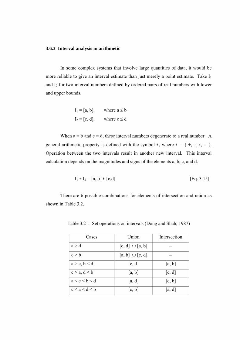
3.6.3 Interval analysis in arithmetic

In some complex systems that involve large quantities of data, it would be

more reliable to give an interval estimate than just merely a point estimate. Take I1

and I2 for two interval numbers defined by ordered pairs of real numbers with lower

and upper bounds.

I1 = [a, b], where a ≤ b

I2 = [c, d], where c ≤ d

When a = b and c = d, these interval numbers degenerate to a real number. A

general arithmetic property is defined with the symbol ∗, where ∗ = +, -, x, ÷ .

Operation between the two intervals result in another new interval. This interval

calculation depends on the magnitudes and signs of the elements a, b, c, and d.

I1 ∗ I2 = [a, b] ∗ [c,d] [Eq. 3.15]

There are 6 possible combinations for elements of intersection and union as

shown in Table 3.2.

Table 3.2 : Set operations on intervals (Dong and Shah, 1987)

Cases Union Intersection

a > d [c, d] ∪ [a, b] ¬

c > b [a, b] ∪ [c, d] ¬

a > c, b < d [c, d] [a, b]

c > a, d < b [a, b] [c, d]

a < c < b < d [a, d] [c, b]

c < a < d < b [c, b] [a, d]

Based on the information in Table 3.2, the four arithmetic operations

associated with Equation 3.15 are given as follows:

[a,b] + [c,d] = [a + c, b + d] [Eq. 3.16]

[a,b] - [c,d] = [a + c, b + d] [Eq. 3.17]

[a,b] • [c,d] = [min (ac, ad, bc, bd), max (ac, ad, bc, bd)] [Eq. 3.18]

[a,b] / [c,d] = [a,b] • ⎥⎦⎤

⎢⎣⎡

cd1,1 , if 0 ∉ [c,d] [Eq. 3.19]

Interval arithmetic follows properties of associativity and commutativity for

both summations and products, but it does not follow the property of distributivity.

Rather, intervals do follow a special subclass of distributivity known as

subdistributivity. Assume that I, J and K are interval numbers;

Associativity:

I + (J + K) = (I + J) + K [Eq. 3.20]

I • (J • K) = (I • J) • K [Eq. 3.21]

Commutativity:

I + J = J + I [Eq. 3.22]

I • J = J • I [Eq. 3.23]

Subdistributivity:

I • (J + K) ⊂ I • J + I • K [Eq. 3.24]

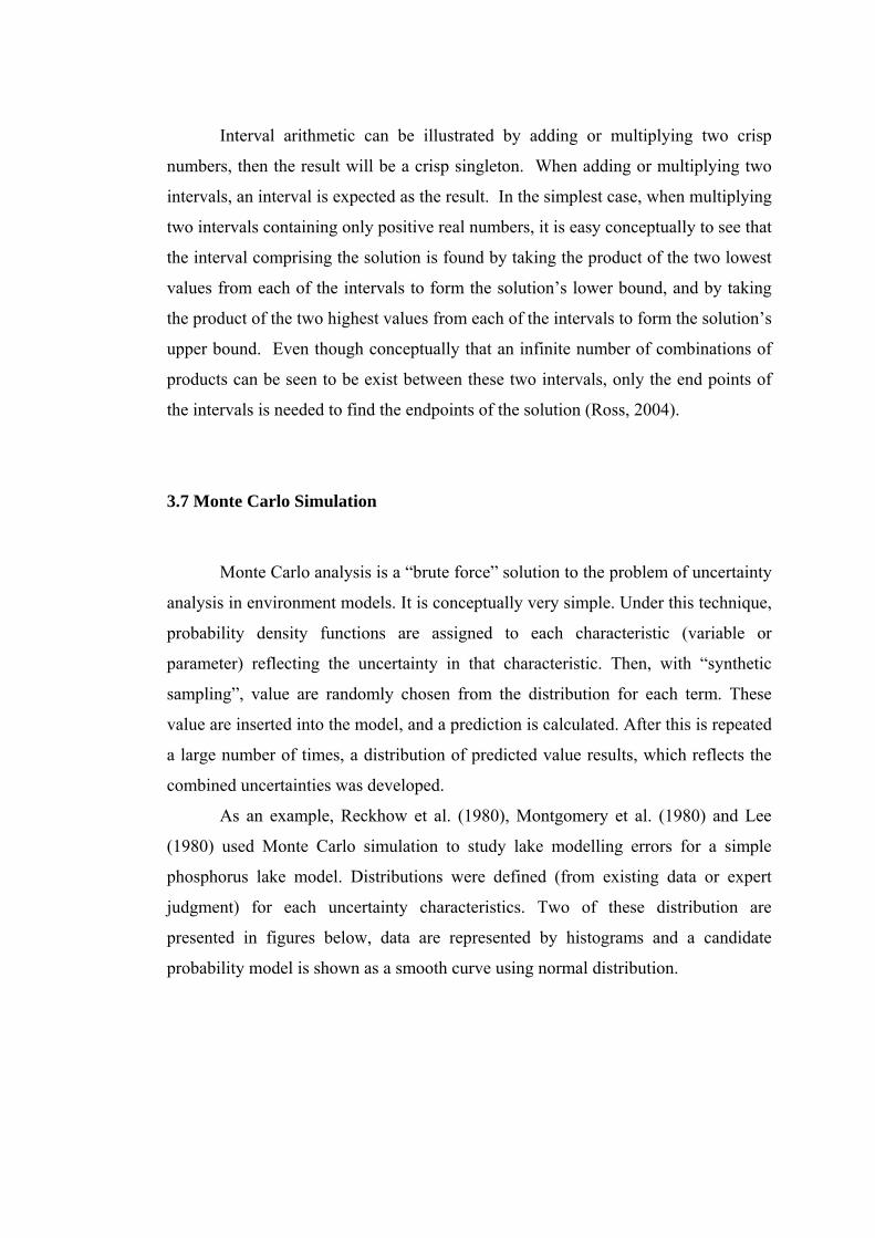
Interval arithmetic can be illustrated by adding or multiplying two crisp

numbers, then the result will be a crisp singleton. When adding or multiplying two

intervals, an interval is expected as the result. In the simplest case, when multiplying

two intervals containing only positive real numbers, it is easy conceptually to see that

the interval comprising the solution is found by taking the product of the two lowest

values from each of the intervals to form the solution’s lower bound, and by taking

the product of the two highest values from each of the intervals to form the solution’s

upper bound. Even though conceptually that an infinite number of combinations of

products can be seen to be exist between these two intervals, only the end points of

the intervals is needed to find the endpoints of the solution (Ross, 2004).

3.7 Monte Carlo Simulation

Monte Carlo analysis is a “brute force” solution to the problem of uncertainty

analysis in environment models. It is conceptually very simple. Under this technique,

probability density functions are assigned to each characteristic (variable or

parameter) reflecting the uncertainty in that characteristic. Then, with “synthetic

sampling”, value are randomly chosen from the distribution for each term. These

value are inserted into the model, and a prediction is calculated. After this is repeated

a large number of times, a distribution of predicted value results, which reflects the

combined uncertainties was developed.

As an example, Reckhow et al. (1980), Montgomery et al. (1980) and Lee

(1980) used Monte Carlo simulation to study lake modelling errors for a simple

phosphorus lake model. Distributions were defined (from existing data or expert

judgment) for each uncertainty characteristics. Two of these distribution are

presented in figures below, data are represented by histograms and a candidate

probability model is shown as a smooth curve using normal distribution.

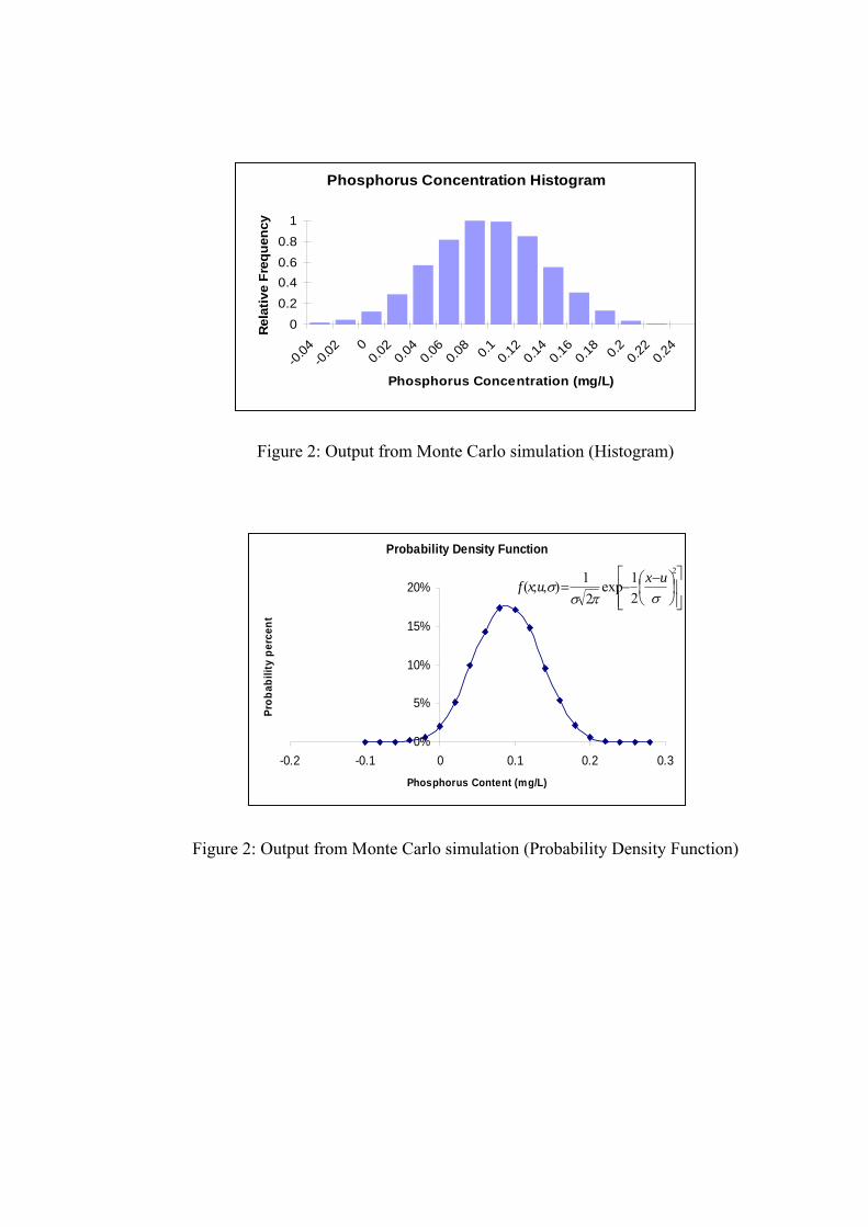
Phosphorus Concentration Histogram

00.20.40.60.8

1

-0.04

-0.02 0

0.02

0.04

0.06

0.08 0.1 0.1

20.1

40.1

60.1

8 0.2 0.22

0.24

Phosphorus Concentration (mg/L)

Rel

ativ

e Fr

eque

ncy

Figure 2: Output from Monte Carlo simulation (Histogram)

Probability Density Function

0%

5%

10%

15%

20%

-0.2 -0.1 0 0.1 0.2 0.3Phosphorus Content (mg/L)

Prob

abili

ty p

erce

nt

⎥⎥⎦

⎤

⎢⎢⎣

⎡⎟⎠⎞

⎜⎝⎛ −

−=2

21exp

21),;(

σπσσ uxuxf

Figure 2: Output from Monte Carlo simulation (Probability Density Function)

CHAPTER 4

DATA ANALYSIS AND DISCUSSIONS 4.1 Data collection There are four main type of data that need to be obtained in this study. The

data were collected either by site investigations, sampling and testing, previous

records or calculations. Some raw data will have to be analysed before it could be

used. Later, the precipition, temperature and observed streamflow data will become

the input to the IHACRES model to predict of streamflow for the catchment. The

phophorus content and the modelled streamflow will be generated using fuzzy

membership function with interval numbers operation for Vollenweider model.

4.2 Phosphorus content

Ten water samples were taken in each site visit from the ten stations within

the catchment area. The water samples were brought back and tested at the

laboratory to obtain the phosphorus content of the water samples. The same stations

that were determined in the first visit were used for the second and third visits. There

are some data that were unable to obtain in the second visit, which was caused by

inaccessibility to the station area due to high water level that damaged the access

roads.

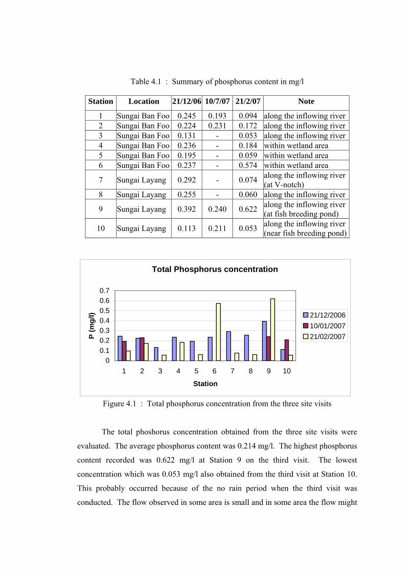
Table 4.1 : Summary of phosphorus content in mg/l

Station Location 21/12/06 10/7/07 21/2/07 Note

1 Sungai Ban Foo 0.245 0.193 0.094 along the inflowing river2 Sungai Ban Foo 0.224 0.231 0.172 along the inflowing river3 Sungai Ban Foo 0.131 - 0.053 along the inflowing river4 Sungai Ban Foo 0.236 - 0.184 within wetland area 5 Sungai Ban Foo 0.195 - 0.059 within wetland area 6 Sungai Ban Foo 0.237 - 0.574 within wetland area

7 Sungai Layang 0.292 - 0.074 along the inflowing river(at V-notch)

8 Sungai Layang 0.255 - 0.060 along the inflowing river

9 Sungai Layang 0.392 0.240 0.622 along the inflowing river(at fish breeding pond)

10 Sungai Layang 0.113 0.211 0.053 along the inflowing river(near fish breeding pond)

Total Phosphorus concentration

00.10.20.30.40.50.60.7

1 2 3 4 5 6 7 8 9 10

Station

P (m

g/l) 21/12/2006

10/01/200721/02/2007

Figure 4.1 : Total phosphorus concentration from the three site visits

The total phoshorus concentration obtained from the three site visits were

evaluated. The average phosphorus content was 0.214 mg/l. The highest phosphorus

content recorded was 0.622 mg/l at Station 9 on the third visit. The lowest

concentration which was 0.053 mg/l also obtained from the third visit at Station 10.

This probably occurred because of the no rain period when the third visit was

conducted. The flow observed in some area is small and in some area the flow might

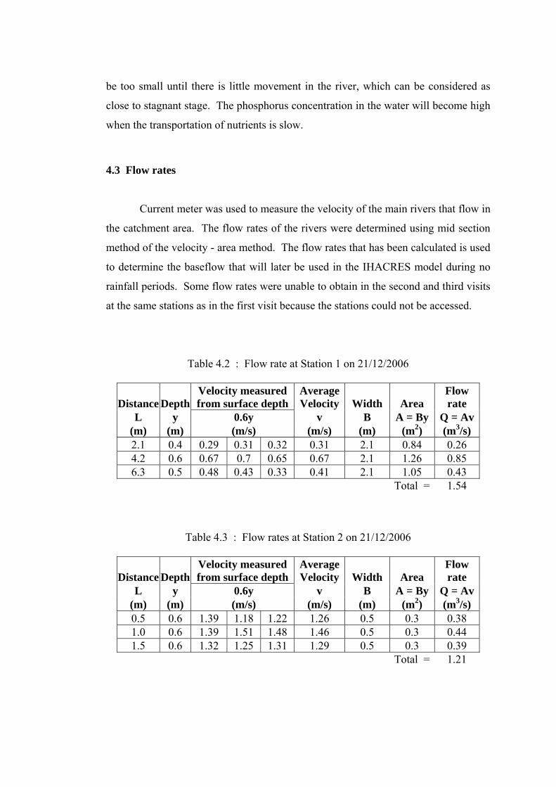
be too small until there is little movement in the river, which can be considered as

close to stagnant stage. The phosphorus concentration in the water will become high

when the transportation of nutrients is slow.

4.3 Flow rates Current meter was used to measure the velocity of the main rivers that flow in

the catchment area. The flow rates of the rivers were determined using mid section

method of the velocity - area method. The flow rates that has been calculated is used

to determine the baseflow that will later be used in the IHACRES model during no

rainfall periods. Some flow rates were unable to obtain in the second and third visits

at the same stations as in the first visit because the stations could not be accessed.

Table 4.2 : Flow rate at Station 1 on 21/12/2006

Distance Depth Velocity measured from surface depth

Average Velocity Width Area

Flow rate

L y 0.6y v B A = By Q = Av(m) (m) (m/s) (m/s) (m) (m2) (m3/s) 2.1 0.4 0.29 0.31 0.32 0.31 2.1 0.84 0.26 4.2 0.6 0.67 0.7 0.65 0.67 2.1 1.26 0.85 6.3 0.5 0.48 0.43 0.33 0.41 2.1 1.05 0.43

Total = 1.54

Table 4.3 : Flow rates at Station 2 on 21/12/2006

Distance Depth Velocity measured from surface depth

Average Velocity Width Area

Flow rate

L y 0.6y v B A = By Q = Av(m) (m) (m/s) (m/s) (m) (m2) (m3/s) 0.5 0.6 1.39 1.18 1.22 1.26 0.5 0.3 0.38 1.0 0.6 1.39 1.51 1.48 1.46 0.5 0.3 0.44 1.5 0.6 1.32 1.25 1.31 1.29 0.5 0.3 0.39

Total = 1.21

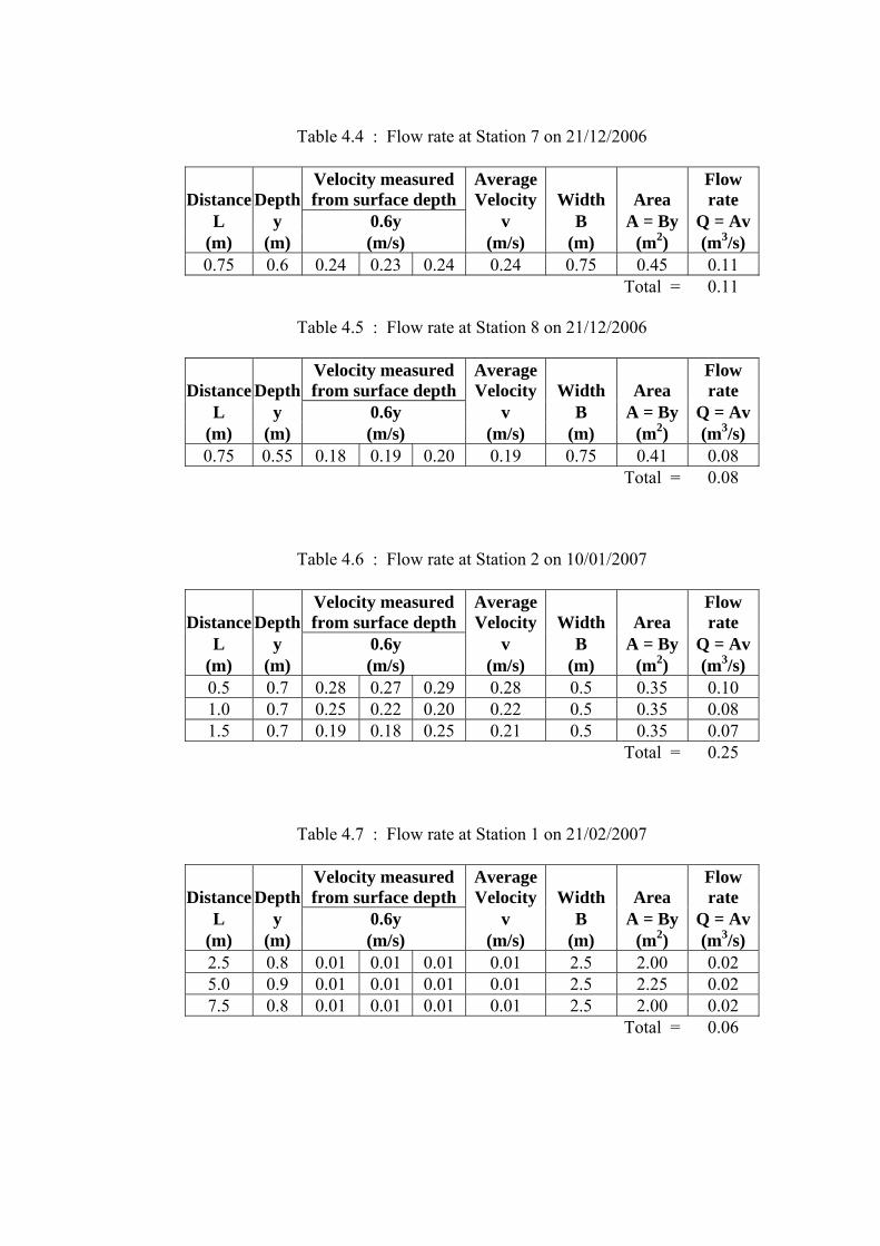
Table 4.4 : Flow rate at Station 7 on 21/12/2006

Distance Depth Velocity measured from surface depth

Average Velocity Width Area

Flow rate

L y 0.6y v B A = By Q = Av(m) (m) (m/s) (m/s) (m) (m2) (m3/s) 0.75 0.6 0.24 0.23 0.24 0.24 0.75 0.45 0.11

Total = 0.11

Table 4.5 : Flow rate at Station 8 on 21/12/2006

Distance Depth Velocity measured from surface depth

Average Velocity Width Area

Flow rate

L y 0.6y v B A = By Q = Av(m) (m) (m/s) (m/s) (m) (m2) (m3/s) 0.75 0.55 0.18 0.19 0.20 0.19 0.75 0.41 0.08

Total = 0.08

Table 4.6 : Flow rate at Station 2 on 10/01/2007

Distance Depth Velocity measured from surface depth

Average Velocity Width Area

Flow rate

L y 0.6y v B A = By Q = Av(m) (m) (m/s) (m/s) (m) (m2) (m3/s) 0.5 0.7 0.28 0.27 0.29 0.28 0.5 0.35 0.10 1.0 0.7 0.25 0.22 0.20 0.22 0.5 0.35 0.08 1.5 0.7 0.19 0.18 0.25 0.21 0.5 0.35 0.07

Total = 0.25

Table 4.7 : Flow rate at Station 1 on 21/02/2007

Distance Depth Velocity measured from surface depth

Average Velocity Width Area

Flow rate

L y 0.6y v B A = By Q = Av(m) (m) (m/s) (m/s) (m) (m2) (m3/s) 2.5 0.8 0.01 0.01 0.01 0.01 2.5 2.00 0.02 5.0 0.9 0.01 0.01 0.01 0.01 2.5 2.25 0.02 7.5 0.8 0.01 0.01 0.01 0.01 2.5 2.00 0.02

Total = 0.06

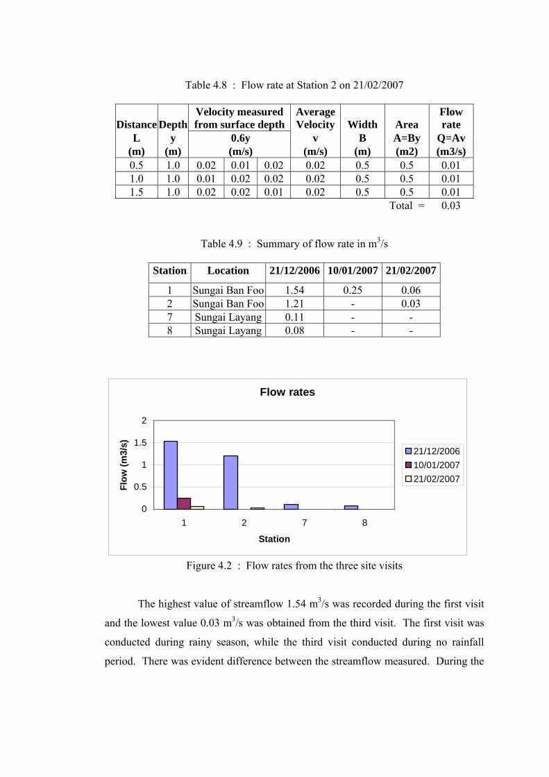
Table 4.8 : Flow rate at Station 2 on 21/02/2007

Distance Depth Velocity measured from surface depth

Average Velocity Width Area

Flow rate

L y 0.6y v B A=By Q=Av (m) (m) (m/s) (m/s) (m) (m2) (m3/s) 0.5 1.0 0.02 0.01 0.02 0.02 0.5 0.5 0.01 1.0 1.0 0.01 0.02 0.02 0.02 0.5 0.5 0.01 1.5 1.0 0.02 0.02 0.01 0.02 0.5 0.5 0.01

Total = 0.03

Table 4.9 : Summary of flow rate in m3/s

Station Location 21/12/2006 10/01/2007 21/02/2007

1 Sungai Ban Foo 1.54 0.25 0.06 2 Sungai Ban Foo 1.21 - 0.03 7 Sungai Layang 0.11 - - 8 Sungai Layang 0.08 - -

Flow rates

0

0.5

1

1.5

2

1 2 7 8

Station

Flow

(m3/

s)

21/12/200610/01/200721/02/2007

Figure 4.2 : Flow rates from the three site visits

The highest value of streamflow 1.54 m3/s was recorded during the first visit

and the lowest value 0.03 m3/s was obtained from the third visit. The first visit was

conducted during rainy season, while the third visit conducted during no rainfall

period. There was evident difference between the streamflow measured. During the

first visit, the flow of the river is observed to be high. Meanwhile, the observation

result from the third visit was that there was only small flow in the river.

4.4 Temperature Daily temperature data were obtained as an input for the IHACRES model.

The data was obtain from the Malaysian Meteorological Department. The station for

the temperature measurement is located at Senai with the station number 48679. It is

37.8 m above mean sea level and situated in the coordinates of latitudes 1o 38’ N and

longitudes 103o 40’ E.

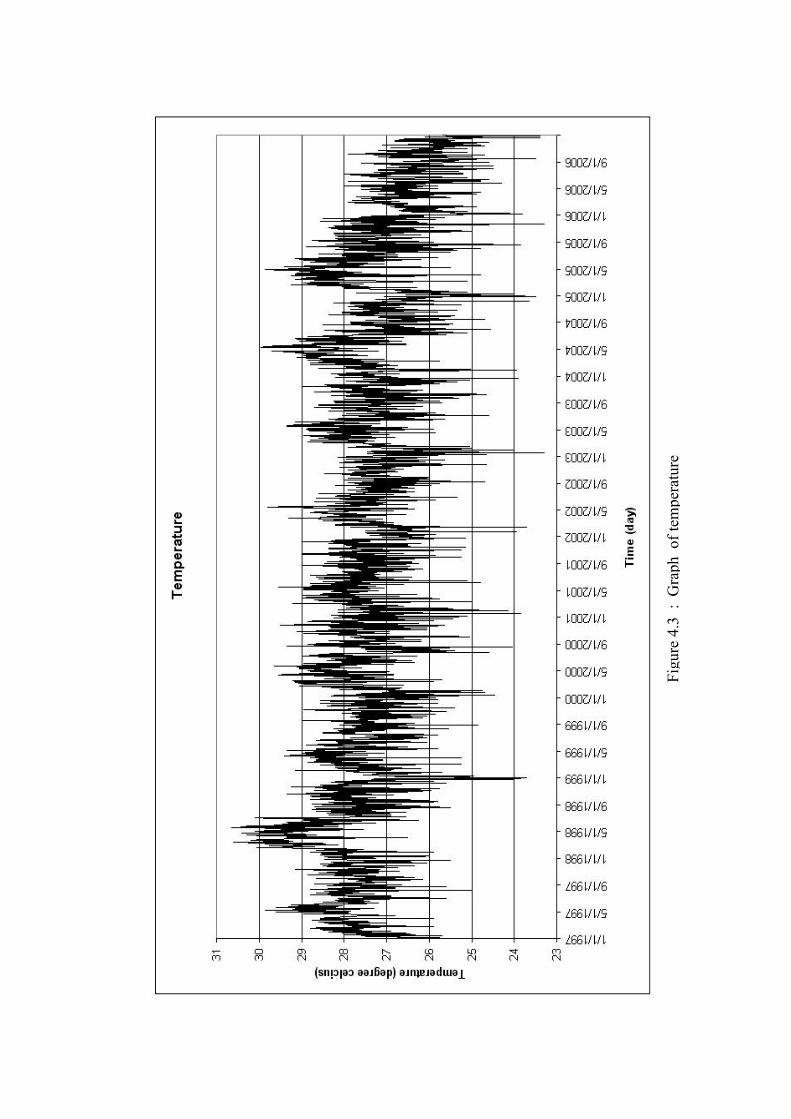
Figu

re 4

.3 :

Gra

ph o

f tem

pera

ture

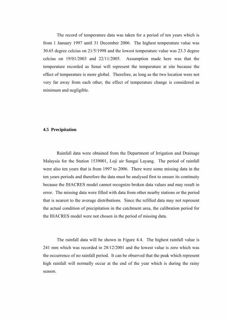
The record of temperature data was taken for a period of ten years which is

from 1 January 1997 until 31 December 2006. The highest temperature value was

30.65 degree celcius on 21/5/1998 and the lowest temperature value was 23.3 degree

celcius on 19/01/2003 and 22/11/2005. Assumption made here was that the

temperature recorded as Senai will represent the temperature at site because the

effect of temperature is more global. Therefore, as long as the two location were not

very far away from each other, the effect of temperature change is considered as

minimum and negligible.

4.5 Precipitation

Rainfall data were obtained from the Department of Irrigation and Drainage

Malaysia for the Station 1539001, Loji air Sungai Layang. The period of rainfall

were also ten years that is from 1997 to 2006. There were some missing data in the

ten years periods and therefore the data must be analysed first to ensure its continuity

because the IHACRES model cannot recognize broken data values and may result in

error. The missing data were filled with data from other nearby stations or the period

that is nearest to the average distributions. Since the refilled data may not represent

the actual condition of precipitation in the catchment area, the calibration period for

the IHACRES model were not chosen in the period of missing data.

The rainfall data will be shown in Figure 4.4. The highest rainfall value is

241 mm which was recorded in 28/12/2001 and the lowest value is zero which was

the occurrence of no rainfall period. It can be observed that the peak which represent

high rainfall will normally occur at the end of the year which is during the rainy

season.

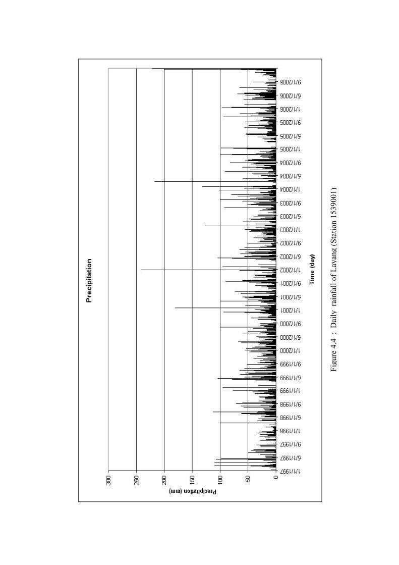
Figu

re 4

.4 :

Dai

ly r

ainf

all o

f Lay

ang

(Sta

tion

1539

001)

4.6 Evaporation Evaporation data is used for runoff analysis of the catchment, which is also

regard as the observed streamflow. Daily evaporation data for Station 1539301 were

obtained from the Department of Irrigation and Drainage Malaysia with the same

period as the rainfall. There also exist some missing data and the missing data were

filled with data from other nearby stations or the period that is nearest to the average

distributions.

The evaporation data will be shown in Figure 4.5. The highest evaporation is

12 mm which was recorded in 9/1/2003 and the lowest is zero which indicates that

no evaporation occurs during the period.

4.7 Infiltration

Infiltration data will have to be calculated for the use in the storage equation

in runoff analysis later. The Horton model is used for the calculation of infiltration

values. The parameter used are based on Table 14.4 from the MASMA manual. The

soil at the research area can be classified as loam soil which consists of sand, clay

and silt in approximately equal proportions (Faradilah, 2006).

Infiltration Rate, ( ) Ktcoc efffF −−+= [Eq. 4.1]

where fo = Initial infiltration rate

= 75 mm / hr

fc = Final infiltration rate

= 5.65 mm / hr

t = time (hr)

K = Coefficient ( 4 hr)

Figu

re 4

.5 :

Dai

ly e

vapo

ratio

n of

Lay

ang

(Sta

tion

1539

301)

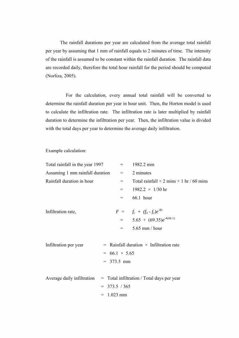
The rainfall durations per year are calculated from the average total rainfall

per year by assuming that 1 mm of rainfall equals to 2 minutes of time. The intensity

of the rainfall is assumed to be constant within the rainfall duration. The rainfall data

are recorded daily, therefore the total hour rainfall for the period should be computed

(Norliza, 2005).

For the calculation, every annual total rainfall will be converted to

determine the rainfall duration per year in hour unit. Then, the Horton model is used

to calculate the infiltration rate. The infiltration rate is later multiplied by rainfall

duration to determine the infiltration per year. Then, the infiltration value is divided

with the total days per year to determine the average daily infiltration.

Example calculation:

Total rainfall in the year 1997 = 1982.2 mm

Assuming 1 mm rainfall duration = 2 minutes

Rainfall duration in hour = Total rainfall × 2 mins × 1 hr / 60 mins

= 1982.2 × 1/30 hr

= 66.1 hour

Infiltration rate, F = fc + (fo - fc)e-Kt

= 5.65 + (69.35)e-4(66.1)

= 5.65 mm / hour

Infiltration per year = Rainfall duration × Infiltration rate

= 66.1 × 5.65

= 373.5 mm

Average daily infiltration = Total infiltration / Total days per year

= 373.5 / 365

= 1.023 mm

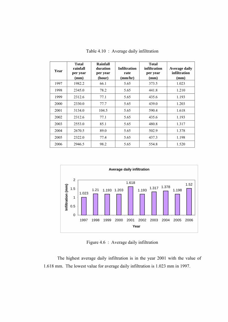
Table 4.10 : Average daily infiltration

Total

rainfall per year

Rainfall duration per year

Infiltration rate

Total infiltration

per year Average daily

infiltration Year

(mm) (hour) (mm/hr) (mm) (mm) 1997 1982.2 66.1 5.65 373.5 1.023

1998 2345.0 78.2 5.65 441.8 1.210

1999 2312.6 77.1 5.65 435.6 1.193

2000 2330.0 77.7 5.65 439.0 1.203

2001 3134.0 104.5 5.65 590.4 1.618

2002 2312.6 77.1 5.65 435.6 1.193

2003 2553.0 85.1 5.65 480.8 1.317

2004 2670.5 89.0 5.65 502.9 1.378

2005 2322.0 77.4 5.65 437.3 1.198

2006 2946.5 98.2 5.65 554.8 1.520

Average daily infiltration

1.0231.21 1.193 1.203

1.618

1.193 1.317 1.3781.198

1.52

0

0.5

1

1.5

2

1997 1998 1999 2000 2001 2002 2003 2004 2005 2006

Year

Infil

trat

ion

(mm

)

Figure 4.6 : Average daily infiltration The highest average daily infiltration is in the year 2001 with the value of

1.618 mm. The lowest value for average daily infiltration is 1.023 mm in 1997.

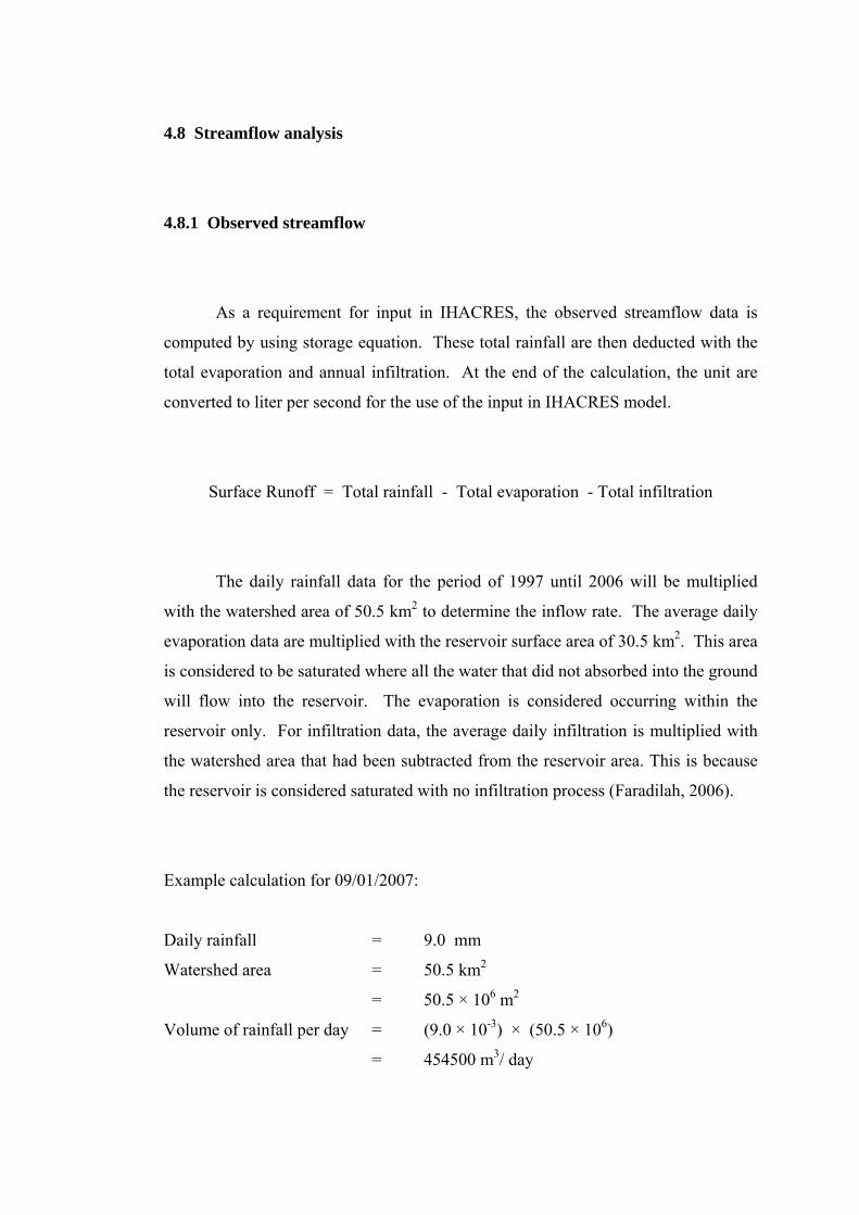
4.8 Streamflow analysis

4.8.1 Observed streamflow

As a requirement for input in IHACRES, the observed streamflow data is

computed by using storage equation. These total rainfall are then deducted with the

total evaporation and annual infiltration. At the end of the calculation, the unit are

converted to liter per second for the use of the input in IHACRES model.

Surface Runoff = Total rainfall - Total evaporation - Total infiltration

The daily rainfall data for the period of 1997 until 2006 will be multiplied

with the watershed area of 50.5 km2 to determine the inflow rate. The average daily

evaporation data are multiplied with the reservoir surface area of 30.5 km2. This area

is considered to be saturated where all the water that did not absorbed into the ground

will flow into the reservoir. The evaporation is considered occurring within the

reservoir only. For infiltration data, the average daily infiltration is multiplied with

the watershed area that had been subtracted from the reservoir area. This is because

the reservoir is considered saturated with no infiltration process (Faradilah, 2006).

Example calculation for 09/01/2007:

Daily rainfall = 9.0 mm

Watershed area = 50.5 km2

= 50.5 × 106 m2

Volume of rainfall per day = (9.0 × 10-3) × (50.5 × 106)

= 454500 m3/ day

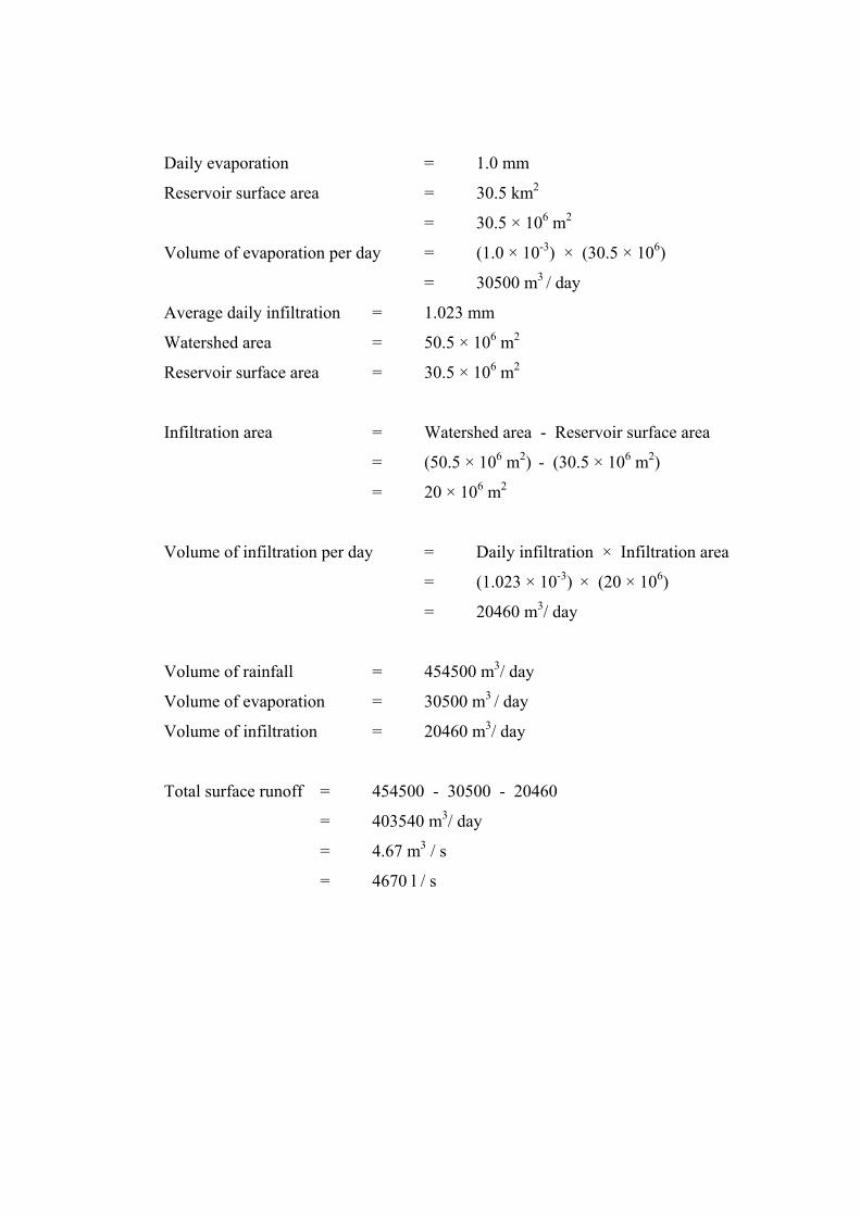
Daily evaporation = 1.0 mm

Reservoir surface area = 30.5 km2

= 30.5 × 106 m2

Volume of evaporation per day = (1.0 × 10-3) × (30.5 × 106)

= 30500 m3 / day

Average daily infiltration = 1.023 mm

Watershed area = 50.5 × 106 m2

Reservoir surface area = 30.5 × 106 m2

Infiltration area = Watershed area - Reservoir surface area

= (50.5 × 106 m2) - (30.5 × 106 m2)

= 20 × 106 m2

Volume of infiltration per day = Daily infiltration × Infiltration area

= (1.023 × 10-3) × (20 × 106)

= 20460 m3/ day

Volume of rainfall = 454500 m3/ day

Volume of evaporation = 30500 m3 / day

Volume of infiltration = 20460 m3/ day

Total surface runoff = 454500 - 30500 - 20460

= 403540 m3/ day

= 4.67 m3 / s

= 4670 l / s

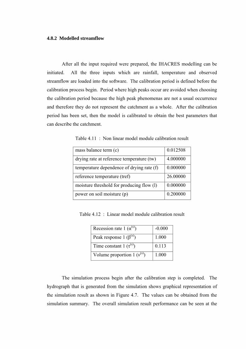
4.8.2 Modelled streamflow

After all the input required were prepared, the IHACRES modelling can be

initiated. All the three inputs which are rainfall, temperature and observed

streamflow are loaded into the software. The calibration period is defined before the

calibration process begin. Period where high peaks occur are avoided when choosing

the calibration period because the high peak phenomenas are not a usual occurrence

and therefore they do not represent the catchment as a whole. After the calibration

period has been set, then the model is calibrated to obtain the best parameters that

can describe the catchment.

Table 4.11 : Non linear model module calibration result

mass balance term (c) 0.012508

drying rate at reference temperature (tw) 4.000000

temperature dependence of drying rate (f) 0.000000

reference temperature (tref) 26.00000

moisture threshold for producing flow (l) 0.000000

power on soil moisture (p) 0.200000

Table 4.12 : Linear model module calibration result

Recession rate 1 (α(s)) -0.000

Peak response 1 (β(s)) 1.000

Time constant 1 (τ(s)) 0.113

Volume proportion 1 (v(s)) 1.000

The simulation process begin after the calibration step is completed. The

hydrograph that is generated from the simulation shows graphical representation of

the simulation result as shown in Figure 4.7. The values can be obtained from the

simulation summary. The overall simulation result performance can be seen at the

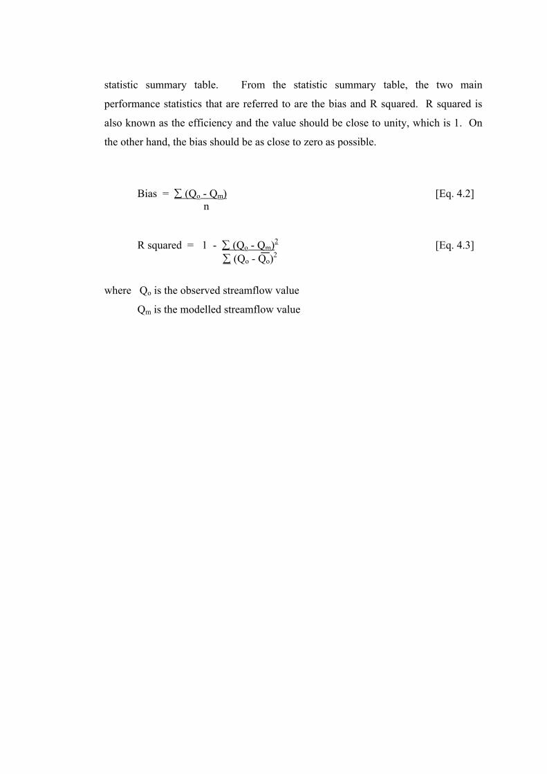
statistic summary table. From the statistic summary table, the two main

performance statistics that are referred to are the bias and R squared. R squared is

also known as the efficiency and the value should be close to unity, which is 1. On

the other hand, the bias should be as close to zero as possible.

Bias = ∑ (Qo - Qm) [Eq. 4.2]

n

R squared = 1 - ∑ (Qo - Qm)2 [Eq. 4.3] ∑ (Qo - Qo)2

where Qo is the observed streamflow value

Qm is the modelled streamflow value

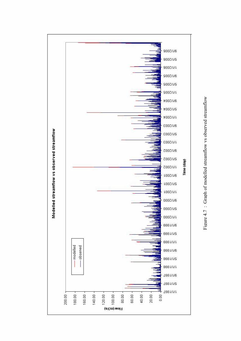
Figu

re 4

.7 :

Gra

ph o

f mod

elle

d st

ream

flow

vs o

bser

ved

stre

amflo

w

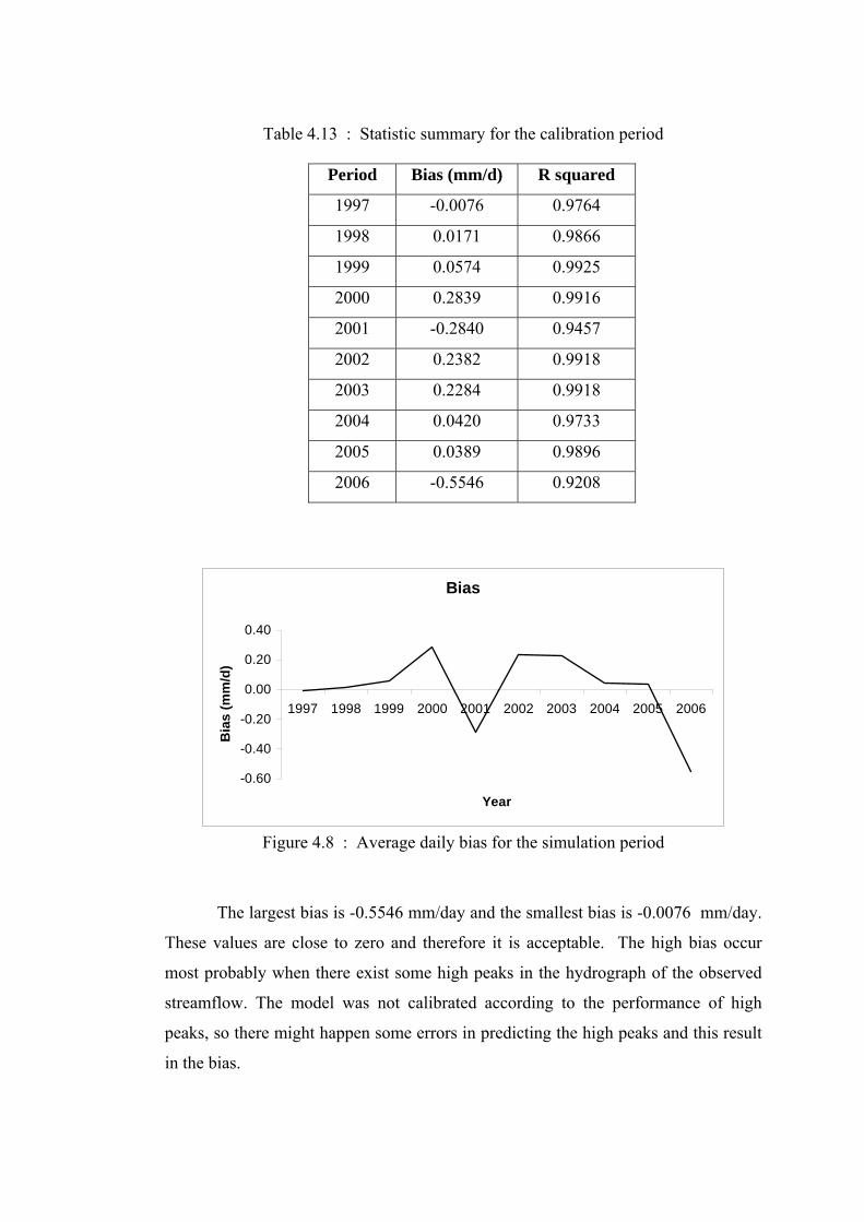
Table 4.13 : Statistic summary for the calibration period

Period Bias (mm/d) R squared

1997 -0.0076 0.9764

1998 0.0171 0.9866

1999 0.0574 0.9925

2000 0.2839 0.9916

2001 -0.2840 0.9457

2002 0.2382 0.9918

2003 0.2284 0.9918

2004 0.0420 0.9733

2005 0.0389 0.9896

2006 -0.5546 0.9208

Bias

-0.60

-0.40

-0.20

0.00

0.20

0.40

1997 1998 1999 2000 2001 2002 2003 2004 2005 2006

Year

Bia

s (m

m/d

)

Figure 4.8 : Average daily bias for the simulation period

The largest bias is -0.5546 mm/day and the smallest bias is -0.0076 mm/day.

These values are close to zero and therefore it is acceptable. The high bias occur

most probably when there exist some high peaks in the hydrograph of the observed

streamflow. The model was not calibrated according to the performance of high

peaks, so there might happen some errors in predicting the high peaks and this result

in the bias.

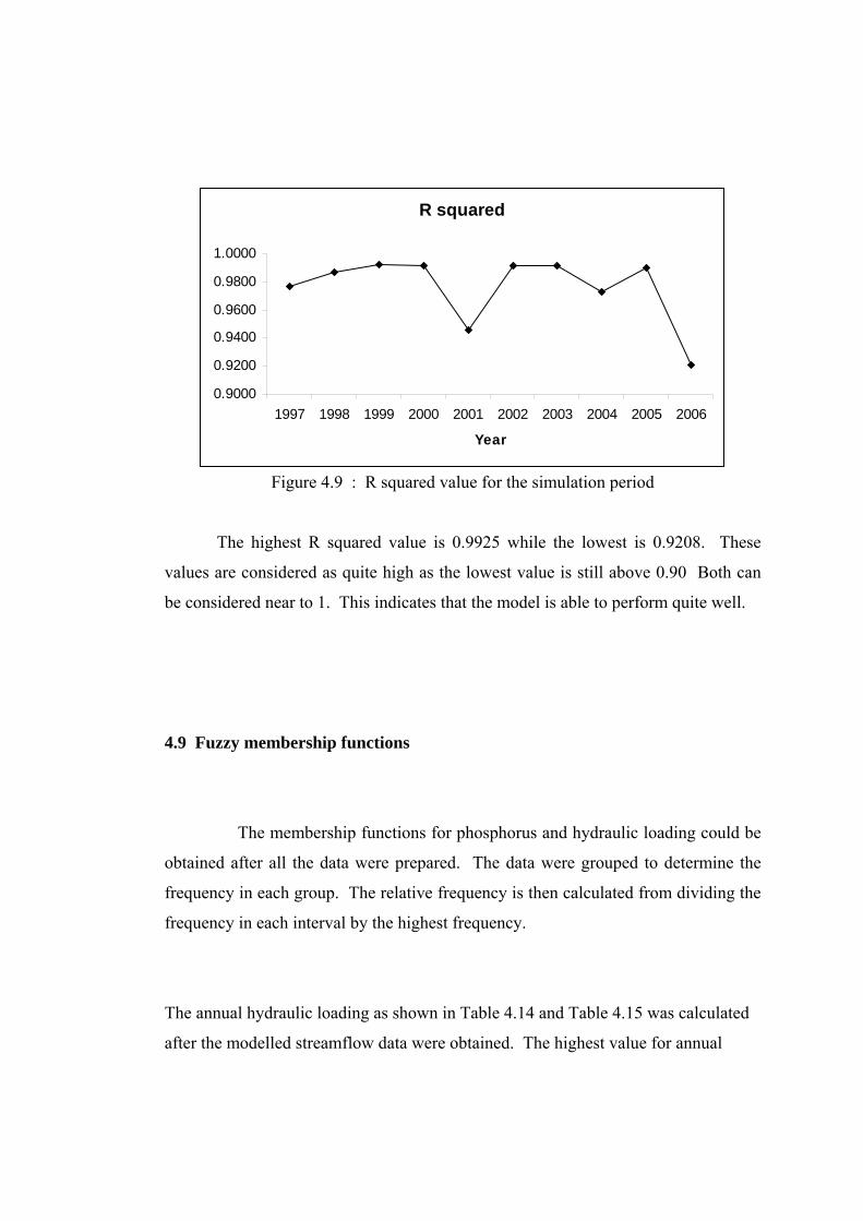
R squared

0.9000

0.9200

0.9400

0.9600

0.9800

1.0000

1997 1998 1999 2000 2001 2002 2003 2004 2005 2006

Year

Figure 4.9 : R squared value for the simulation period

The highest R squared value is 0.9925 while the lowest is 0.9208. These

values are considered as quite high as the lowest value is still above 0.90 Both can

be considered near to 1. This indicates that the model is able to perform quite well.

4.9 Fuzzy membership functions

The membership functions for phosphorus and hydraulic loading could be

obtained after all the data were prepared. The data were grouped to determine the

frequency in each group. The relative frequency is then calculated from dividing the

frequency in each interval by the highest frequency.

The annual hydraulic loading as shown in Table 4.14 and Table 4.15 was calculated

after the modelled streamflow data were obtained. The highest value for annual

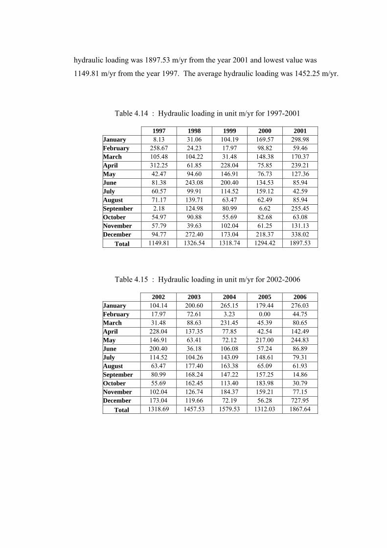
hydraulic loading was 1897.53 m/yr from the year 2001 and lowest value was

1149.81 m/yr from the year 1997. The average hydraulic loading was 1452.25 m/yr.

Table 4.14 : Hydraulic loading in unit m/yr for 1997-2001

1997 1998 1999 2000 2001 January 8.13 31.06 104.19 169.57 298.98 February 258.67 24.23 17.97 98.82 59.46 March 105.48 104.22 31.48 148.38 170.37 April 312.25 61.85 228.04 75.85 239.21 May 42.47 94.60 146.91 76.73 127.36 June 81.38 243.08 200.40 134.53 85.94 July 60.57 99.91 114.52 159.12 42.59 August 71.17 139.71 63.47 62.49 85.94 September 2.18 124.98 80.99 6.62 255.45 October 54.97 90.88 55.69 82.68 63.08 November 57.79 39.63 102.04 61.25 131.13 December 94.77 272.40 173.04 218.37 338.02

Total 1149.81 1326.54 1318.74 1294.42 1897.53

Table 4.15 : Hydraulic loading in unit m/yr for 2002-2006

2002 2003 2004 2005 2006 January 104.14 200.60 265.15 179.44 276.03 February 17.97 72.61 3.23 0.00 44.75 March 31.48 88.63 231.45 45.39 80.65 April 228.04 137.35 77.85 42.54 142.49 May 146.91 63.41 72.12 217.00 244.83 June 200.40 36.18 106.08 57.24 86.89 July 114.52 104.26 143.09 148.61 79.31 August 63.47 177.40 163.38 65.09 61.93 September 80.99 168.24 147.22 157.25 14.86 October 55.69 162.45 113.40 183.98 30.79 November 102.04 126.74 184.37 159.21 77.15 December 173.04 119.66 72.19 56.28 727.95

Total 1318.69 1457.53 1579.53 1312.03 1867.64

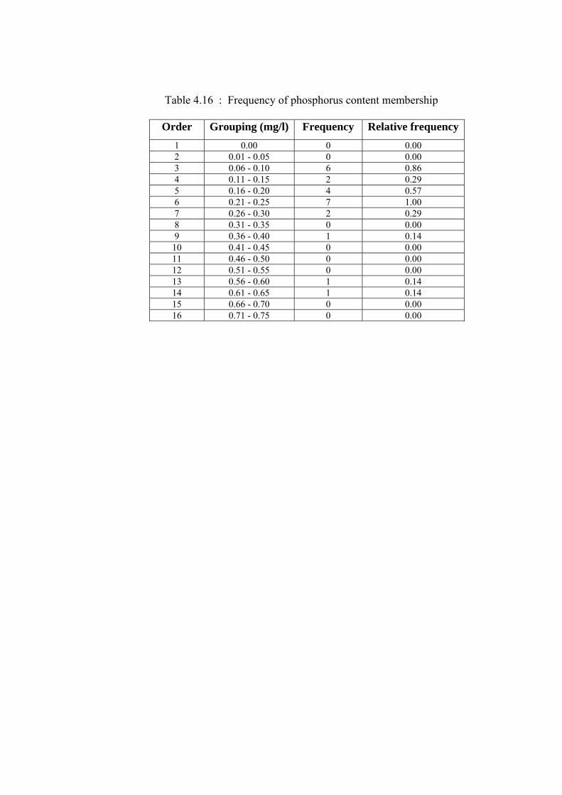
Table 4.16 : Frequency of phosphorus content membership

Order Grouping (mg/l) Frequency Relative frequency

1 0.00 0 0.00 2 0.01 - 0.05 0 0.00 3 0.06 - 0.10 6 0.86 4 0.11 - 0.15 2 0.29 5 0.16 - 0.20 4 0.57 6 0.21 - 0.25 7 1.00 7 0.26 - 0.30 2 0.29 8 0.31 - 0.35 0 0.00 9 0.36 - 0.40 1 0.14

10 0.41 - 0.45 0 0.00 11 0.46 - 0.50 0 0.00 12 0.51 - 0.55 0 0.00 13 0.56 - 0.60 1 0.14 14 0.61 - 0.65 1 0.14 15 0.66 - 0.70 0 0.00 16 0.71 - 0.75 0 0.00

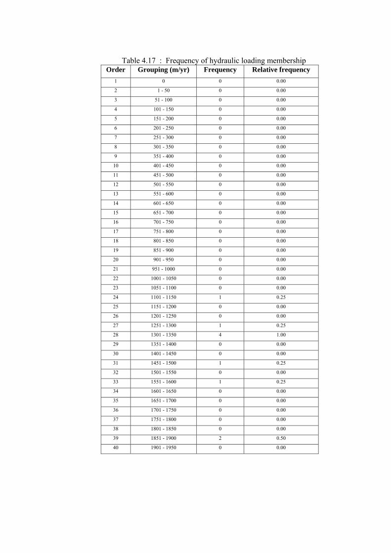
Table 4.17 : Frequency of hydraulic loading membership Order Grouping (m/yr) Frequency Relative frequency

1 0 0 0.00

2 1 - 50 0 0.00

3 51 - 100 0 0.00

4 101 - 150 0 0.00

5 151 - 200 0 0.00

6 201 - 250 0 0.00

7 251 - 300 0 0.00

8 301 - 350 0 0.00

9 351 - 400 0 0.00

10 401 - 450 0 0.00

11 451 - 500 0 0.00

12 501 - 550 0 0.00

13 551 - 600 0 0.00

14 601 - 650 0 0.00

15 651 - 700 0 0.00

16 701 - 750 0 0.00

17 751 - 800 0 0.00

18 801 - 850 0 0.00

19 851 - 900 0 0.00

20 901 - 950 0 0.00

21 951 - 1000 0 0.00

22 1001 - 1050 0 0.00

23 1051 - 1100 0 0.00

24 1101 - 1150 1 0.25

25 1151 - 1200 0 0.00

26 1201 - 1250 0 0.00

27 1251 - 1300 1 0.25

28 1301 - 1350 4 1.00

29 1351 - 1400 0 0.00

30 1401 - 1450 0 0.00

31 1451 - 1500 1 0.25

32 1501 - 1550 0 0.00

33 1551 - 1600 1 0.25

34 1601 - 1650 0 0.00

35 1651 - 1700 0 0.00

36 1701 - 1750 0 0.00

37 1751 - 1800 0 0.00

38 1801 - 1850 0 0.00

39 1851 - 1900 2 0.50

40 1901 - 1950 0 0.00

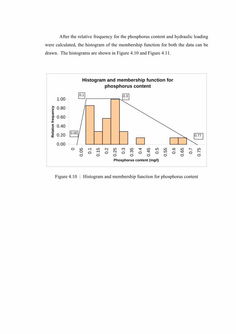
After the relative frequency for the phosphorus content and hydraulic loading

were calculated, the histogram of the membership function for both the data can be

drawn. The histograms are shown in Figure 4.10 and Figure 4.11.

Histogram and membership function for phosphorus content

0.00

0.20

0.40

0.60

0.80

1.00

0

0.05 0.

1

0.15 0.

2

0.25 0.

3

0.35 0.

4

0.45 0.

5

0.55 0.

6

0.65 0.

7

0.75

Phosphorus content (mg/l)

Rel

ativ

e fr

eque

ncy

0.1

0.77

0.3

0.05

Figure 4.10 : Histogram and membership function for phosphorus content

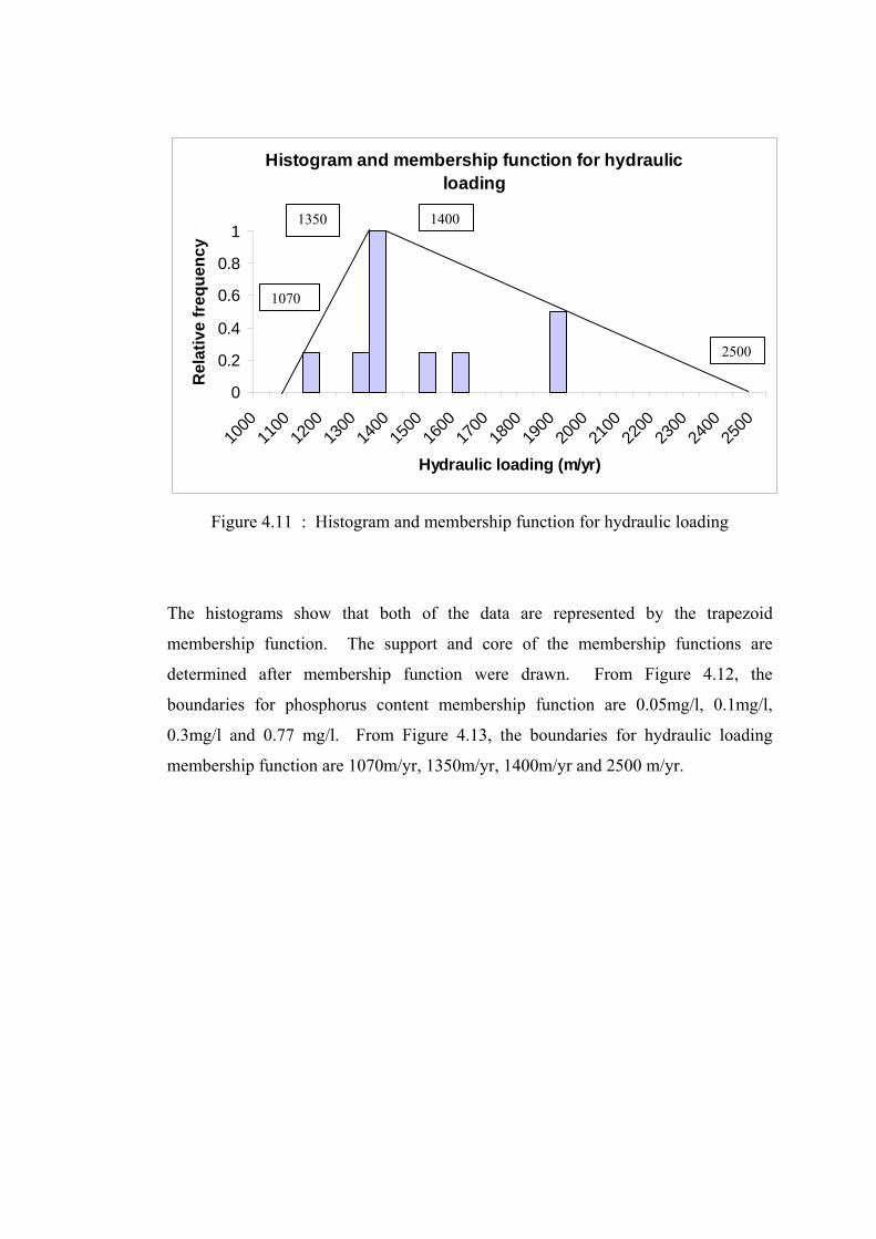
Histogram and membership function for hydraulic loading

0

0.2

0.4

0.6

0.8

1

1000

1100

1200

1300

1400

1500

1600

1700

1800

1900

2000

2100

2200

2300

2400

2500

Hydraulic loading (m/yr)

Rel

ativ

e fr

eque

ncy

14001350

1070

2500

Figure 4.11 : Histogram and membership function for hydraulic loading

The histograms show that both of the data are represented by the trapezoid

membership function. The support and core of the membership functions are

determined after membership function were drawn. From Figure 4.12, the

boundaries for phosphorus content membership function are 0.05mg/l, 0.1mg/l,

0.3mg/l and 0.77 mg/l. From Figure 4.13, the boundaries for hydraulic loading

membership function are 1070m/yr, 1350m/yr, 1400m/yr and 2500 m/yr.

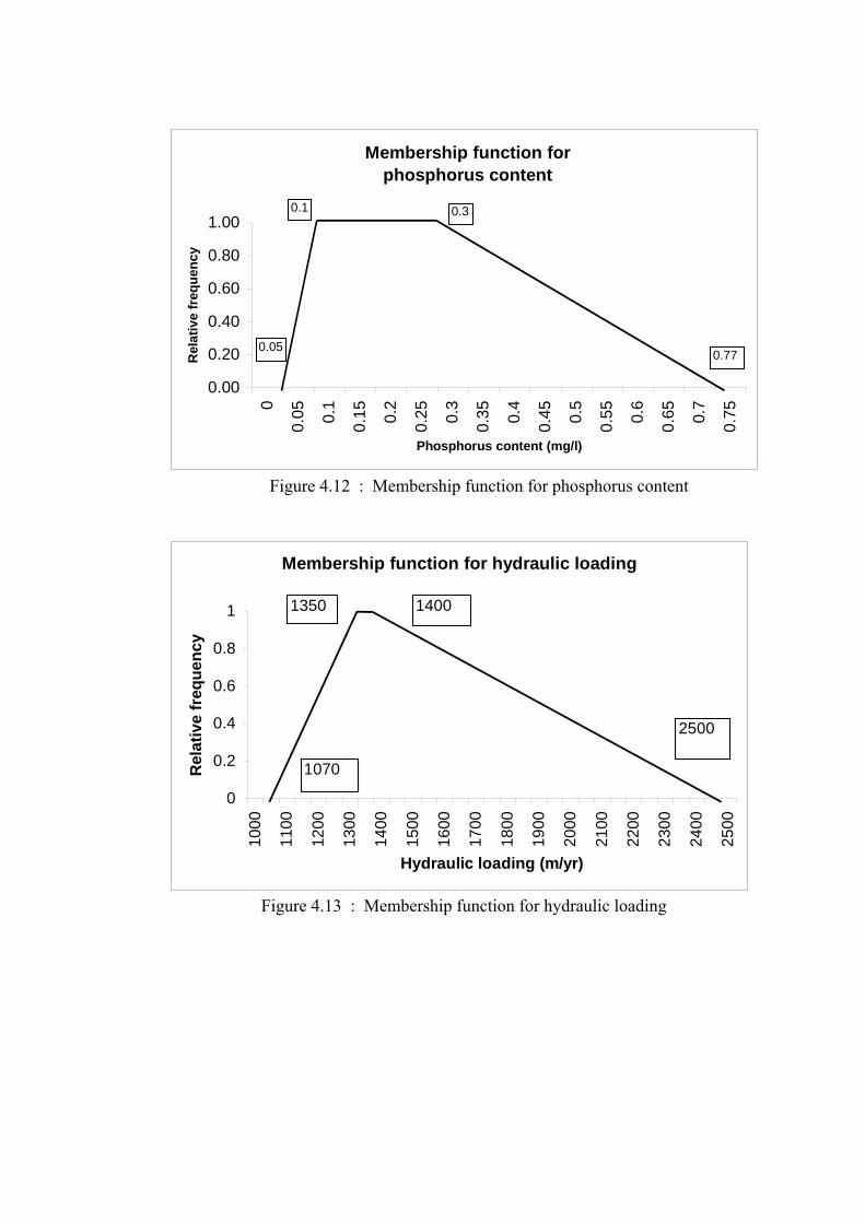
Membership function for phosphorus content

0.00

0.20

0.40

0.60

0.80

1.00

0

0.05 0.

1

0.15 0.

2

0.25 0.

3

0.35 0.

4

0.45 0.

5

0.55 0.

6

0.65 0.

7

0.75

Phosphorus content (mg/l)

Rel

ativ

e fr

eque

ncy

0.1

0.77

0.3

0.05

Figure 4.12 : Membership function for phosphorus content

Membership function for hydraulic loading

0

0.2

0.4

0.6

0.8

1

1000

1100

1200

1300

1400

1500

1600

1700

1800

1900

2000

2100

2200

2300

2400

2500

Hydraulic loading (m/yr)

Rel

ativ

e fr

eque

ncy

14001350

2500

1070

Figure 4.13 : Membership function for hydraulic loading

From the Vollenweider model as in Equation 3.1, P is represented by the

membership function for phosphorus content and qs is represented by the

membership function for hydraulic loading. The Tw value used is 0.86 yr (Supiah,

1997). The membership function for the phosphorus loading are determined by

using arithmetic operation as in Equation 3.18. The operation is done to find the core

and support of the phosphorus loading membership function. [a,b] represent the

interval number in membership function for phosphorus content, while [c,d]

represent the interval number membership function for hydraulic loading. The

membership function for phosphorus loading is shown in Figure 4.14.

At the core,

[a,b] • [c,d] = [0.1, 0.3] • [1350, 1400]

= [min (135, 140, 405, 420), max (135, 140, 405, 420)]

= [135, 420]

At the support,

[a,b] • [c,d] = [0.05, 0.77] • [1070, 2500]

= [min (53.5, 125, 823.9, 1925), max (53.5, 125, 823.9, 1295)]

= [53.5, 1925]

Example of calculation:

At the support,

Lp = P . qs . (1 + √ Tw )

= 53.5 . (1 + √ Tw )

= 53.5 . (1 + √ 0.86 )

= 100 mg/m2/yr

= 0.1 g/m2/yr

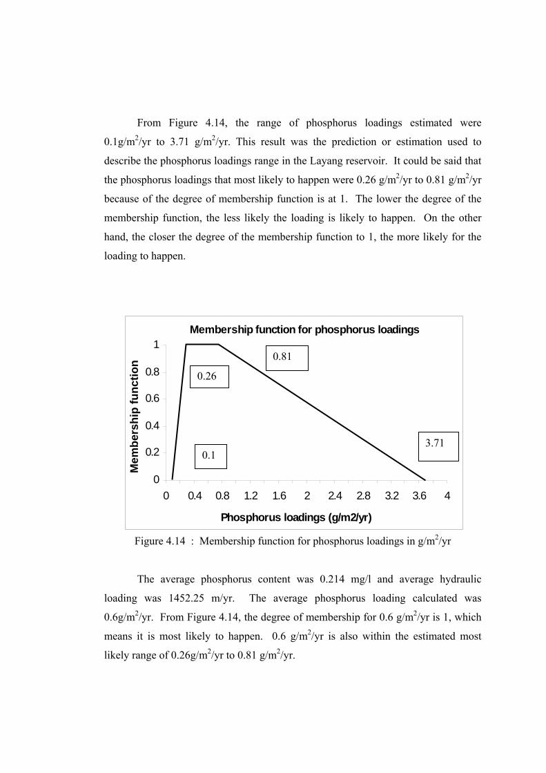
From Figure 4.14, the range of phosphorus loadings estimated were

0.1g/m2/yr to 3.71 g/m2/yr. This result was the prediction or estimation used to

describe the phosphorus loadings range in the Layang reservoir. It could be said that

the phosphorus loadings that most likely to happen were 0.26 g/m2/yr to 0.81 g/m2/yr

because of the degree of membership function is at 1. The lower the degree of the

membership function, the less likely the loading is likely to happen. On the other

hand, the closer the degree of the membership function to 1, the more likely for the

loading to happen.

Membership function for phosphorus loadings

0

0.2

0.4

0.6

0.8

1

0 0.4 0.8 1.2 1.6 2 2.4 2.8 3.2 3.6 4

Phosphorus loadings (g/m2/yr)

Mem

bers

hip

func

tion

0.81

0.26

3.71 0.1

Figure 4.14 : Membership function for phosphorus loadings in g/m2/yr The average phosphorus content was 0.214 mg/l and average hydraulic

loading was 1452.25 m/yr. The average phosphorus loading calculated was

0.6g/m2/yr. From Figure 4.14, the degree of membership for 0.6 g/m2/yr is 1, which

means it is most likely to happen. 0.6 g/m2/yr is also within the estimated most

likely range of 0.26g/m2/yr to 0.81 g/m2/yr.

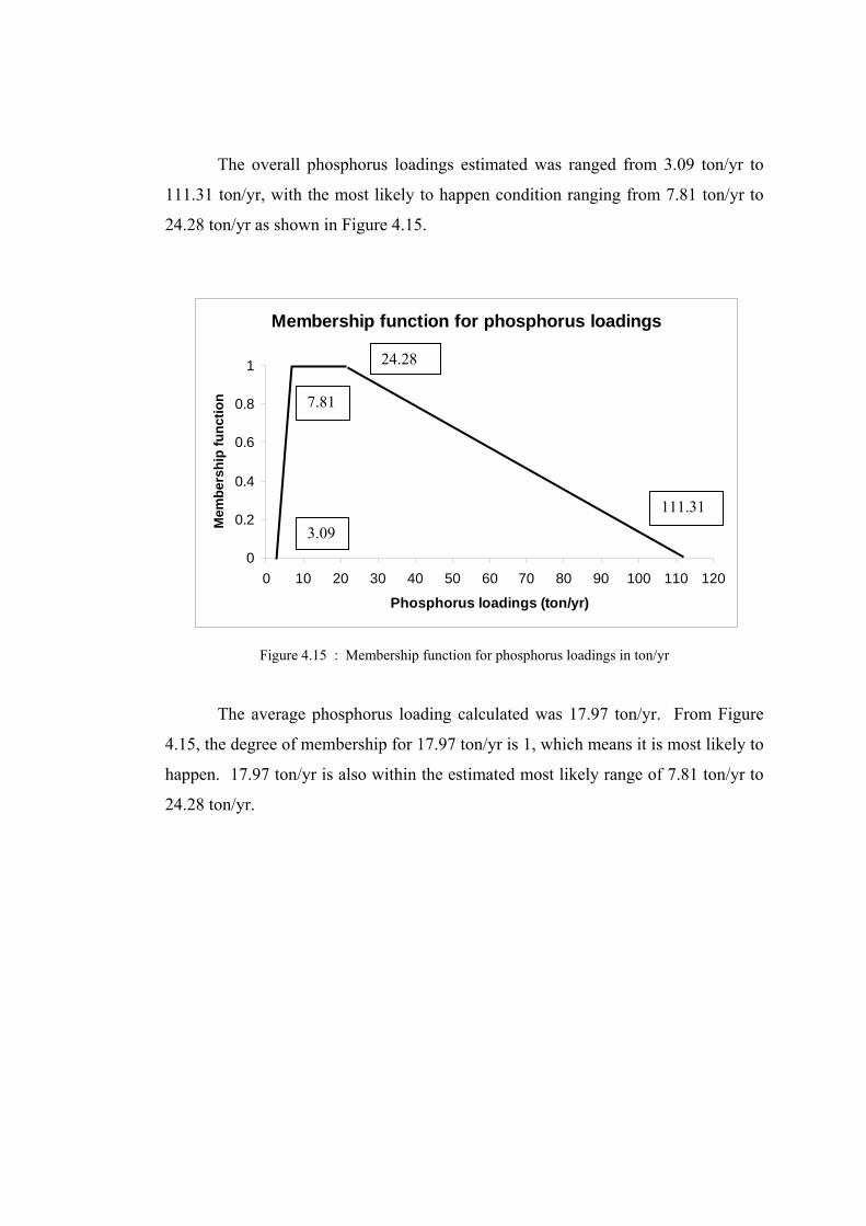
The overall phosphorus loadings estimated was ranged from 3.09 ton/yr to

111.31 ton/yr, with the most likely to happen condition ranging from 7.81 ton/yr to

24.28 ton/yr as shown in Figure 4.15.

Membership function for phosphorus loadings

0

0.2

0.4

0.6

0.8

1

0 10 20 30 40 50 60 70 80 90 100 110 120

Phosphorus loadings (ton/yr)

Mem

bers

hip

func

tion

24.28

7.81

111.31 3.09

Figure 4.15 : Membership function for phosphorus loadings in ton/yr The average phosphorus loading calculated was 17.97 ton/yr. From Figure

4.15, the degree of membership for 17.97 ton/yr is 1, which means it is most likely to

happen. 17.97 ton/yr is also within the estimated most likely range of 7.81 ton/yr to

24.28 ton/yr.

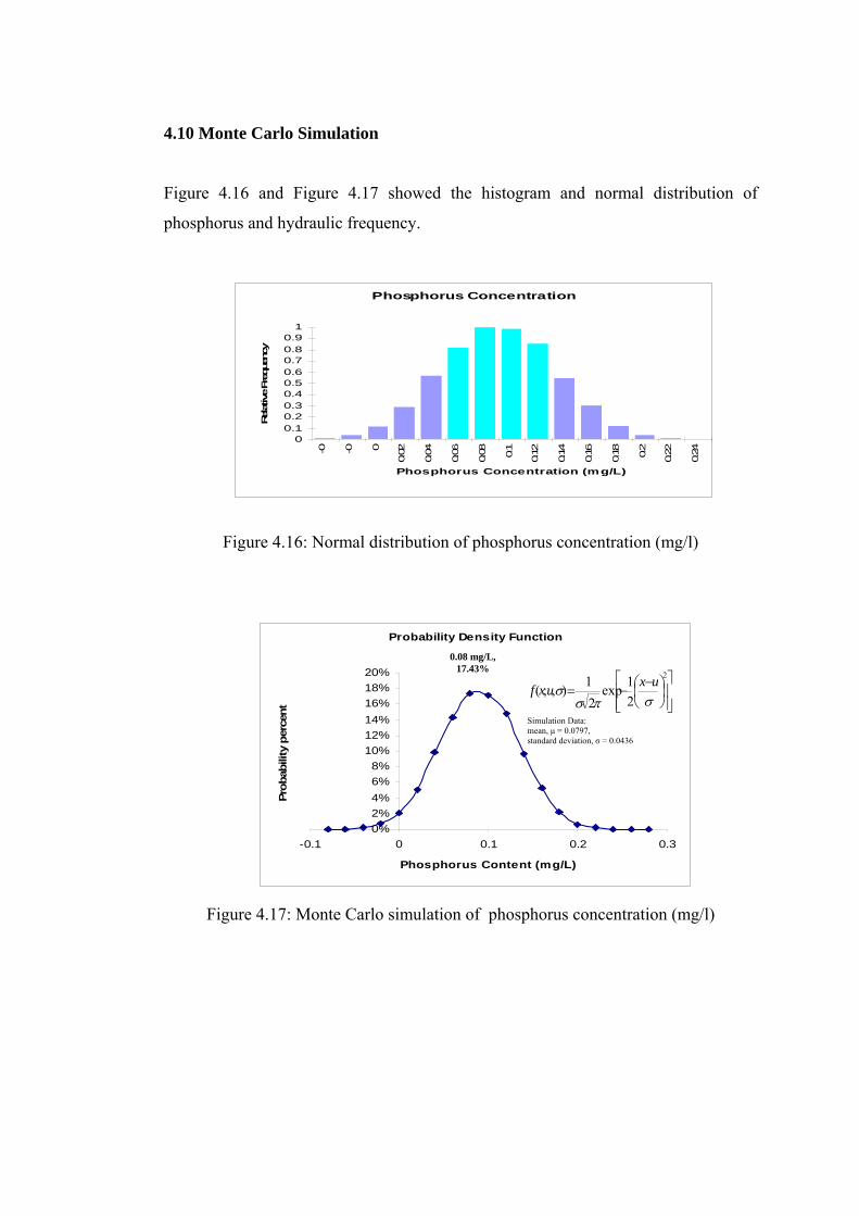
4.10 Monte Carlo Simulation

Figure 4.16 and Figure 4.17 showed the histogram and normal distribution of

phosphorus and hydraulic frequency.

Phosphorus Concentration

00.10.20.30.40.50.60.70.80.9

1-0 -0 0

0.02

0.04

0.06

0.08 0.1

0.12

0.14

0.16

0.18 0.2

0.22

0.24

Phosphorus Concentration (mg/L)

Relat

ive Fr

eque

ncy

Figure 4.16: Normal distribution of phosphorus concentration (mg/l)

Probability Density Function

0%2%4%6%8%

10%12%14%16%18%20%

-0.1 0 0.1 0.2 0.3

Phosphorus Content (mg/L)

Prob

abili

ty p

erce

nt ⎥⎥⎦

⎤

⎢⎢⎣

⎡⎟⎠⎞

⎜⎝⎛ −

−=2

21exp

21),;(

σπσσ uxuxf

0.08 mg/L, 17.43%

Simulation Data: mean, µ = 0.0797, standard deviation, σ = 0.0436

Figure 4.17: Monte Carlo simulation of phosphorus concentration (mg/l)

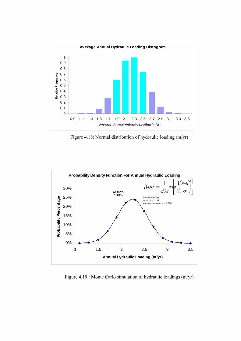
Average Annual Hydraulic Loading Histogram

00.10.20.30.40.50.60.70.80.9

1

0.9 1.1 1.3 1.5 1.7 1.9 2.1 2.3 2.5 2.7 2.9 3.1 3.3 3.5Average Annual Hydraulic Loading (m/yr)

Rel

ativ

e Fr

eque

ncy

Figure 4.18: Normal distribution of hydraulic loading (m/yr)

Probability Density Function For Annual Hydraulic Loading

0%

5%

10%

15%

20%

25%

30%

1 1.5 2 2.5 3 3.5

Annual Hydraulic Loading (m/yr)

Prob

abili

ty P

erce

ntag

e

⎥⎥⎦

⎤

⎢⎢⎣

⎡⎟⎠⎞

⎜⎝⎛ −−=

2

21exp

21),;(

σπσσ uxuxf

2.3 m/yr, 23.80%

Simulation Data: mean, µ = 2.134, standard deviation, σ = 0.320

Figure 4.19 : Monte Carlo simulation of hydraulic loadings (m/yr)

Figure 4.16, showed the most likely range of phosphorus content obtained

was 0.06 mg/l to 0.12 mg/l based on 4 highest histogram. The average phosphorus

content was 0.0801 mg/l from Monte Carlo probability density function with

probability percentage as many as 17.43% through normal distribution using

phosphorus (mg/l) average simulation data of 0.0797 mg/l and standard deviation

0.0436.

Figure 4.18, the most likely range of annual hydraulic loading was 1.9 m/yr

to 2.5 m/yr based on 4 highest histogram. The average annual hydraulic loading was

2.134 m/yr from Monte Carlo probability density function with probability

percentage as many as 23.80% through normal distribution using hydraulic loading

(m/yr) data simulation average of 2.134 m/yr and standard deviation 0.320.

To get the annual phosphorus loading, the two range and mean of phosphorus

and hydraulic loading are combined through simple multiplication. The average

phosphorus loadings obtained was 0.330 g/m2/yr (10.065 ton/yr), within the

estimated range of 0.220 g/m2/yr to 0.578 g/m2/yr (6.710 ton/yr to 17.629 ton/yr).

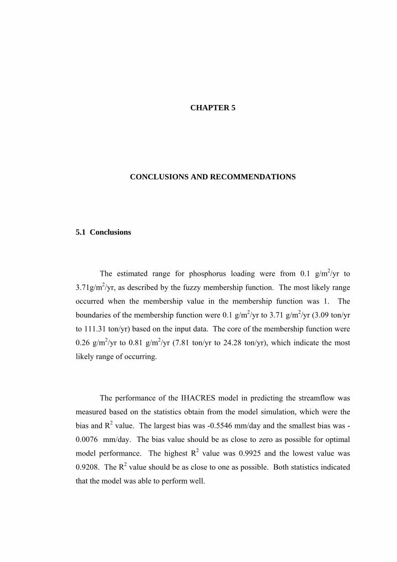
CHAPTER 5

CONCLUSIONS AND RECOMMENDATIONS

5.1 Conclusions

The estimated range for phosphorus loading were from 0.1 g/m2/yr to

3.71g/m2/yr, as described by the fuzzy membership function. The most likely range

occurred when the membership value in the membership function was 1. The

boundaries of the membership function were 0.1 g/m2/yr to 3.71 g/m2/yr (3.09 ton/yr

to 111.31 ton/yr) based on the input data. The core of the membership function were

0.26 g/m2/yr to 0.81 g/m2/yr (7.81 ton/yr to 24.28 ton/yr), which indicate the most

likely range of occurring.

The performance of the IHACRES model in predicting the streamflow was

measured based on the statistics obtain from the model simulation, which were the

bias and R2 value. The largest bias was -0.5546 mm/day and the smallest bias was -

0.0076 mm/day. The bias value should be as close to zero as possible for optimal

model performance. The highest R2 value was 0.9925 and the lowest value was

0.9208. The R2 value should be as close to one as possible. Both statistics indicated

that the model was able to perform well.

The fuzzy membership function was developed to represent the uncertainty of

the phosphorus loadings estimation. The range of minimum and maximum values

for parameter of Vollenweider model could be obtained from the fuzzy membership

function.

The average phosphorus content was 0.0801 mg/l from Monte Carlo

probability density function with probability percentage of 17.43% through normal

distribution. The average annual hydraulic loading was 2.134 m/yr from Monte Carlo

probability density function with probability percentage of 23.80% through normal

distribution.

There were two models used in this study, which were Vollenweider model

and IHACRES model. All models were not perfect, but predictions or estimations

could be made by using the models, which could later provide a better insight

regarding to eutrophication related problems. Phosphorus loadings were expected to

increase in the future from the activities observed in the catchment area. Therefore,

proper management and mitigation were required to control the eutrophication either

at the point sources or non-point sources.

5.2 Recommendations

Some suggestions and recommendations could be made for this study to

improve the performance or the quality of the data and the results.

i) Site investigations could be done more often to increase the quantity of the data

and samples. These data would be used in fuzzy membership function to

represent the actual condition throughout the catchment area. The

representation would be more accurate when more data are collected.

ii) The stations for study could be added to increase the amount of data and set up

at various points thoughout the study area. The locations and distribution of the

stations should be arranged so that they represent the study area as a whole.

iii) Streamflow recording stations could be set up at the study area to obtain the

actual streamflow of the study area. This will increase the quality of the data

and improve the quality of the result generated.

iv) Study or research could be done in searching and obtaining computer softwares

or programs that could generate histogram and fuzzy membership functions.

This will help in saving time and increase the easiness to generate the

histograms and membership functions and also to obtain the desired results.

REFERENCES

Debarry, P. A. (2004), “Watersheds Processes, Assessment, and Management.”, New

Jersey : John Wiley & Sons, Inc.

Dong, W. and Shah, H. C. (1987), “Vertex Method for Computing Functions of

Fuzzy Variables.” Fuzzy Sets and Systems, Vol. 24 65-78.

Evans, J. P. and Jakeman, A. J. (1998), “Development of a Simple, Catchment-Scale

Rainfall-Evapotranspiration-Runoff model” Environment Modeling Software, Vol.

13, 385-393.

Faradilah Abd Rahman (2006), “Fuzzy Analysis for Vollenweider Phosphorus

Loadings Model at Layang Reservoir Systems”, Degree thesis, Universiti Teknologi

Malaysia.

Galindo, J. Urrutia, A., Piattini, M. (2006), “Fuzzy Databases Modeling, Design and

Implementation”, Hershey : Idea Group Publishing.

Hammer, M. J. and McKichan, K. A. (1981), “Hydrology and Quality of Water

Resources”, New York : John Wiley & Sons, Inc.

Herschy, Reginald W. (1995), “Streamflow Measurement”, 2nd edition, London : E

& FN Spon.

Hong X.L. and Vincent C. Y. (1995), “Fuzzy Sets and Fuzzy Decision Making”,

CRC Press.

Jakeman, A. J. and Hornberger, G. M. (1993), “How Much Complexity is Warranted

in a Rainfall-Runoff Model?” Water Resource Research, Vol. 29 2637-2649.

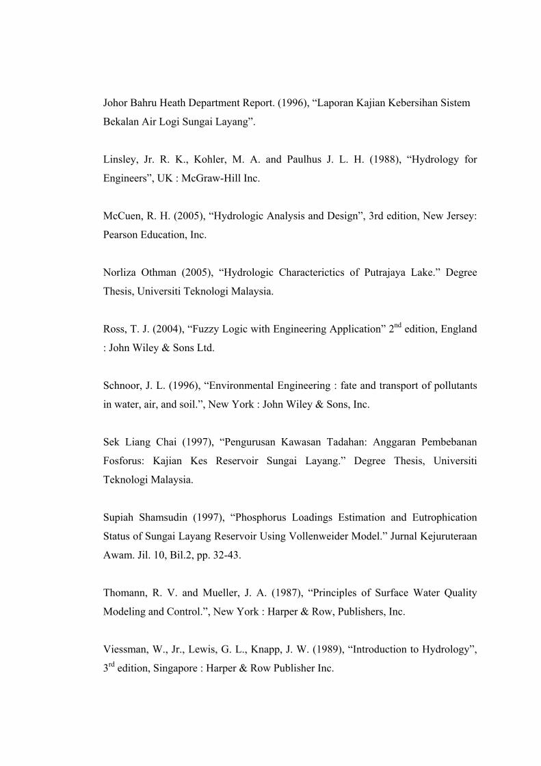
Johor Bahru Heath Department Report. (1996), “Laporan Kajian Kebersihan Sistem

Bekalan Air Logi Sungai Layang”.

Linsley, Jr. R. K., Kohler, M. A. and Paulhus J. L. H. (1988), “Hydrology for

Engineers”, UK : McGraw-Hill Inc.

McCuen, R. H. (2005), “Hydrologic Analysis and Design”, 3rd edition, New Jersey:

Pearson Education, Inc.

Norliza Othman (2005), “Hydrologic Characterictics of Putrajaya Lake.” Degree

Thesis, Universiti Teknologi Malaysia.

Ross, T. J. (2004), “Fuzzy Logic with Engineering Application” 2nd edition, England

: John Wiley & Sons Ltd.

Schnoor, J. L. (1996), “Environmental Engineering : fate and transport of pollutants

in water, air, and soil.”, New York : John Wiley & Sons, Inc.

Sek Liang Chai (1997), “Pengurusan Kawasan Tadahan: Anggaran Pembebanan

Fosforus: Kajian Kes Reservoir Sungai Layang.” Degree Thesis, Universiti

Teknologi Malaysia.

Supiah Shamsudin (1997), “Phosphorus Loadings Estimation and Eutrophication

Status of Sungai Layang Reservoir Using Vollenweider Model.” Jurnal Kejuruteraan

Awam. Jil. 10, Bil.2, pp. 32-43.

Thomann, R. V. and Mueller, J. A. (1987), “Principles of Surface Water Quality

Modeling and Control.”, New York : Harper & Row, Publishers, Inc.

Viessman, W., Jr., Lewis, G. L., Knapp, J. W. (1989), “Introduction to Hydrology”,

3rd edition, Singapore : Harper & Row Publisher Inc.

Wurbs, R. A. and James, W. P. (2002), “Water Resouces Engineering.”, Upper

Saddle River, NJ : Prentice Hall.

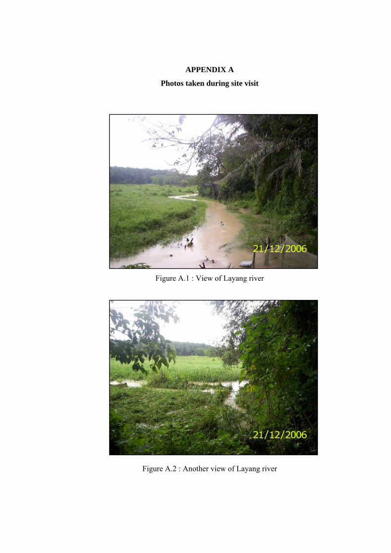
APPENDIX A

Photos taken during site visit

Figure A.1 : View of Layang river

Figure A.2 : Another view of Layang river

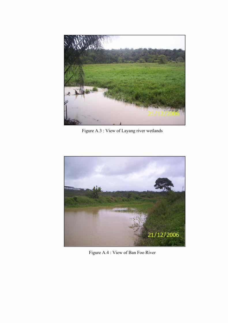
Figure A.3 : View of Layang river wetlands

Figure A.4 : View of Ban Foo River

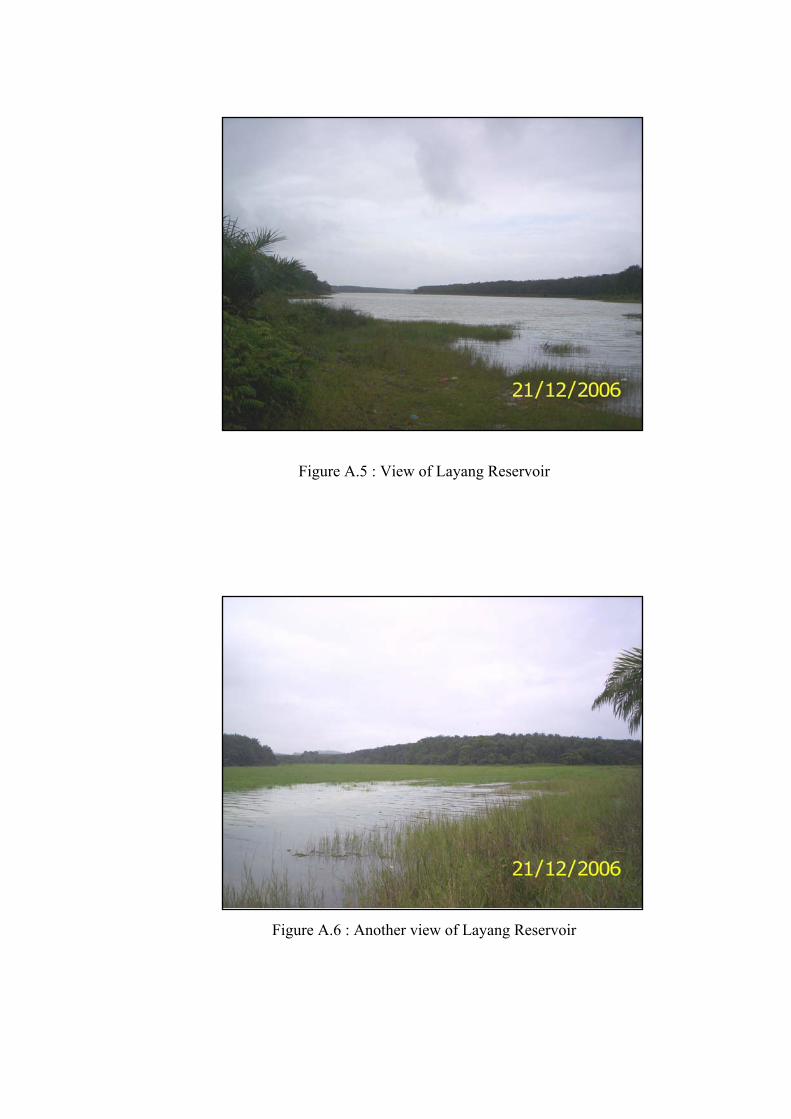
Figure A.5 : View of Layang Reservoir

Figure A.6 : Another view of Layang Reservoir

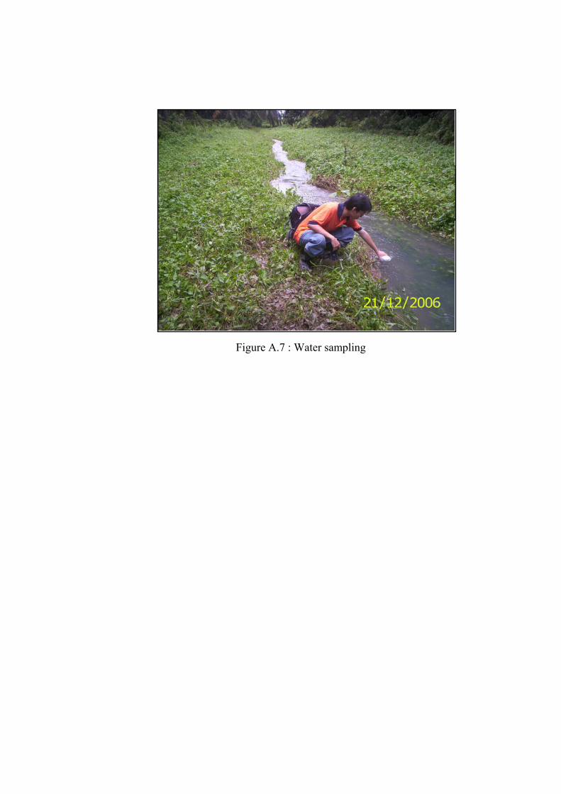
Figure A.7 : Water sampling

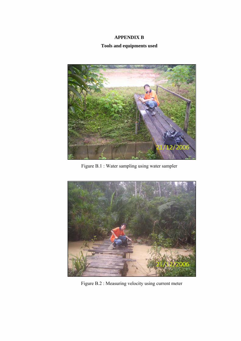
APPENDIX B

Tools and equipments used

Figure B.1 : Water sampling using water sampler

Figure B.2 : Measuring velocity using current meter

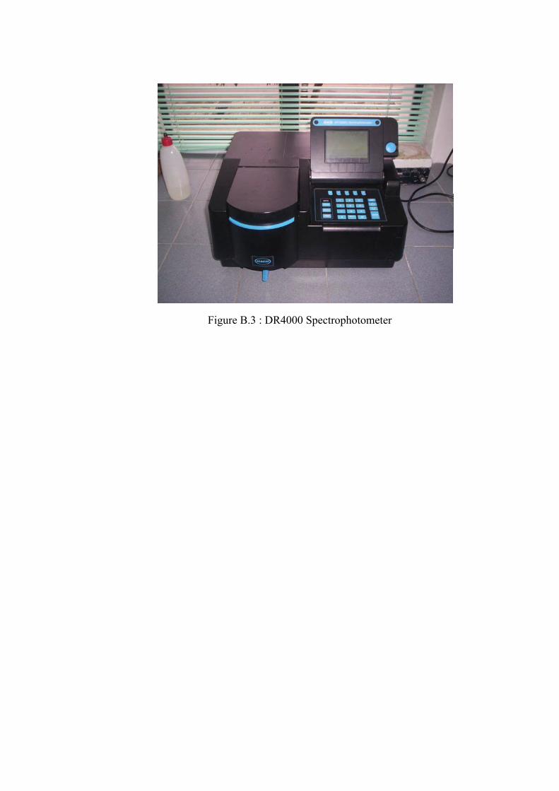
Figure B.3 : DR4000 Spectrophotometer