accepted author version posted online: 22 august 2016 ... filedalam pelbagai ekosistem. kajian ini...
TRANSCRIPT
Accepted author version posted online: 22 August 2016
Determination of Trophic Structure in Selected Freshwater Ecosystems by using Stable
Isotope Analysis
‘Amila Faqhira, Z. and Suhaila, A. H.*
School of Biological Sciences, Universiti Sains Malaysia, 11800 Penang, Malaysia
*Corresponding author: [email protected]
Abstrak: Analisis isotop stabil telah digunakan secara meluas untuk mewujudkan hubungan trofik
dalam pelbagai ekosistem. Kajian ini menggunakan tanda isotop stabil karbon dan nitrogen untuk
mengenal pasti jaringan makanan akuatik dalam ekosistem sungai dan sawah padi di Perak, utara
Semenanjung Malaysia, dan juga untuk menentukan struktur trofik jaringan makanan yang telah
dikenal pasti. Nilai min δ13C untuk semua pengeluar berjulat dari - 35.29 ± 0.21 hingga - 26.00 ±
0.050 ‰. Nilai δ15N yang terbesar terdapat dalam ikan zenarchopterid dengan 9.68 ± 0.020 ‰. Nilai
δ15N serangga akuatik berjulat antara 2.59 ± 0.107 dalam Elmidae (Coleoptera) dan 8.11 ± 0.022 ‰
dalam Nepidae (Hemiptera). Sehubungan dengan itu, dengan semua nilai δ13C dan δ15N yang telah
direkod, ia boleh disimpulkan bahawa terdapat empat tahap trofik yang wujud dalam ekosistem air
tawar yang bermula dengan pengeluar (tumbuh-tumbuhan), diikuti oleh konsumer primer (serangga
akuatik dan ikan bukan pemangsa), konsumer sekunder (pemangsa invertebrata) dan akhir sekali
konsumer tertier (pemangsa vertebrata).
Kata kunci: Tanda Isotop Stabil, Tahap Trofik, Sungai, Sawah Padi
Abstract: Stable isotope analysis has been used extensively to establish trophic relationships in
many ecosystems. Present study utilised stable isotope signatures of carbon and nitrogen to identify
trophic structure of aquatic food web in river and rice field ecosystems in Perak, northern peninsular
Malaysia. The mean δ13C values of all producers ranged from - 35.29 ± 0.21 to - 26.00 ± 0.050 ‰.
The greatest δ15N values noted was in zenarchopterid fish with 9.68 ± 0.020 ‰. The δ15N values of
aquatic insects ranged between 2.59 ± 0.107 in Elmidae (Coleoptera) and 8.11 ± 0.022 ‰ in Nepidae
(Hemiptera). Correspondingly, with all the δ13C and δ15N values recorded, it can be deduced that
there are four trophic levels existed in the freshwater ecosystems which started with the producer
(plants), followed by primary consumer (aquatic insects and non-predatory fish), secondary consumer
(invertebrate predators) and lastly tertiary consumer (vertebrate predators).
Keywords: Stable Isotope Signature, Trophic Level, River, Rice Field
INTRODUCTION
Freshwater ecosystems include rivers, streams, lakes, freshwater swamps, peat swamps, rice fields
and pools. As rivers flowing to low reaches, their water quality, substrates and food sources for
aquatic organisms altered as well. Food web studies have been used to understand linkage in energy
flow between aquatic ecosystems and terrestrial ecosystems and integrate organic matter processing
(Hershey et al., 2010). Different food sources are consumed by different faunas due to their
morphology, digestibility and the hydrology.
The stable isotope approach has become broadly used in ecology study, providing the
possibility of obtaining objective and repeatable measures of trophic position, food chain and length
omnivory (Cabana & Rasmussen, 1994). The isotopic approach is based on isotopic concentration in
the consumers’ tissues that resemble the isotopic composition in their diet (De Niro & Epstein, 1978,
1981; Peterson & Fry, 1987), which create of the relative contributions of isotopically different sources
to the consumers’ diet (Fry, 2006). Stable isotope of carbon (δ13C) is used to identify the ultimate
source of carbon, or the primary energy source for a group of organisms or for an ecosystem (Fry &
Sherr, 1984), while nitrogen (δ15N) become enriched when transferred through a food web by means
of feeding and predation (Peterson & Fry, 1987).
The study on establishment of food web structure via stable isotope analysis is neglected in
Malaysia mainly due to lack of proper facilities or instruments. Earlier findings on trophic structure was
rather general, where plants were the producers and animals were the consumers that inhabit higher
trophic level. However, this information lacks specific taxa of the organisms living in a particular
habitat, especially in rivers and paddy fields, as different species of consumer might consume
different type of food. Nevertheless, the application of stable isotope analysis was previously used to
determine nutrition of prawns in mangroves (Newell et al., 1995), food preference of the giant
mudskipper (Zulkifli et al., 2012) and food web of mudflats (Zulkifli et al., 2014). Recently, Dhiya
Shafiqah (2014) attempted to establish the food web of aquatic insects in forested tropical streams.
Therefore, this study aimed to identify the food web and to generally construct the trophic structure in
the freshwater ecosystems by using stable isotope analysis.
METHODOLOGY
Study Sites
Samples for stable isotope analysis were collected from two different water bodies of rivers and rice
fields (Fig. 1). For rivers, samples were collected from four rivers in Bukit Merah, Perak, Malaysia:
Batu Kurau River (04.54.17.400N 100.49.59.900E), Ara River (05.05.25.500N 100.51.10.700E), Jelai
River (05.00.49.800N 100.48.37.400E) and Ayer Hitam River (05.01.33.300N 100.83.49.900E). For
rice fields, samples were collected from three different rice fields in Perak, Malaysia with different
paddy growth stages: rice fields of Sg. Haji Durani (tiller phase) (03.43.40N 101.05.24E), Sg. Manik
(post-harvest phase) (04.06.027N 101.05.305E) and Kg. Felda Seberang Perak Changkat Lada
(mature phase) (04.04.805N 100.88.999E).
Sample Collection and Preparation
Ten samples in each sampling site were collected for this study. Several dominant families in each
study area were collected to represent each trophic level in their food web. Samples of plants that
represents the producer; aquatic macroinvertebrates as the primary and secondary consumer; and
fish as tertiary consumer were collected randomly in all study sites for stable isotope analysis to
compare the trophic levels in the food web. Samples preparation for the analysis was adopted from
methods described by Jardine et al. (2003) and Salas & Dudgeon (2001). All collected samples were
cleaned, oven dried at 50 – 60oC for two days and the tissues were ground into fine, homogenous
powder using a mortar and pestle. Ground samples were kept in small vials and stored in freezer until
they were analysed. Samples in powdered form were sent to Doping Control Centre (DCC) in
Universiti Sains Malaysia, analysed for stable carbon and nitrogen isotopes that was measured with
an elemental analyser (EA), connected to an isotopic-ratio mass spectrometer (IR-MS). Stable
isotope analysis followed a standard procedure by Carter and Barwick (2011). Urea isotopic working
standard (C-13, N-15) was used as the standard, while USGS40 and USGS41 (carbon and nitrogen
isotopes in L-glutamic acid) was used as isotopic reference material (RM). By following the manual
advised by Coplen (2011), USGS40 was used to plot a calibration curve of stable carbon (δ13C) and
nitrogen (δ15N). The curve was used to calculate the unknown carbon- and nitrogen- bearing
substances measured with an elemental analyzer (EA) and an isotope-ratio mass spectrometer
(IRMS) by quantifying drift with time and quantifying isotope-ratio-scale contraction when used
together with USGS41 L-glutamic acid enriched in 13C and 15N. A pair of USGS40 and USGS41 RMs
can be used at the beginning, the middle and the end of the analysis sequence to enable satisfactory
scale correction and correction of drift with time (Coplen, 2011). These reference materials and blanks
should be interspersed in between 10 – 15 samples. Each samples were replicated and measured
twice to obtain the mean for each data. Isotopic compositions of carbon and nitrogen were expressed
in δ notation (δ13C and δ15N) as part per thousand (‰) differences from international standards –
Vienna PeeDee Belemnite for carbon and atmospheric N2 for nitrogen. Stable isotope data were
expressed as the relative difference between ratios of a sample and a standard using the equation:
δ X (‰) = x 1000
where X is δ13C or δ15N and R is 13C/12C or 15N/14N of sample or standard.
Statistical Analysis
Homogeneity of variances and normality of the samples were checked in all instances. Since the data
was normally distributed, to determine where significant differences lay between the samples in the
rivers and paddy fields and between trophic level, one-way ANOVA for each sample were tested with
Tukey post hoc tests, for both δ 13C and δ 15N.
RESULTS
Stable isotope analysis was conducted on biological samples of plants, aquatic insects and fish
available from the study areas. For each sample, the mean δ15N and δ13C values obtained displayed
various degree of trophic position occurred in the rivers (Table 1 – 2). The mean values of δ15N
ranged between 2.59 ± 0.107 ‰ in Elmidae and 9.68 ± 0.020 ‰ in Zenarchopterid fish and for δ13C
values ranged from – 33.08 ± 0.210 ‰ in Heptageniidae to – 15.03 ± 0.022 ‰ in Tipulidae.
The δ15N values of vertebrate predators, i.e., fish recorded the greatest δ15N values among all
consumers. As the values of δ15N increased with the increasing trophic levels, δ15N values of fish
predators ranged between 7.63 ± 0.073 and 9.68 ± 0.020 ‰, which made them occupied the highest
trophic level cum top predator and tertiary consumers in the aquatic food web (Fig. 2). While the
invertebrate predators, mostly the plecopterans, odonates and hemipterans scored δ15N values
between 4.10 ± 0.010 and 8.11 ± 0.022 ‰, which made them lined below trophic level of fish, making
them the secondary consumers in the food web. Following below them was the primary consumers,
which were generally the herbivorous aquatic insects. They ranged from 2.59 ± 0.107 to 6.42 ±
0.214 ‰.
The δ13C signatures connote the significance of allochthonous and autochthonous sources of
carbon. Assorted allochthonous leaf litters and autochthonous algae and aquatic macrophytes were
expected to be the main basal food sources for the aquatic insects in the rivers. The average δ13C
values for the leaf litters ranged from - 31.11 ± 0.052 to - 29.62 ± 0.012 ‰, while the autochthonous
sources ranged between - 26.00 ± 0.050 and - 27.97 ± 0.125. So apparently, the amount of carbon in
autochthonous food sources were greater than the allochthonous sources.
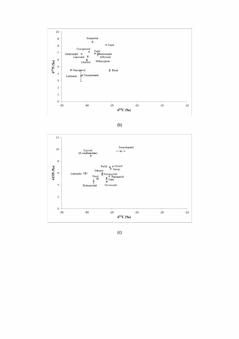
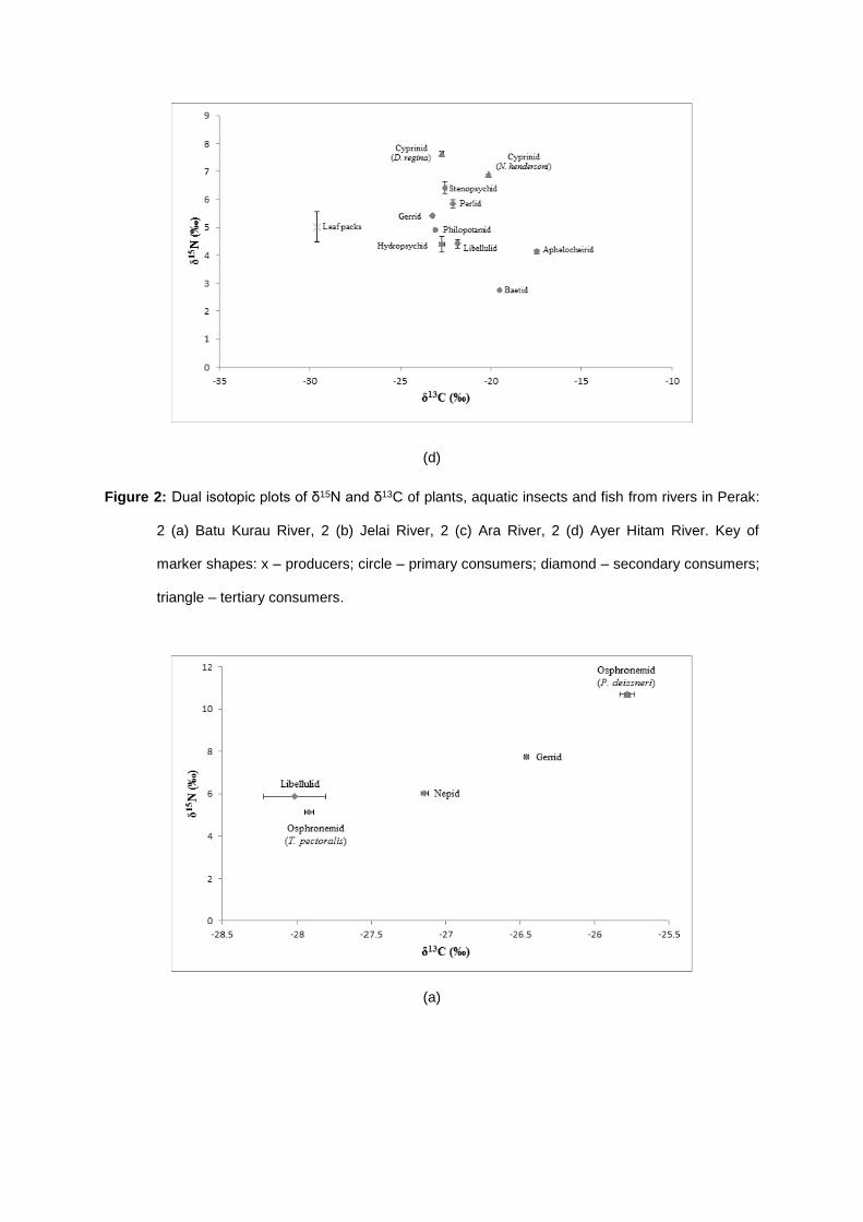
Dual isotopic plot of carbon and nitrogen in Fig. 2 illustrates the energy flow and trophic
structure of all organic samples available in the rivers. In this dual plot, the organic plants were
expected to be the main local primary producers. By referring to Fig. 2, the nitrogen and carbon
signatures of all aquatic insects were clumped closely together, ranging from 2.59 ± 0.107 to 8.11 ±
0.022 ‰ for δ15N signatures and from - 15.03 ± 0.022 to - 33.08 ± 0.210 for δ13C signatures. Hence,
according to these carbon and nitrogen values, it suggested that there are four major trophic levels in
this river ecosystem that started with the primary producers, followed by the herbivorous aquatic
insects, invertebrate predators and ended with vertebrate predators. In other terms, plants aquatic
insects aquatic insect predators fish predators.
Aquatic insects composition in the rice fields varied considerably from that of the rivers. The
aquatic insects that inhabit this type of freshwater ecosystem only consisted of collector-gatherers
and predators (Table 3 – 4). The mean values of δ15N ranged from 3.58 ± 0.16 in algae to 10.72 ±
0.05 ‰ in osphronemid fish, while the values of δ13C ranged between - 35.29 ± 0.21 in algae and -
23.59 ± 0.07 in Nepidae.
The values of δ15N of osphronemid fish, Parosphromenus deissneri recorded the greatest
δ15N values of 10.72 ± 0.05 ‰, which made them the top predators in the rice fields. The chain was
followed by the aquatic insect predators, mainly the odonates and hemipterans, with δ15N values
ranged between 2.58 ± 0.06 and 7.75 ± 0.00 ‰. Beneath this trophic level was the primary
consumers, i.e., the collectors (Chironomidae) that consume suspended particulate organic matters in
the rice fields. Algae were located at the base of the food web as the primary producer, which
contained enriched carbon (- 35.29 ± 0.21 ‰) that act as the energy source for the aquatic insects
inhabiting rice field waters.
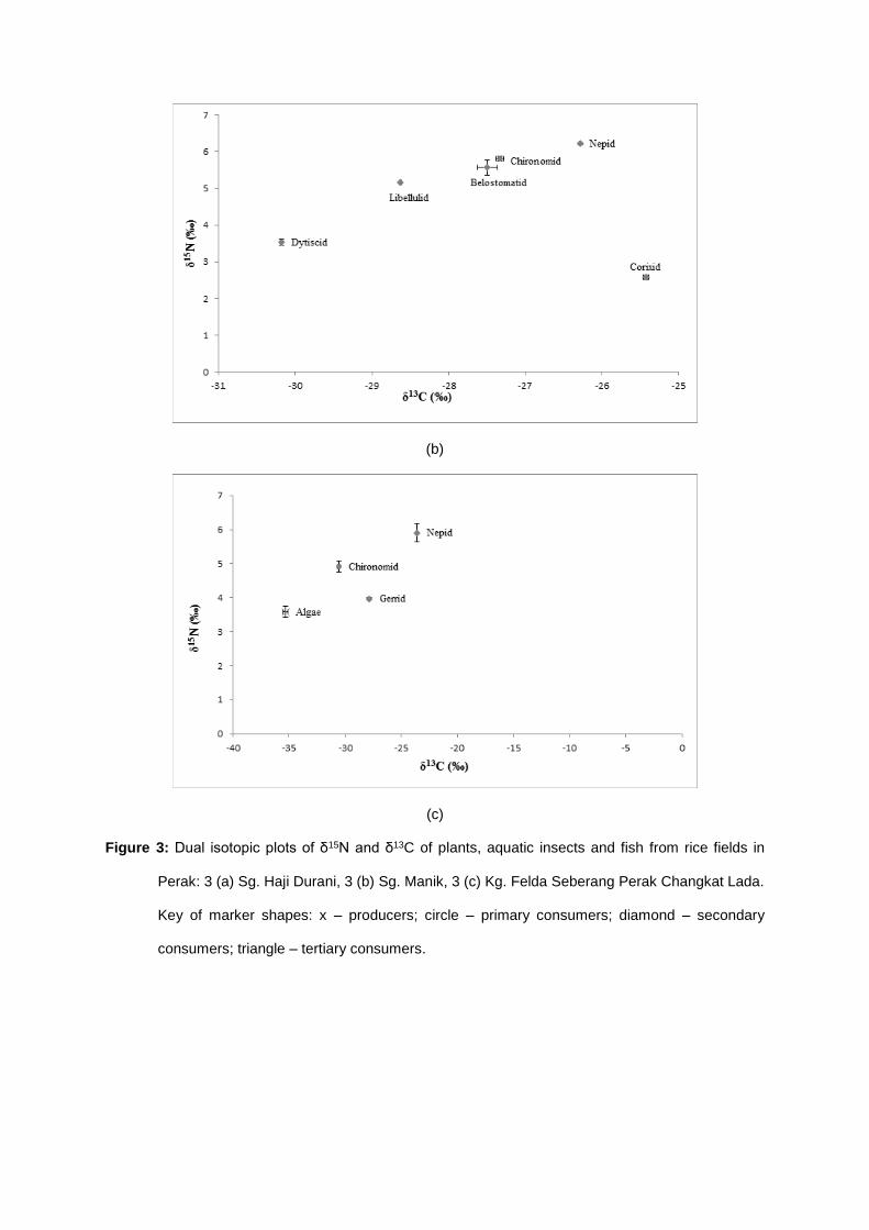
By referring to Fig. 3, algae were positioned far at the base of the trophic structure and served
as one of the main food sources. While the aquatic insects that clumped tightly on the dual isotopic
plot acted as the primary (collectors) and secondary consumers (invertebrate predators), with δ15N
ranged from 2.58 ± 0.06 to 7.75 ± 0.00 ‰ and δ13C ranged from - 30.18 ± 0.01 to - 23.59 ± 0.07 ‰.
Nevertheless, the other fish species, Trichopodus pectoralis, had lower nitrogen values, as the same
as the aquatic insects (5.12 ± 0.03 ‰) due to its herbivorous feeding mechanism. Therefore, based
on the δ15N and δ13C values plotted, it was predicted that rice fields ecosystem also consisted of four
major trophic levels, similar to river ecosystems, yet with simpler and less intricate food web,
specifically, producers aquatic insects (and non-predatory fish) aquatic insect predators fish
predators.
There was a statistically significant difference between samples in all study sites as
determined by one-way ANOVA (F (6, 62) = 2.69, P = 0.022) for δ15N and (F (6, 62) = 15.35, P = 0.000)
for δ13C. Tukey post hoc test performed on one-way ANOVA for each sample established, where the
values of δ15N and δ13C were differed between sites and trophic levels.
DISCUSSION
Analysing the stomach contents reveal the taxa of prey they consume during the right time preceding
capture of animals (Munoz-Gil et al., 2013). However, in this method the movements of nutrients and
matter through food webs and ecosystems are often difficult to observe or quantify (Polis, 1991).
Alternatively, stable isotope analysis is used to elucidate trophic relationships. Carbon and nitrogen
stable isotopes are useful to trace energy sources and food web structure in ecosystems. It also
shows the effects of anthropogenic stress on aquatic ecosystems (Bergfur et al., 2009). The stable
isotope approach is based on the similarity of isotopic concentration in the consumers’ tissues to the
stable isotopic composition of their diet (De Niro and Epstein, 1978, 1981; Peterson and Fry, 1987).
Accordingly, it establishes the relative contributions of isotopically different sources to the diet of
consumers (Fry, 2006).
The contents of both isotopes in organisms varied inconsiderably in different rivers. This
might due to the impact from the nearby land uses towards the river and different basal resources
they consumed. Changes in δ15N could specify changes in nutrient delivery to aquatic ecosystems
(Cole et al., 2004). δ15N signatures of aquatic macrophyte and algae were higher than that of the
insects suggested autochthonous origin (Salas and Dudgeon, 2001). Decreasing in stream discharge
during dry season would increase the concentrations of phosphate and nitrate in the river (Dudgeon,
1984, 1992; Dudgeon and Corlett, 1994), and hence might clarify high concentration of nitrogen in the
producers although none of the seasons was included in this study. Moreover, Thomas and Daldorph
(1994) stated that high nutrient availability is known to enhance primary production of filamentous
algae and periphyton. Next, Heptageniidae (non-predatory, herbivorous scrapers) in Ara River
contained the highest δ15N value of 5.45 ± 0.006 ‰ (4.69 ± 0.279 ‰ in Batu Kurau River; 4.50 ±
0.004 ‰ in Jelai River). During the sample collections, Ara River had numerous algae grown on the
stony substrates that act as the potential food source for the heptageniids. According to Salas and
Dudgeon (2001), high nitrogen content in the heptageniids might probably because of the abundance
of autochthonous algae grown on the stone surfaces that could provide more energy for the insects.
Such 15N-enrichment of autochthonous sources can be explained by nitrogen inputs from surrounding
orchard (Macko and Ostrom, 1994) in the human settlements. Indeed, as the nitrogen content
increased with the increasing trophic levels, the predatory Cyprinidae’s δ15N content in present study
was rather similar to the values reported for cyprinids in other study. For example, Dhiya Shafiqah
(2014) found that the cyprinids in undisturbed rivers in Royal Belum State Park scored δ15N values of
8.45 ± 0.177 ‰.
In freshwater ecosystems, the δ13C is often used to distinguish or trace the relative
importance of allochthonous and autochthonous sources of carbon (Rounick and Winterbourn, 1986).
It only shows little variation among trophic levels (Fry, 2006). Leaf litters, algae and aquatic
macrophytes were expected to be the main source of organic carbon and nutrients for the aquatic
organisms inhabiting the rivers. Among all sites sampled, Batu Kurau and Ayer Hitam rivers had more
leaf litters as compared to Jelai and Ara River (which located at higher order stream) that provide
allochthonous sources to the rivers. This can be likely linked to the shaded canopy cover in Batu
Kurau and Ayer Hitam rivers. The increased allochthonous carbon input from the surrounding riparian
vegetation in Batu Kurau and Ayer Hitam rivers would act as major source of organic carbon and
nutrients for organisms within these sites and which is lacking at higher order stream reach. Leaf
litters were also source of coarse and fine particulate organic matters for the collectors as they did not
consume the plants directly. Previous studies by England & Rosemond (2004) and Kominoski et al.
(2011) discovered that the composition of leaf litters influenced the structure and function of stream
ecosystem by altering the nutrient content and energy transfer in the food web in forest stream
ecosystem. Present study showed that leaf litters contained lower carbon signatures than the algae
and aquatic macrophytes did, as autochthonous food source had more enriched carbon than
allochthonous sources (Salas & Dudgeon, 2001). Previous studies also observed similar carbon
enrichment of autochthonous sources, as reported by Bunn et al. (1999), Dhiya Shafiqah (2014),
Lester et al. (1995) and Thorp et al. (1998).
Gregory et al. (1987) found the reduction of canopy cover had exposed stream surface to
direct sunlight and thus influenced the aquatic invertebrates to use more autotrophic energy sources.
In this study, Jelai and Ara rivers and also rice fields had open canopy covers. The increasing growth
of aquatic vegetation had interrupted the aquatic invertebrate abundance and species richness by
altering their functional role in the ecosystem, becoming the consumer of organic material and served
as preys to larger organisms (Collier, 2002; Nelson and Lieberman, 2002; Quinn et al., 1997; Suren et
al., 2003). Hence, supplementary to the allochthonous sources, as a primary producer was also
represented by other two types of autochthonous sources: aquatic macrophyte (available in Batu
Kurau and Jelai rivers) and periphytic algae (which grown abundantly in Ara River). Autochthonous
foods had higher quality (with lower C/N ratios and higher essential fatty acids contents) than leaf litter
(Lau et al., 2008, 2009) which probably accounted for their importance to consumers. In this study,
the autochthonous carbon had more 13C-enriched than allochthonous sources. Algal foods also have
a tendency to be the main energy source of stream consumers in the Neotropics (Brito et al., 2006;
Bunn et al., 1999; March and Pringle, 2003) and even in some temperate lotic ecosystems (Bunn et
al., 2003; Delong and Thorp, 2006; Torres-Ruiz et al., 2007).
Higher nutrient availability could enhance primary production of filamentous algae and
periphyton (Thomas and Daldorph, 1994) thus increasing the assimilation of dissolved inorganic
carbon (CO2). Likewise, algae were reported to be the important primary producer in autochthonous
pathway that supplied energy sources to aquatic insects (Newell et al., 1995). Consequently, 13C-
enrichment of aquatic macrophyte and algae in Batu Kurau, Jelai and Ara rivers reflect the combined
effect of light and nutrients on their growth in the environment.
In contrast to the river ecosystem, only algae were found to be the basal food sources for the
aquatic insects in rice field. Brito et al. (2006), Bunn et al. (1999) and March & Pringle (2003) stated
that algae have a tendency to be the major energy source for aquatic consumers in the Neotropics
and temperate ecosystems. The rice field offered a wide variety of conditions for the growth of algae.
Several factors including high temperature, nutrient availability, conditions of soil, humidity and the
ability of the algae to withstand desiccation (Roger and Reynaud, 1979) favour the growth of algae in
rice fields. According to Singh (1961) and Venkataraman (1972), the growth of algae contributed
significantly to spontaneous fertility of paddy soils. Fogg et al. (1973) stated that since algae are
capable of both photosynthesis and nitrogen fixation in aerobic conditions, such trophic independence
regarding carbon and nitrogen, combined with a great adaptability to variations in edaphic factors,
permits algae to be omnipresent and at the same time gives them a unique potential to contribute
productivity in a variety of agricultural and ecological situations. In this study, plants (algae in
Changkat Lada rice field) was trophically located as basal source with mean value of δ15N ~ 3.58 ±
0.16 ‰. Algae contained the most 13C-enriched food source with – 35.29 ± 0.21 ‰ thus make it an
essential primary producer in autochthonous pathway that provide energy source to the aquatic
invertebrates (Newell et al., 1995).
The use of δ15N as organisms’ trophic position tracer and organic source information
(Peterson, 1999) had shed light upon many difficulties in estimating trophic position (Vander Zanden
et al., 1997). δ15N signifies the major energy flow pathways that offer a time-integrated measure of
trophic positions, account for spatial and temporal variations in feeding at multiple levels in food web
and detect trophic interactions that are otherwise would be unnoticeable (Vander Zanden et al., 1997).
Aquatic insect family richness was greater in Batu Kurau River, later found to have the
greatest canopy cover (60 %). This suggested that increased canopy cover is related to creating more
complex habitat for a wider variety for macroinvertebrates (VanDongen et al., 2011). Increased
richness could be due to higher amounts of allochthonous input from the terrestrial landscape, which
would also account for greater representation of the shredders, collector-gatherers and collector-
filterers. The higher abundance of leaf litter in Batu Kurau and Ayer Hitam rivers created a larger
energy source for the collector-gatherers and collector-filterers, which were represented in large
number of Hydropsychidae and Stenopsychidae families. Less open areas supported the scrapers
(Vannote et al., 1980) in Batu Kurau River. The aquatic insects ranged widely in their δ13C values,
and typically were located trophically in the different level above the producers as primary and
secondary consumers, but below the tertiary consumers (vertebrate predators). The wide δ13C range
of aquatic macroinvertebrates indicated there were multiple food sources (plants or cannibalism) in
the aquatic environment (the aquatic insects carbon signatures ranged widely from – 15.03 to – 22.98
in Batu Kurau River; – 25.40 to – 33.08 in Jelai River; – 17.49 to –23.22 in Ayer Hitam River). In Ara
River, the carbon signatures of aquatic insects did not vary widely upon consumers (– 24.73 to –
28.59 δ13C). This small range of δ13C values suggested a distinct utilisation of carbon sources for
each individual.
Generally, the collector-gatherer of Elmidae (in Batu Kurau River), Neoephemeridae (in Jelai
River), Chironomidae (in Ara River) and Baetidae (in Ayer Hitam River) were located at the lowest
trophic level among all aquatic insects group. Then, followed by other aquatic insect families
comprised of different functional guilds (collector-filterer, shredder, scraper and predator). They were
clumped closely together in the dual plot because they are positioned trophically in the same level
and their large range of δ13C values implies different consumption of carbon sources for each
individual. Furthermore, unlike P. desissneri, T. pectoralis had almost the same nitrogen value as the
collector-gatherers (chironomid), which ranged between 4.91 to 5.81 ‰. This proved that T.
pectoralis did not prey on other aquatic insects; in fact, they consume mostly plant matter and algae
(Ambak et al., 2010). They are adaptable species that can survive in a wide range of biotopes;
however, they tend to thrive best in slow-moving or still waters where submerged vegetation grows
densely, for example, in rice fields, swamps and irrigation canals (Ambak et al., 2010).
In the rice fields, collector-gatherers, particularly chironomid larvae, were the common primary
consumer found in the study areas (Sg. Manik and Changkat Lada). Chironomidae are common
insects during the wet phase of the rice growing season (Al-Shami et al., 2008) and reduced in
abundance towards tiller and pre-harvest phase (Che Salmah and Abu Hassan, 2002). In this study,
the chironomid larvae present in paddy fields of Sg. Manik (post-harvest phase) and Changkat Lada
(tiller) were quite low in abundance. This functional guild generally located at the lowest trophic level
among all aquatic insects group, with δ15N ~ 5.81 ± 0.06 ‰ and 4.91 ± 0.17 ‰ in Sg. Manik and
Changkat Lada, respectively; just above the algae with mean value of δ15N ~ 3.58 ± 0.16 ‰.
Then, these primary consumers were preyed by the secondary consumers, which were the
invertebrate predators, mostly of plecopterans, odonates and hemipterans. Their nitrogen signatures
proved that they are located one trophic level above other aquatic insects, yet underneath the tertiary
consumers, or the underwater top predators: the fish. Odonates tend to consume different types of
insect to reduce prey overlapping among genera (Motta & Uieda, 2004). Moreover, Odonata are also
able to ingest various kinds of prey from different size classes (Dudgeon, 1995). On the other hand, in
this lentic ecosystem, there were only two functional feeding groups available, specifically collector-
gatherer and predator; in which differed from lotic ecosystem. During post-harvest phase in Sg. Manik,
the abundance of aquatic insect larvae was greatly reduced after the paddy plants were harvested
and the field became almost dry. During this stage, Corixidae (Hemiptera) was found in large
abundance in this rice field with 46.67 % of the total individuals collected. They inhabit standing water
and were omnivores feeding on algae, detritus and chironomid larvae (Yule and Yong, 2004). Due to
this feeding habit, they recorded the least δ15N value with 2.58 ± 0.06 ‰, which was lesser nitrogen
signature than their prey: the chironomids. Dytiscids found in Sg. Manik rice field scored mean δ15N
value of 3.54 ± 0.09 ‰ which also had lower nitrogen signature than the collector-gatherer. Even
though they were carnivores, dytiscid beetles sometimes are scavengers too depending on the
availability of the prey (Yule and Yong, 2004).
Most hemipterans and libellulids (Odonata) were the aquatic insect predators based on their
morphology and behaviour. The hemipteran families: Nepidae, Belostomatidae and Gerridae are
efficient hunters and have been known to prey on aquatic insect larvae, small fish and tadpoles
(Morse et al., 1994). They were presented at all study sites during both phases of paddy and they
prefer calm, standing water of rice fields; especially the belostomatid bugs (Yule and Yong, 2004).
Libellulids (Odonata) occurred in both paddy phases: tiller and post-harvest. They inhabit not only fast
streams and rivers but also wide range of still or sluggish waters; including pools, lakes and ponds.
Their larvae were tolerant to wide fluctuations in surrounding environment conditions for example,
temperature, oxygenation and pH (Yule and Yong, 2004). The larvae of most libellulid species are
voracious carnivores and are secretive, hiding among vegetation at the bottom (Gillott, 2005), using
their vision and/or mechanoreceptors to detect (Yule and Yong, 2004) and ambush their prey.
Naturally, the prehensile labium is shot out very rapidly to capture the target organisms. Libellulids
from genus Orthetrum (found abundant in rice field of Sg. Haji Durani) feed on other odonates species
(cannibalism) and sometimes even larger than themselves (Yule and Yong, 2004).
Concomitantly, fish families of Cyprinidae, Syngnathidae, Zenarchopteridae and
Osphronemidae were the top underwater predator found in the study areas. The cyprinids prefer clear,
shallow water with a sandy bottom. Batu Kurau, Ara and Ayer Hitam rivers provided excellent habitat
for this family because the water was clear and there were only few areas with cobble substrate.
Three species of cyprinids were sampled for this study: Devario regina (Queen danio), Rasbora
caudimaculata (Greater scissortail) and Neolissochilus hendersoni (Copper Mahseer). The
syngnathids: Doryichthys deokhatoides (Freshwater pipefish) however, preferred slow water current,
grasses, roots or shore vegetation. Jelai River provided an ideal habitat for the syngnathids. The
zenarchopterids: Zenarchopterus sp. (Freshwater halfbeak) preferred a shallow water column and
would typically orient them into the water current and consume aquatic insect larvae and small insects
that have fallen onto the water surface and these situations can be seen in Ara River. The
Osphronemid: Parosphromenus deissneri (Deissner’s Liquorice Gourami) has been collected in Sg.
Hj. Durani paddy field containing shallow, stagnant and muddy water. This species is chiefly a
micropredator that feeds on aquatic invertebrates. As fish was assumed to be the top consumer in the
river ecosystem, the isotopic model suggested by Post (2002) was used to calculate the estimation of
trophic level of consumers.
According to Fry (1988) and Peterson & Fry (1987), the distribution of nitrogen signatures was
proved to be an indicator of trophic structure as the δ15N increases consistently with the increasing
trophic level of consumers. In his study, Fry (1988) stated that in a food web, 15N increases much
more regular, with fish generally having higher values than invertebrates and piscivorous fish having
the highest δ15N values. This suggested that 15N is more reliable trophic indicator than 13C. Minagawa
and Wada (1984) had proposed three assumptions in order to estimate the trophic position: 1) for
every increasing trophic level, the trophic fractionation of δ15N is 3.4 ‰; 2) the trophic fractionation of
δ13C is near 0 ‰ and 3) carbon and nitrogen move through the food web with a similar stoichiometry.
Thence by following the assumptions, generally four trophic levels were determined in both water
bodies: the producer (the plants), primary consumer (herbivorous aquatic insects and non-predatory
fish), secondary consumer (predatory aquatic insects) and tertiary consumer (predatory fish). Similar
findings have been reported in recent studies by Dhiya Shafiqah (2014) from Malaysia and
VanDongen et al. (2011) from the US.
CONCLUSION
To conclude, the aquatic food web in freshwater ecosystems do have similar trophic structure in
which, there are four major trophic levels identified in two different water bodies in this study. The
“plants aquatic insects (and non-predatory fish) invertebrate predators vertebrate predators”
pathways apply to both river and rice field ecosystems. In fact, rivers had more complex food web as
the aquatic inhabitants in the rivers were more diverse, compared to the aquatic faunas in the rice
fields. Basal food sources were more abundant too in the river and thus making the food web in the
river ecosystems were more intricate. By studying specific taxa and trophic levels in the ecosystem
and once the specific targeted species is identified, any further studies and conservation efforts of the
top predators can be done effectively. Future works should widen the range and level of detail of
sampling at different times and study sites in order to include other potential food sources for the
aquatic inhabitants.
ACKNOWLEDGEMENT
This work was supported by the USM Research University Grant – RUI (1001/PBIOLOGI/811247).
We would like to thank Doping Control Centre (DCC), USM for analytical assistance and School of
Biological Sciences, USM for providing all facilities needed to conduct this study.
REFERENCES
Al-Shami, S. A., Che Salmah, M. R., Siti Azizah, M. N., & Abu Hassan, A. 2008. Distribution and
abundance of larval Chironomidae (Diptera) in a rice agroecosystem in Penang, Malaysia.
Boletim do Museu Municipal do Funchal, 13: 151 – 160.
Bergfur, J., Johnson, R. K., Sandin, L. & Geodkoop, W. 2009. Effects of nutrient enrichmen on C and
N stable isotope ratios of invertebrates, fish and their food resources in boreal streams.
Hydrobiologia, 628: 67 – 69.
Brito, E. F., Moulton, T. P., Souza, M. L. & Bunn, S. E. 2006. Stable isotope analysis in microalgae as
the predominant food source of fauna in a coastal forest stream, south–east Brazil. Austral
Ecology, 31: 623 – 633.
Bunn, S. E., Davies, P. M. & Mosisch, T. D. 1999. Ecosystem measures of river health and their
response to riparian and catchment degradation. Freshwater Biology, 41: 333 – 345.
Bunn, S. E., Davies, P. M., & Winning, M. 2003. Sources of organic carbon supporting the food web
of and arid zone floodplain river. Freshwater Biology, 48: 619 – 635.
Cabana, G. & Rasmussen, J. B. 1994. Modelling food chain structure and contaminant
bioaccumulation using stable nitrogen isotopes. Nature (Lond.), 372: 255 – 257.
Carter, J. F., & Barwick, V. J. 2011. (Eds.). Good practice guide for isotope ratio mass spectrometry,
FIRMS.
Che Salmah, M. R. & Abu Hassan, A. 2002. Distribution of aquatic insects in relation to rice cultivation
phases in a rain fed rice field. Jurnal Biosains, 13 (1): 87 – 107.
Cole, M. L., Valiela, I., Kroeger, K. D., Tomasky, G. L., Cebrian, J., Wigand, C., McKinney, R. A.,
Grady, S. P. & da Silva, M. H. C. 2004. Assessment of a delta N-15 isotopic method to
indicate anthropogenic eutrophication in aquatic ecosystems. Journal of Environmental
Quality, 33: 124 – 132.
Collier, K. J. 2002. Effects of flow regulation and sediment flushing on instream habitat and benthic
invertebrates in a New Zealand river influenced by a volcanic eruption. River Research and
Applications, 18 (3): 213 – 226.
Coplen, T. B. 2011. United States of Geological Survey: Report of stable isotopic composition.
Delong, M. D. & Thorp, J. H. (2006). Significance of instream autotrophs in trophic dynamics of the
Upper Mississippi River. Oecologia, 147: 76 – 85.
De Niro, M. J. & Epstein, S. 1978. Influence of diet on the distribution of carbon isotopes in animals.
Geochimica Cosmochimica Acta, 42: 495 – 506.
De Niro, M. J. & Epstein, S. 1981. Influence of diet on the distribution of nitrogen isotopes in animals.
Geochimica Cosmochimica Acta, 45: 341 – 351.
Dhiya Shafiqah, R. 2014. Habitat characterization, trophic position and seasonal influence on aquatic
insects in the selected feeder streams of Belum–Temengor Forest Complex (BTFC), Perak.
MSc thesis, Universiti Sains Malaysia, Penang.
Dudgeon, D. 1984. Seasonal and long-term changes in the hydrobiology of the Lam Tsuen River,
New Territories, Hong Kong, with special reference to benthic macroinvertebrate distribution
and abundance. Archiv fur Hydrobiologie, 65: 55 – 129.
Dudgeon, D. 1992. Patterns and processes in stream ecology. Schweizerbart'sche
Verlagsbuchhandlung: Stuttgart. pp. 142.
Dudgeon, D. 1995. The ecology of rivers and streams in tropical Asia. In: Cushing, C. E., Cummins, K.
W., Minshall, G. W. (Eds), River and stream ecosystems. Amsterdam: Elsevier Science.
Dudgeon, D., & Corlett, R. (1994). Hill and streams: an ecology of Hong Kong. Hong Kong University
Press: Hong Kong. pp. 234.
England, L. E. & Rosemond, A. D. 2004. Small reductions in forest cover weaken terrestrial–aquatic
linkages in headwater streams. Freshwater Biology, 49: 721 – 734.
Fogg, G. E., Steward, W. D. P., Fay, P. & Walsby, A. E. 1973. The blue-green algae. Academic Press:
London and New York.
Fry, B. 1988. Food web structure on Georges Bank from stable C, N and S isotopic compositions.
Limnology and Oceanography, 33 (5): 1183 – 1190.
Fry, B. 2006. Stable isotope ecology. New York, NY: Springer.
Fry, B. & Sherr E. B. 1984. δ13C measurements as indicators of carbon flow in marine and frashwater
ecosystems. Contributions in Marine Science, 27: 13 – 47.
Gillott, C. 2005. Entomology. (3rd Ed). Springer: Netherlands. pp. 831.
Gregory, S. V., Lamberti, G. A., Erman, D. C., Koski, K. V., Murphy, M. L. & Sedell, J. R. 1987.
Influence of forest practices on aquatic production. Institute of Forest Resources. University of
Washington, Seattle, Washington.
Hershey, A. E., Lamberti, G. A., Chaloner, D. T. & Northington, R. M. 2010. Aquatic insect ecology. In:
Hershey, A. E., Lamberti, G. A., Chaloner, D. T. & Northington, R. M. (Eds), Ecology and
classification of North American freshwater invertebrates: Elsevier Inc.
Jardine, T. D., McGreachy, S. A., Paton, C. M., Savoie, M. & Cunjak, R. A. 2003. Stable Isotopes in
Aquatic Systems: Sample Preparation, Analysis and Interpretation. (2656). Canadian
Manuscript Report of Fisheries and Aquatic Sciences, Canada.
Kominoski, J. S., Marczak, L. B. & Richardson, J. S. 2011. Riparian forest composition affects stream
litter decomposition despite similarities in microbial and invertebrate comunities. Ecology, 92:
151 – 159.
Lau, D. C. P., Leung, K. M. Y. & Dudgeon, D. 2008. Experimental dietary manipulations for
determining the relative importance of allochthonous and autochthonous food sources in
tropical streams. Freshwater Biology, 53: 139 – 147.
Lau, D. C. P., Leung, K. M. Y. & Dudgeon, D. 2009. Are autochthonous foods more important than
allochthonous resources to benthic consumers in tropical head–water streams? Journal of the
North American Benthological Society, 28 (2): 426 – 439.
Lester, P. J., Mitchell, S. F., Scott, D. & Lyon, G. L. 1995. Utilization of willow leaves, grass and
periphyton by stream macroinvertebrates: a study using stable carbon isotopes. Archiv fur
Hydrobiologie, 133: 149 – 159.
Macko, S. A., & Ostrom, N. E. 1994. Pollution studies using stable isotopes. In: Lajtha, K. & Michener,
R. H. (Eds.), Stable isotopes in ecology and environmental science. Blackwell Scientific
Publications: Oxford. pp. 45 – 62.
March, J. G. & Pringle, C. M. 2003. Food web structure and basal food resource utilization along a
tropical island stream continuum, Puerto Rico. Biotropica, 35: 84 – 93.
Minagawa, M. & Wada, E. 1984. Stepwise enrichment of δ15N along food chains: further evidence and
the relation between δ15N and animal age. Geochimica et Cosmochimica Acta, 48: 1135 –
1140.
Morse, J. C., Yang, L. & Tian, L. 1994. Aquatic Insects of China Useful for Monitoring Water Quality:
Hohai University Press.
Motta, R. L. & Uieda, V. S. 2004. Diet and trophic groups of an aquatic insect community in a tropical
stream. Brazilian Journal of Biology, 64 (4): 809 – 817.
Munoz-Gil, J., Marin-Espinoza, G., Andrade-Vigo, J., Zavala, R., & Mata, A. 2013. Trophic position of
the Neotropic Cormorant (Phalacrocorax brasilianus): integrating diet and stable isotope
analysis. Journal of Ornithology, 154: 13 – 18.
Nelson, S. M. & Lieberman, D. M. 2002. The influence of flow and other environmental factors on
benthic invertebrates in the Sacramento River, U.S.A. Hydrobiologia, 489 (1 – 3): 117 – 129.
Newell, R. I. E., Marshall, N., Sasekumar, A. & Chong, V. C. 1995. Relative importance of benthic
microalgae, phytoplankton and mangroves as sources of nutrition for panaeid prawns and
other coastal invertebrates from Malaysia. Marine Biology, 123 (3): 595 – 606.
Peterson, B. J. (1999). Stable isotope as tracers of organic matter input and transfer in benthic food
webs: A review. Acta Oecologia, 20 (4): 479 – 487.
Peterson, B. J. & Fry, B. 1987. Stable isotopes in ecosystem studies. Annual Review of Ecology,
Evolution and Systematics, 18: 293 – 320.
Polis, G. A. 1991. Complex trophic interactions in deserts: an empirical critique of food-web theory.
American Naturalist, 138: 123 – 155.
Post, D. M. 2002. Using stable isotopes to estimate trophic position: models, methods and
assumptions. Ecology, 83: 703 – 718.
Quinn, J. M., Cooper, A. B., Stroud, M. J. & Burrell, G. P. 1997. Shade effects on stream periphyton
and invertebrates: An experiment in streamside channels. New Zealand Journal of Marine
and Freshwater Research, 31 (5): 665 – 683.
Roger, P. A. & Reynaud, P. A. 1979. Ecology of blue-green algae in paddy fields Nitrogen and Rice.
International Rice Research Institute. Manila, Philippines. pp. 287 – 310.
Rounick, J. S., & Winterbourn, M. J. 1986. Stable carbon isotopes and carbon flow in ecosystems.
Bioscience, 36: 171 – 177.
Salas, M. & Dudgeon D. 2001. Stable–isotope determination of mayfly (Insecta: Ephemeroptera) food
sources in three tropical Asian streams. Fundamental and Applied Limnology, 151: 17 – 32.
Singh, R. N. 1961. Role of blue-green algae in nitrogen economy of Indian agriculture. Indian Council
of Agricultural Research. New Delhi, 175.
Suren, A. M., Biggs, B. J. F., Duncan, M. J., Bergey, L. & Lambert, P. 2003. Benthic community
dynamics during summer low-flows in two rivers of contrasting enrichment 2. Invertebrates.
New Zealand Journal of Marine and Freshwater Research, 37 (1): 71 – 83.
Thomas, J. D. & Daldorph, P. W. 1994. The influence of nutrient and organic enrichment on a
community dominated by macrophytes and gastropod molluscs in a eutrophic drainage
channel: Relevance to snail control and conservation. Journal of Applied Ecology, 31: 571 –
588.
Thorp, J. H., Delong, M. D., Greenwood, K. S. & Casper, A. F. 1998. Isotopic analysis of three food
web theories in constricted and floodplain regions of a large river. Oecologia, 117: 551 – 563.
Torres-Ruiz, M., Wehr, J. D. & Perrone, A. A. 2007. Trophic relationships in a stream food web:
importance of fatty acids for macroinvertebrate consumers. Journal of the North American
Benthological Society, 26: 509 – 522.
Vander Zanden, M. J., Cabana, G. & Rasmussen, J. B. 1997. Comparing trophic position of
freshwater fish calculated using stable nitrogen isotope ratios (δ15N) and literature dietary
data. Canadian Journal of Fish and Aquatic Sciences, 54: 1142 – 1158.
VanDongen, J., Poczekaj, K., & Snyder, E. 2011. Understanding nutrient pathways and reciprocal
subsidies between stream and riparian zones using stable isotope analysis. In: SFS 2012
Annual Meeting of Freshwater Stewardship: Challenges and Solutions. 2012 May 20 – 24;
Grand Valley State University: Louisville, Kentucky.
Vannote, R. L., Minshall, G. W., Cummins, K. W., Sedell, J. R. & Cushing, C. E. 1980. The river
continuum concept. Canadian Journal of Fisheries and Aquatic Sciences, 37: 130 – 137.
Venkataraman, G. S. 1972. Algal biofertilizers and rice cultivation. Today and Tomorrow's Printers &
Pubs. Faridabad (Haryana), 75.
Yule, C. M. & Yong, H. S. 2004. Freshwater Invertebrates of the Malaysian Region. Academy of
Sciences Malaysia. Kuala Lumpur.
Zulkifli, S. Z., Mohamat-Yusuff, F., Ismail, A. & Miyazaki, N. 2012. Food preference of the giant
mudskipper Periophthalmodon schlosseri (Teleostei: Gobiidae). Knowledge and Management
of Aquatic Ecosystems, 405 (7): 1 – 10.
Zulkifli, S. Z., Mohamat-Yusuff, F., Mukhtar, A., Ismail, A. & Miyazaki, N. 2014. Determination of food
web in intertidal mudflat of tropical mangrove ecosystem using stable isotope markers: A
preliminary study. Life Science Journal, 11 (3): 427 – 431.
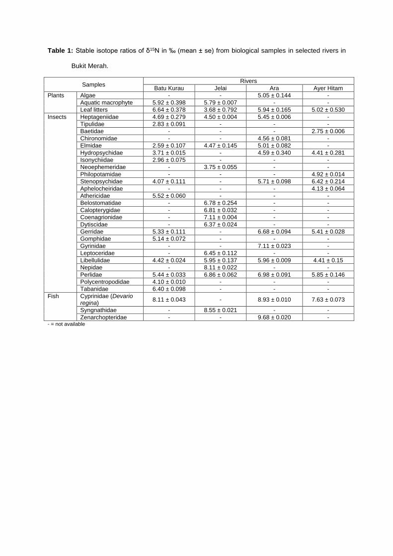
Table 1: Stable isotope ratios of δ15N in ‰ (mean ± se) from biological samples in selected rivers in
Bukit Merah.
Samples Rivers
Batu Kurau Jelai Ara Ayer Hitam
Plants Algae - - 5.05 ± 0.144 -
Aquatic macrophyte 5.92 ± 0.398 5.79 ± 0.007 - -
Leaf litters 6.64 ± 0.378 3.68 ± 0.792 5.94 ± 0.165 5.02 ± 0.530
Insects Heptageniidae 4.69 ± 0.279 4.50 ± 0.004 5.45 ± 0.006 -
Tipulidae 2.83 ± 0.091 - - -
Baetidae - - - 2.75 ± 0.006
Chironomidae - - 4.56 ± 0.081 -
Elmidae 2.59 ± 0.107 4.47 ± 0.145 5.01 ± 0.082 -
Hydropsychidae 3.71 ± 0.015 - 4.59 ± 0.340 4.41 ± 0.281
Isonychiidae 2.96 ± 0.075 - - -
Neoephemeridae - 3.75 ± 0.055 - -
Philopotamidae - - - 4.92 ± 0.014
Stenopsychidae 4.07 ± 0.111 - 5.71 ± 0.098 6.42 ± 0.214
Aphelocheiridae - - - 4.13 ± 0.064
Athericidae 5.52 ± 0.060 - - -
Belostomatidae - 6.78 ± 0.254 - -
Calopterygidae - 6.81 ± 0.032 - -
Coenagrionidae - 7.11 ± 0.004 - -
Dytiscidae - 6.37 ± 0.024 - -
Gerridae 5.33 ± 0.111 - 6.68 ± 0.094 5.41 ± 0.028
Gomphidae 5.14 ± 0.072 - - -
Gyrinidae - - 7.11 ± 0.023 -
Leptoceridae - 6.45 ± 0.112 - -
Libellulidae 4.42 ± 0.024 5.95 ± 0.137 5.96 ± 0.009 4.41 ± 0.15
Nepidae - 8.11 ± 0.022 - -
Perlidae 5.44 ± 0.033 6.86 ± 0.062 6.98 ± 0.091 5.85 ± 0.146
Polycentropodidae 4.10 ± 0.010 - - -
Tabanidae 6.40 ± 0.098 - - -
Fish Cyprinidae (Devario regina)
8.11 ± 0.043 - 8.93 ± 0.010 7.63 ± 0.073
Syngnathidae - 8.55 ± 0.021 - -
Zenarchopteridae - - 9.68 ± 0.020 - - = not available
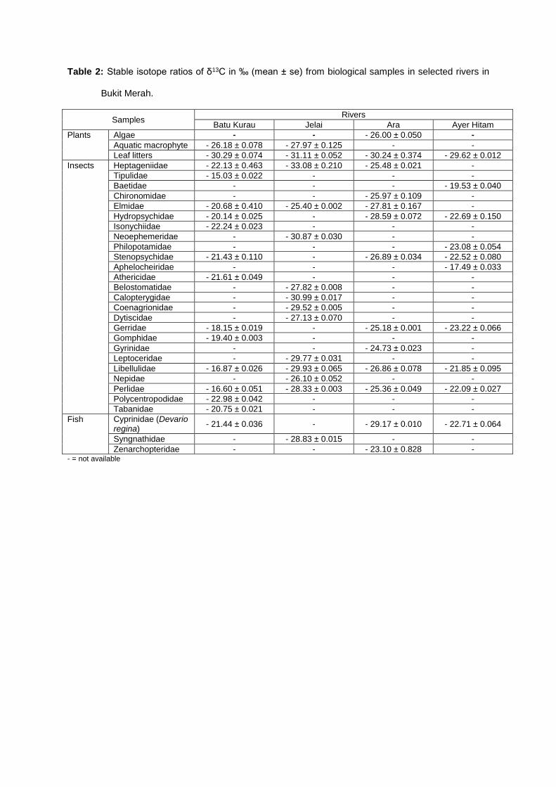
Table 2: Stable isotope ratios of δ13C in ‰ (mean ± se) from biological samples in selected rivers in
Bukit Merah.
Samples Rivers
Batu Kurau Jelai Ara Ayer Hitam
Plants Algae - - - 26.00 ± 0.050 -
Aquatic macrophyte - 26.18 ± 0.078 - 27.97 ± 0.125 - -
Leaf litters - 30.29 ± 0.074 - 31.11 ± 0.052 - 30.24 ± 0.374 - 29.62 ± 0.012
Insects Heptageniidae - 22.13 ± 0.463 - 33.08 ± 0.210 - 25.48 ± 0.021 -
Tipulidae - 15.03 ± 0.022 - - -
Baetidae - - - - 19.53 ± 0.040
Chironomidae - - - 25.97 ± 0.109 -
Elmidae - 20.68 ± 0.410 - 25.40 ± 0.002 - 27.81 ± 0.167 -
Hydropsychidae - 20.14 ± 0.025 - - 28.59 ± 0.072 - 22.69 ± 0.150
Isonychiidae - 22.24 ± 0.023 - - -
Neoephemeridae - - 30.87 ± 0.030 - -
Philopotamidae - - - - 23.08 ± 0.054
Stenopsychidae - 21.43 ± 0.110 - - 26.89 ± 0.034 - 22.52 ± 0.080
Aphelocheiridae - - - - 17.49 ± 0.033
Athericidae - 21.61 ± 0.049 - - -
Belostomatidae - - 27.82 ± 0.008 - -
Calopterygidae - - 30.99 ± 0.017 - -
Coenagrionidae - - 29.52 ± 0.005 - -
Dytiscidae - - 27.13 ± 0.070 - -
Gerridae - 18.15 ± 0.019 - - 25.18 ± 0.001 - 23.22 ± 0.066
Gomphidae - 19.40 ± 0.003 - - -
Gyrinidae - - - 24.73 ± 0.023 -
Leptoceridae - - 29.77 ± 0.031 - -
Libellulidae - 16.87 ± 0.026 - 29.93 ± 0.065 - 26.86 ± 0.078 - 21.85 ± 0.095
Nepidae - - 26.10 ± 0.052 - -
Perlidae - 16.60 ± 0.051 - 28.33 ± 0.003 - 25.36 ± 0.049 - 22.09 ± 0.027
Polycentropodidae - 22.98 ± 0.042 - - -
Tabanidae - 20.75 ± 0.021 - - -
Fish Cyprinidae (Devario regina)
- 21.44 ± 0.036 - - 29.17 ± 0.010 - 22.71 ± 0.064
Syngnathidae - - 28.83 ± 0.015 - -
Zenarchopteridae - - - 23.10 ± 0.828 - - = not available
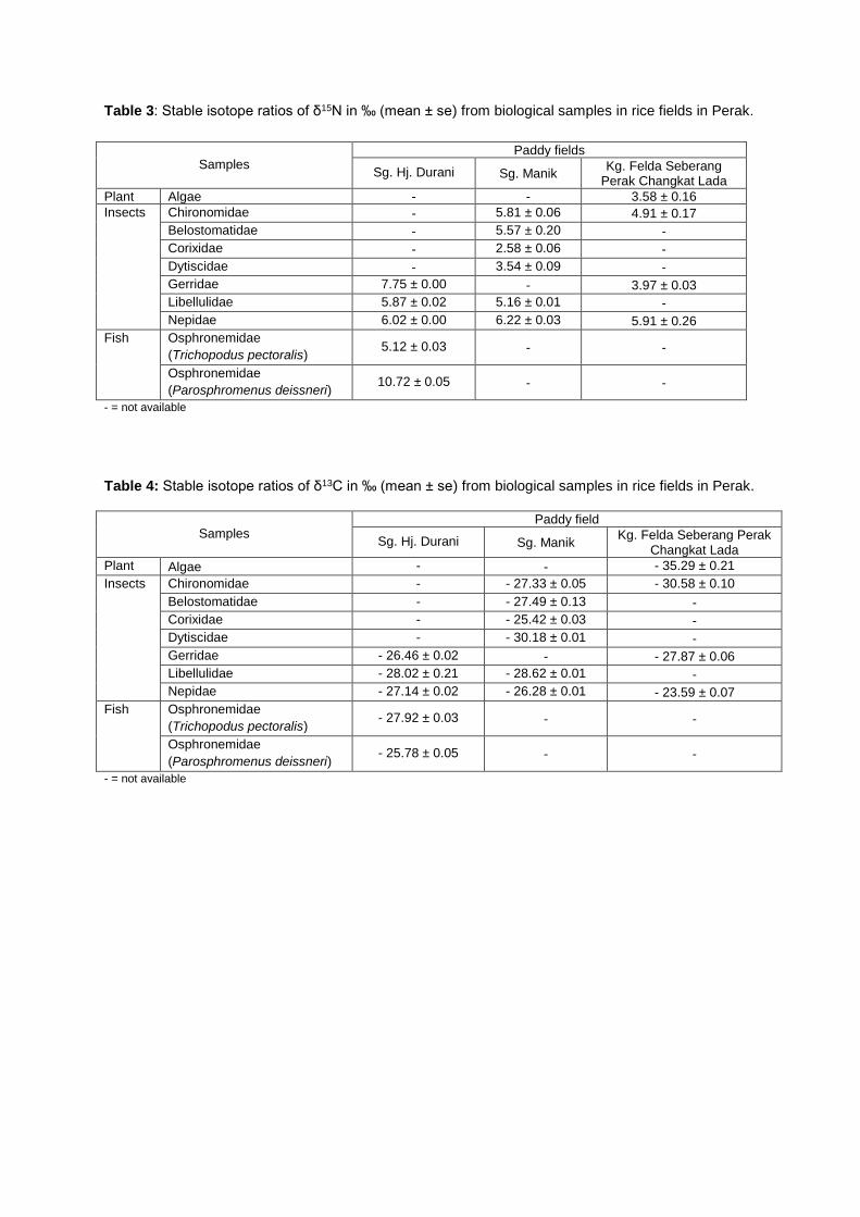
Table 3: Stable isotope ratios of δ15N in ‰ (mean ± se) from biological samples in rice fields in Perak.
Samples Paddy fields
Sg. Hj. Durani Sg. Manik Kg. Felda Seberang
Perak Changkat Lada
Plant Algae - - 3.58 ± 0.16
Insects Chironomidae - 5.81 ± 0.06 4.91 ± 0.17
Belostomatidae - 5.57 ± 0.20 -
Corixidae - 2.58 ± 0.06 -
Dytiscidae - 3.54 ± 0.09 -
Gerridae 7.75 ± 0.00 - 3.97 ± 0.03
Libellulidae 5.87 ± 0.02 5.16 ± 0.01 -
Nepidae 6.02 ± 0.00 6.22 ± 0.03 5.91 ± 0.26
Fish Osphronemidae
(Trichopodus pectoralis) 5.12 ± 0.03 - -
Osphronemidae
(Parosphromenus deissneri) 10.72 ± 0.05 - -
- = not available
Table 4: Stable isotope ratios of δ13C in ‰ (mean ± se) from biological samples in rice fields in Perak.
Samples Paddy field
Sg. Hj. Durani Sg. Manik Kg. Felda Seberang Perak
Changkat Lada
Plant Algae - - - 35.29 ± 0.21
Insects Chironomidae - - 27.33 ± 0.05 - 30.58 ± 0.10
Belostomatidae - - 27.49 ± 0.13 -
Corixidae - - 25.42 ± 0.03 -
Dytiscidae - - 30.18 ± 0.01 -
Gerridae - 26.46 ± 0.02 - - 27.87 ± 0.06
Libellulidae - 28.02 ± 0.21 - 28.62 ± 0.01 -
Nepidae - 27.14 ± 0.02 - 26.28 ± 0.01 - 23.59 ± 0.07
Fish Osphronemidae
(Trichopodus pectoralis) - 27.92 ± 0.03 - -
Osphronemidae
(Parosphromenus deissneri) - 25.78 ± 0.05 - -
- = not available
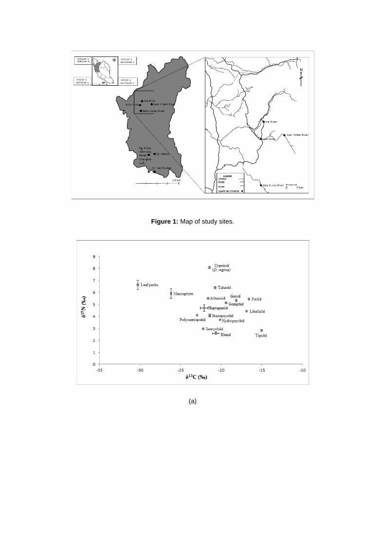
Figure 1: Map of study sites.
(a)
(b)
(c)
(d)
Figure 2: Dual isotopic plots of δ15N and δ13C of plants, aquatic insects and fish from rivers in Perak:
2 (a) Batu Kurau River, 2 (b) Jelai River, 2 (c) Ara River, 2 (d) Ayer Hitam River. Key of
marker shapes: x – producers; circle – primary consumers; diamond – secondary consumers;
triangle – tertiary consumers.
(a)
(b)
(c)
Figure 3: Dual isotopic plots of δ15N and δ13C of plants, aquatic insects and fish from rice fields in
Perak: 3 (a) Sg. Haji Durani, 3 (b) Sg. Manik, 3 (c) Kg. Felda Seberang Perak Changkat Lada.
Key of marker shapes: x – producers; circle – primary consumers; diamond – secondary
consumers; triangle – tertiary consumers.