VOT 79018

DESIGN AND DEVELOPMENT OF FRACTAL ANTENNA FOR ULTRA HIGH FREQUENCY BAND APPLICATION

(MEREKABENTUK DAN MEMBANGUNKAN ANTENA FRACTAL UNTUK APLIKASI JALUR ULTRA

FREKUENSI TINGGI)

MOHAMAD KAMAL A. RAHIM

RESEARCH VOTE NO:

79018

Jabatan Kejuruteraan Perhubungan Radio

Fakulti Kejuruteraan Elektrik Universiti Teknologi Malaysia

2008

Lampiran 20 UTM/RMC/F/0024 (1998)

UNIVERSITI TEKNOLOGI MALAYSIA

BORANG PENGESAHAN LAPORAN AKHIR PENYELIDIKAN

JUDUL: DESIGN AND DEVELOPMENT OF FRACTAL ANTENNA

FOR UHF BAND APPLICATION

Saya MOHAMAD KAMAL A. RAHIM (HURUF BESAR)

mengaku membenarkan Laporan Akhir Penyelidikan ini disimpan di Perpustakaan Universiti Teknologi Malaysia dengan syarat-syarat kegunaan seperti berikut:

1. Tesis adalah hak milik Universiti Teknologi Malaysia.

2. Perpustakaan Universiti Teknologi Malaysia dibenarkan membuat salinan untuk tujuan

pengajian sahaja.

3. Perpustakaan dibenarkan membuat salinan tesis ini sebagai bahan pertukaran antara

institusi pengajian tinggi.

4. *Sila tandakan ( )

(Mengandungi maklumat yang berdarjah keselamatan atau

SULIT kepentingan Malaysia seperti yang termaktub di dalam AKTA RAHSIA RASMI 1972)

TERHAD (Mengandungi maklumat TERHAD yang telah ditentukan oleh organisasi/badan di mana penyelidikan dijalankan)

TIDAK TERHAD

Disahkan oleh,

__________________________________

( TANDATANGAN KETUA PENYELIDIK )

Prof Madya Dr Mohamad Kamal A Rahim

Nama & Cop Ketua Penyelidik

Tarikh : 8 Ogos 2008 CATATAN: * Jika tesis ini SULIT atau TERHAD, sila lampirkan surat daripada pihak berkuasa/organisasi berkenaan dengan menyatakan sekali sebab dan tempoh tesis ini perlu dikelaskan sebagai SULIT atau TERHAD

√

VOT 79018

DESIGN AND DEVELOPMENT OF FRACTAL ANTENNA FOR ULTRA HIGH FREQUENCY BAND APPLICATION

(MEREKABENTUK DAN MEMBANGUNKAN ANTENA FRACTAL UNTUK APLIKASI JALUR ULTRA

FREKUENSI TINGGI)

MOHAMAD KAMAL A. RAHIM

RESEARCH VOTE NO:

79018

Jabatan Kejuruteraan Perhubungan Radio

Fakulti Kejuruteraan Elektrik Universiti Teknologi Malaysia

2008

ii

DECLARATION

I declare that this report entitled “Design and Development of Fractal Antenna for Ultra

High Frequency (UHF) Band Application” is the result of my own research except as

cited in the references.

Signature : .................... ................................

Name of Supervisor : ASSOC. PROF. DR. MOHAMAD KAMAL B.

ABD. RAHIM

Date : OGOS 2008

iii

ACKNOWLEDGEMENT

In finishing this project, I was in contact with many people, researchers,

academicians, and practitioners. They have contributed towards my understanding and

thoughts. In particular, I am also very thankful to Mr. Thelaha, a Ph.D. Student of UTM

and all my fellow researchers for their helps. Without their continued support and

interest, this project would not have been the same as presented here.

I am also indebted to Universiti Teknologi Malaysia (UTM) for funding my

research. Besides, librarians at UTM also deserve special thanks for their assistance in

supplying the relevant literatures.

My fellow researchers should also be recognized for their support. My sincere

appreciation also extends to all my colleagues and others who have provided assistance at

various occasions. Their views and tips are useful indeed. Unfortunately, it is not possible

to list all of them in this limited space. Last but not least, I am truly grateful for having

such a supportive family members.

iv

DESIGN AND DEVELOPMENT OF FRACTAL ANTENNA FOR ULTRA HIGH FREQUENCY BAND APPLICATION

(Keywords: Fractal antenna, Ultra High Frequency)

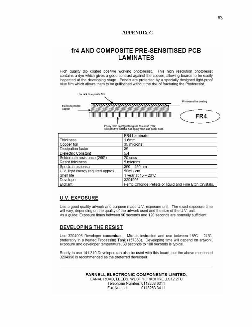
The Ultra High Frequency (UHF) band has long been used for voice, data and

video communication. The lower frequency band of the UHF which is the 470 – 890

MHz is used for terrestrial TV broadcast. The conventional UHF antennas for receiving

TV signals are quite large and directional. It would be better to have a compact and

omnidirectional antenna that can be easily fabricated, especially for portable devices

such as portable televisions. Koch curve fractal structure is one of the fractal geometries

used in antenna designs. One of the benefits of using fractals in the design of antenna

structure includes miniaturization. The dipole antenna is one of the omnidirectional that

can be easily designed. The planar type of antenna is one of the easies t to fabricate. This

project report describes the design of the planar fractal antenna for the uhf band using

the Koch curve structure. Different shapes of antenna using the truncated ground plane

have been designed and simulated to investigate which is the one that gives the best

performance. The simulation process was done using the Agilent ADS software and

Computer Simulation Technology CST. The antenna has been fabricated on the FR4

microstrip board with 7.4=rε and thickness of 1.6 mm using the photolithography and

wet etching technique. The simulation result shows that the Koch curve can be used

to minimize the length of the dipole. It also shows that the folded dipole configuration

together with using Koch curve can increase bandwidth and minimize the length of the

antenna. The fabricated antenna have been test and measured in term of radiation pattern

and return loss and it can be used at a certain band of frequencies.

Key Researcher:

Assoc. Prof. Dr. Mohammad Kamal A. Rahim (Head) Mr Nazri A. Karim Mr. Thelaha Masri Mr Huda A. Majid Mr Osman Ayop

e-mail : mkamal@fke.utm.my Tel No. : 07-5536088 Vote No. : 79018

v

MEREKABENTUK DAN MEMBANGUNKAN ANTENA FRACTAL UNTUK APLIKASI JALUR ULTRA FREKUENSI TINGGI (Kata kunci: Antena Fractal, Ultra Frekuensi Tinggi)

Jalur Ultra Frekuensi Tinggi (UHF) telah lama digunakan untuk komunikasi video,

suara, dan data. Frekuensi jalur rendah daripada UHF iaitu diantara 470–890 MHz

digunakan untuk penyiaran televisyen. Antena UHF yang sekarang banyak digunakan untuk

penerimaan isyarat televisyen adalah agak besar dan terarah. Adalah lebih baik sekiranya

dibuat sebuah antena yang lebih kecil dan semua arah yang dapat dengan mudah dibuat,

terutamanya untuk alatan mudah alih seperti televisyen mudah alih .Struktur fractal

lengkungan Koch adalah salah satu bentuk yang digunakan untuk merekabentuk antena.

Salah satu kelebihan menggunakan fractal adalah mengecilkan saiz struktur. Antena dipole

adalah salah satu antena semua arah yang mudah untuk direkabentuk. Antena jenis

planar adalah salah satu bentuk antena yang paling mudah difabrikasi. Projek ini

menerangkan tentang rekabentuk antena planar fractal untuk jalur UHF menggunakan

struktur Koch. Pelbagai bentuk antena menggunakan satah bumi terpenggal telah

direkabentuk dan disimulasi untuk mengkaji prestasi yang paling bagus. Proses simulasi telah

dilakukan menggunakan perisian Agilent ADS. Antena difabrikasi menggunakan papan

FR4 dengan 7.4=rε dengan ketebalan 1.6 mm menggunakan teknik photolitography dan

punaran basahan. Hasil simulasi menunjukkan bahawa panjang antena dipole boleh

dikurangkan menggunakan lengkungan Koch. Ia juga menunjukkan konfigurasi lipatan

dipole bersama lengkungan Koch boleh meningkatkan lebar jalur dan mengurangkan

panjang antena. Antena yang telah difabrikasi diuji dari segi bentuk penyinaran dan

kehilangan balikan dan boleh digunakan pada sesetengah jalur frekuensi.

Penyelidik:

Assoc. Prof. Dr. Mohammad Kamal A. Rahim (Head) Mr Nazri A. Karim Mr. Thelaha Masri Mr Huda A. Majid Mr Osman Ayop

e-mail : mkamal@fke.utm.my Tel No. : 07-5536088 Vote No. : 79018

vi

TABLE OF CONTENT

CHAPTER TITLE PAGE

TITLE i

DECLARATION ii

ACKNOWLEGMENT iii

ABSTRACT (ENGLISH) iv

ABSTRAK (BAHASA MALAYSIA) v

TABLE OF CONTENTS vi

LIST OF FIGURES ix

LIST OF SYMBOLS xi

LIST OF ABBREVIATIONS xii

1 INTRODUCTION AND BACKGROUND

OF RESEARCH

1.0 Introduction 1

1.1 Problem Statement 4

1.2 Objective 4

1.2 Scope of Project 5

1.3 Organization of Thesis 5

1.4 Summary 6

vii

2 LITERATURE REVIEW

2.1 Introduction 7

2.2 Classification of antennas 7

2.2.1 Frequency and size 7

2.2.2 Directivity 8

2.2.3 Physical construction 8

2.2.4 Application 8

2.3 Antenna Properties 9

2.3.1 Operating Frequency 9

2.3.2 Return Loss 10

2.3.3 Bandwidth 10

2.3.4 Antenna Radiation Patterns 11

2.3.5 Power Gain 11

2.3.6 Directivity 12

2.3.7 Polarization 12

2.4 TV Antenna Basics 13

2.5 Dipole Antenna 15

2.6 Planar Antennas 19

3 FRACTAL DIPOLE ANTENNA DESIGN

3.0 Introduction 21

3.1 Antenna Design Specifications 21

3.2 Design of the antenna using antenna design software 23

3.3 Simulation Using Computer Simulation Technology 27

3.3.1 SMA and Waveguide Port Connector 28

3.3.2 Fundamental Quasi-TEM mode 29

3.4 Simulated Single Koch Dipole 31

3.5 Fabrication of the antenna 33

3.6 Measurements of the Antenna 37

viii

3.6.1 Input Return Loss Measurement 37

3.6.2 Radiation Pattern Measurement 38

3.7 Summary 39

4 RESULTS & DISCUSSIONS

4.0 Introduction 40

4.1 Antenna Simulation Results 40

4.1.1 Standard straight line dipole 40

4.1.2 3rd order Koch curve dipole 42

4.2 Antenna Measurement Results 46

4.2.1 Return Loss Measurement Results 46

4.2.2 Radiation Pattern Measurement Results 49

4.3 Summary 55

5 CONCLUSION

5.0 Conclusion 56

5.1 Proposed Future Work 57

REFERENCES 58

APPENDIX A 61

APPENDIX B 62

APPENDIX C 63

ix

LIST OF FIGURES

FIGURE NO. TITLE PAGE

2.1 Radiation pattern of an antenna 11

2.2 Current (a) and voltage (b) distribution of a half wave dipole 15

2.3 Center feed half wavelength dipole structure 16

2.4 Radiation pattern of the dipole antenna 17

3.1 Circuit schematic of the first order Koch 23

3.2 Circuit design of the second order Koch 24

3.3 The layout of the 3rd

order Koch 24

3.4 Layout of the first design dipole antenna 25

3.5 Layout of the meander lined dipole antenna 26

3.6 Layout of the 3rd

order Koch dipole 26

3.7 Layout of the modified 3rd order Koch 27

3.8 SMA Port 28

3.9 Waveguide port mode 30

3.10 Simulated Koch Dipole Antenna 31

3.11 Dipole Array Antenna 32

3.12 Fractal Koch Dipole Array 32

3.13 Front side photograph of the double sided planar folded dipole 34

3.14 Back side photograph of the double sided planar folded dipole 34

3.15 Front side photograph of the double sided planar modified 3rd order Koch folded dipole 35

3.16 Back side photograph of the double sided planar modified

3rd order Koch folded dipole 35

3.17 Fabricated Koch Dipole Antenna with different flare angle 36

x

3.18 Fabricated Fractal Koch Dipole Array 37

4.1 Simulated return loss of the standard straight line dipole 41

4.2 Simulated return loss of the meandered line dipole 42

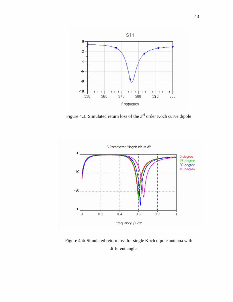
4.3 Simulated return loss of the 3rd order Koch curve dipole 43

4.4 Simulated return loss for single Koch dipole antenna

with different angle. 43

4.5 3D Radiation Pattern with different flare angle 44

4.6 Simulated return loss for Fractal Koch Dipole Array 45

4.7 3D simulated radiation pattern for Fractal Koch Dipole Array 45

4.8 Measurement and simulation result for folded straight dipole 47

4.9 Measurement and simulation result of the folded modified Koch

dipole 48

4.10 Measurement and simulation return loss of fractal Koch

dipole array 49

4.11 Measured radiation pattern for the E-Co and E-Cross of the folded

straight dipole. 50

4.12 Measured radiation pattern for the H-Co of the folded

Koch antenna 51

4.13 Measurement result for E-Co and E Cross of the folded

Koch dipole 52

4.14 Measurement results for the H-Co radiation pattern of the folded

Koch dipole 52

4.15 Measured radiation pattern for E-Plane of the fractal Koch dipole

array 53

4.16 Measured radiation pattern for H- Plane of the fractal Koch dipole

array 54

4.17 Measured Co & Cross Polar of the fractal Koch dipole array 54

xi

LIST OF SYMBOLS

dB - decibel

W - Width of rectangular patch antenna

L - Length of rectangular patch antenna

εr - Dielectric constant

h - Substrate height

λg - Guided wavelength

fu - Upper cutoff frequency

fl - Lower cutoff frequency

d - distance between antenna elements

θ - phase

k - wave number

λ0 - wavelength in free space

l - transmission line length

Zo - characteristic impedance

w - transmission line width

εeff - effective dielectric constant

c - velocity of light in free space

fr - operating frequency

BW% - bandwidth in percentage

xii

LIST OF ABBREVIATIONS

UHF - Ultra High Frequency

VHF - Very High Frequency

WLAN - Wireless Local Area Network

CHAPTER 1

INTRODUCTION

1.1 Introduction

During the past ten years, the mobile radio communications industry has

grown by orders of magnitude, fuelled by digital and RF circuit fabrication

improvements, new large -scale circuit integration, and other miniaturization

technologies which make portable radio equipment smaller, cheaper, and more

reliable. These trends will continue at an even greater pace during the next decade.

Wireless operations, such as long range communications, are impossible or

impractical to implement with the use of wires. The term is commonly used in the

telecommunications industry to refer to telecommunications systems (e.g., radio

transmitters and receivers, remote controls, computer networks, network terminals,

etc.) which use some form of energy (e.g.,radio frequency (RF), infrared light,

laser light, visible light, acoustic energy, etc.) to transfer information without the

use of wires. Information is transferred in this manner over both short and long

distances. Applications may involve point-to-point ommunication, point-to-multipoint

communication, broadcasting, cellular networks and other wireless networks.

2

Antenna is a very important component for the wireless communication

systems using radio frequency and microwaves. By definition, an antenna is a

device used to transform an RF signal, traveling on a conductor, into an

electromagnetic wave in free space. The IEEE Standard Definitions of Terms for

Antennas (IEEE Std 145-1983) defines the antenna or aerial as “a means for

radiating or receiving radio waves”. In other words it is a transitional structure

between free space and a guiding device that is made to efficiently radiate and

receive radiated electromagnetic waves. Antennas are commonly used in radio,

television broadcasting, cell phones, radar and other systems involving the use of

electromagnetic waves. Antennas demonstrate a property known as reciprocity, which

means that an antenna will maintain the same characteristics regardless if it is

transmitting or receiving.

One of the applications of a one way wireless communication is the

terrestrial television. Terrestrial television (also known as over-the-air, OTA or

broadcast television) is the method of television broadcast signal (can be analog or

digital) delivery by using radio waves from broadcast stations to televisions at

homes using air as the medium. In terrestrial TV system, the transmitters (broadcast

stations) are transmitting the TV signal with high power and very tall antenna

transmitters located on the ground to transmit radio waves to the surrounding area.

Viewers can pick up the signal with a much smaller antenna. The main limitation of

broadcast television is range. The frequency r a n g e used by the terrestrial

television includes the very high frequency (VHF) and ultra high frequency

(UHF). The most common antenna used for receiving TV signals are the the Yagi-

Uda antenna (variation of the dipole antenna) which is traditionally placed on the

roof of the house.

One of the other types of the antenna is the planar antenna. The planar antenna has

the most variation compared to any other types of antenna. Due to its advantages such

3

as low profile and the capability to be fabricated using the printed circuit technology,

antenna manufacturers and researchers can come out with a novel design of antenna

in house which will reduce the cost of its development. Planar antennas are also

relatively inexpensive to manufacture and design because of the simple 2-dimensional

physical geometry. They are usually employed at UHF and higher frequencies

because the size of the antenna is directly tied to the wavelength at the resonant

frequency.

Fractal geometries have been applied to antenna design to make multiband

and broadband antennas. In addition, fractal geometries have been used to

miniaturise the size of the antennas. However, miniaturization has been mostly limited

to the wire (dipole and loop) antennas. The geometry of the fractal antenna

encourages its study both as a multiband solution and also as a small (physical size)

antenna. First, because one should expect a selfsimilar antenna (which contains

many copies of itself at several scales) to operate in a similar way at several

wavelengths. That is, the antenna should keep similar radiation parameters through

several bands. Second, because the space- filling properties of some fractal shapes

(the fractal dimension) might allow fractal shaped small antennas to better take

advantage of the small surrounding space. The fractal antenna is formed by

applying a generator shape repetitively at a constant scale factor and results in an

antenna with log-periodic characteristics which is a multiband antenna and a

miniaturization characteristic.

4

1.2 Problem Statement

Antenna elements are based on the size of the waves they're designed to

receive, and the lower the frequency, the waves are longer, requiring a larger antenna

surface to receive them. UHF TV antenna is significantly large and are intended for

roof- or attic- mounting. The use of big outdoor UHF antenna should be replaced with a

compact, less expensive and easily manufactured dipole antenna. The fractal geometry

combined with the planar dipole can produce an antenna that has the benefit of being

compact, low cost, and easily fabricated. The UHF band spanning from 470 MHz -

890 MHz is used for terrestrial TV broadcast. It will be very useful if the planar fractal

antenna can be utilised in this frequency band.

1.3 Objectives

The objectives of this project are as follows:

To design, simulate and fabricate planar dipole antenna based on the Koch

curve fractal geometry that has operating frequency within the lower UHF band i.e.

470MHz-890MHz which is the terrestrial TV signal frequency band.

5

1.4 Scope of Project

(i) Design the antenna based on previous similar works in published

journals using antenna design software ,

(ii) Simulate the proposed antenna using antenna design software (Agilent

Advanced Design Systems and Computer Simulation Technology CST),

(iii) Fabricate the antenna using the available materials (FR-4 Board).

1.5 Organisation of Project Report

This project report consists of five chapters describing all the work done in the

project. The project report organization is generally described as follows.

The first chapter explain the introduction of the project and problem this

project try to solve which describe the motivation of this project. This chapter sets

the work flows according to the objectives and scope of project.

Chapter two discuss the types of antennas, theories of planar and microstrip

antenna, dipole configuration, and the fractal structure for antennas. Also the

equation needed to design the planar dipole antenna is discussed.

Chapter three discuss the steps on designing the planar fractal dipole antenna,

6

the software used for design and simulation, the structure of the designed antennas,

and the measurement techniques.

Result and analysis are presented in chapter four to compare the performance

of all the designed antennas.

The last chapter highlights the overall conclusion of the project with future

work suggestion to improve the design of the antenna. The project is

summarized in this chapter to give general achievements and the future

improvements can be made by other researchers in the future.

1.6 Summary

This is an introductory chapter that defines the literature review, the

objectives, and research background of the thesis. The project report structure is

explained and highlighted. In the following chapters, the project work performed is

reported.

7

CHAPTER 2

LITERATURE REVIEW

2.1 Introduction

An antenna or aerial is a transducer designed to transmit or receive radio

waves which are a class of electromagnetic waves. In other words, antennas

convert radio frequency electrical currents into electromagnetic waves and vice

versa. Antennas are used in systems such as radio and television broadcasting,

point-to-point radio communication, wireless LAN, radar, and space exploration.

Antennas usually work in air or outer space, but can also be operated under

water or even through soil and rock at certain frequencies for short distances.

2.2 Classification of antennas

2.2.1 Frequency and size

Antennas used for UHF are different from the ones used for VHF, which

in turn are different from antennas for microwave. The wavelength is different

at different frequencies, so the antennas must be different in size to radiate

signals at the correct wavelength.

8

2.2.2 Directivity

Antennas can be omnidirectional, sectorial or directive. Omnidirectional

antennas radiate the same pattern all around the antenna in a complete 360

degrees pattern. The most popular types of omnidirectional antennas are the

Dipole-Type and the Ground Plane. Sectorial antennas radiate primarily in a

specific area. The beam can be as wide as 180 degrees, or as narrow as 60

degrees. Directive antennas are antennas in which the beamwidth is much

narrower than in sectorial antennas. They have the highest gain and are

therefore used for long distance links. Types of directive antennas are the Yagi,

the biquad, the horn, the helicoidal, the patch antenna, the Parabolic Dish and

many others.

2.2.3 Physical construction

Antennas can be constructed in many different ways, ranging from simple

wires to parabolic dishes, up to coffee cans. From the ones that are shaped like

parabola, like fish bones, until the smallest and compact antenna like the ones

printed on PCB.

2.2.4 Application

Two application categories which are Base Station and Point-to-Point.

Each of these suggests different types of antennas for their purpose. Base

Stations are used for multipoint access. Two choices are Omni antennas which

radiate equally in all directions, or Sectorial antennas,which focus into a small

9

area. In the Point-to-Point case, antennas are used to connect two single

locations together. Directive antennas are the primary choice for this application.

All antennas radiate some energy in all directions in free space but careful

construction results in substantial transmission of energy in a preferred

direction and negligible energy radiated in other directions.

2.3 Antenna Properties

There are several important antenna characteristics that should be

considered when choosing an antenna for your application as follows:

2.3.1 Operating frequency

The operating frequency is the frequency range through which the

antenna will meet all functional specifications. It depends on the structure of

the antenna in which each antenna types has its own characteristic towards a

certain range of frequency. The operating frequency can be tuned by adjusting the

electrical length of the antenna.

10

2.3.2 Return Loss

Return loss is the ratio, at the junction of a transmission line and a

terminating impedance or other discontinuity, of the amplitude of the reflected

wave to the amplitude of the incident wave. The return loss value describes

the reduction in the amplitude of the reflected energy, as compared to the forward

energy. Return loss can be expresses as equation 1.

21

2120ZZZZLogRL

−+

= (1)

where : Z1 = impedance toward the source Z2 = impedance toward the load

2.3.3 Bandwidth

Bandwidth can be defined as “the range of frequencies within which the

performance of the antenna, with respect to some characteristics, conform to a

specified standard”. Bandwidth is a measure of frequency range and is

typically measured in hertz. For an antenna that has a frequency range, the

bandwidth is usually expressed in ratio of the upper frequency to the lower

frequency where they coincide with the -10 dB return loss value. The formula for

calculating bandwidth is given in Equation (2).

%100% xffff

BWlh

lh −=

where : fh = lower frequency that coincide with the -10 dB return loss value

fl = upper frequency that coincide with the -10 dB return loss value

11

2.3.4 Antenna radiation patterns

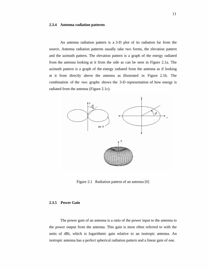
An antenna radiation pattern is a 3-D plot of its radiation far from the

source. Antenna radiation patterns usually take two forms, the elevation pattern

and the azimuth pattern. The elevation pattern is a graph of the energy radiated

from the antenna looking at it from the side as can be seen in Figure 2.1a. The

azimuth pattern is a graph of the energy radiated from the antenna as if looking

at it from directly above the antenna as illustrated in Figure 2.1b. The

combination of the two graphs shows the 3-D representation of how energy is

radiated from the antenna (Figure 2.1c).

Figure 2.1 Radiation pattern of an antenna [6]

2.3.5 Power Gain

The power gain of an antenna is a ratio of the power input to the antenna to

the power output from the antenna. This gain is most often referred to with the

units of dBi, which is logarithmic gain relative to an isotropic antenna. An

isotropic antenna has a perfect spherical radiation pattern and a linear gain of one.

12

?2.3.6 Directivity

The directive gain of an antenna is a measure of the concentration of the

radiated power in a particular direction. It may be regarded as the ability of the

antenna to direct radiated power in a given direction. It is usually a ratio of

radiation intensity in a given direction to the average radiation intensity.

2.3.7 Polarization

Polarization is the orientation of electromagnetic waves far from the

source. There are two fields that will radiate from the antenna, the electrical

field and the magnetic field. Polarization of the antenna or the orientation of

the electric filed (E- plane) of the radio wave is determined by physical

structure of the antenna and its orientation with respect to the surface of the

earth.

There are several types of polarization that apply to antennas. They are

linear, which comprises, vertical, horizontal, and circular polarization is most

important to get the maximum performance from the antennas. For linear

polarization, the antenna radiates the electric field of the emitted radio wave

to a particular orientation. For circular polarization, the antenna continuously

varies the electric field of the radio wave through all possible values of its

orientation with respect to the earth’s surface. For best performance matching up

the polarization of the transmitting antenna and the receiving antenna needs to be

done.

13

2.4 TV Antenna Basics

There is no one antenna or antenna type that will deliver excellent TV

reception in every location. The main factors determining reception are the

distance and direction from the TV station transmitters to your home. Other

factors include the transmitter's power and the height of its tower, the terrain

between the tower and your antenna, and the size and location of any large

buildings in the path of the transmission.

If the receiver is a few kilometres from the transmitter, and the signal

path is relatively unobstructed, you may be able to get adequate reception using a

small set-top indoor antenna. But as you move farther away, getting usable

signal strength becomes trickier. This is where careful antenna selection and

installation become essential.

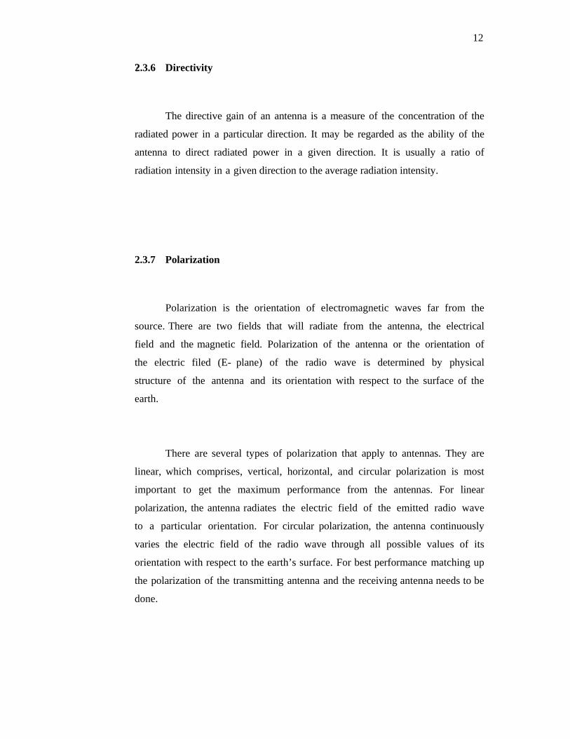
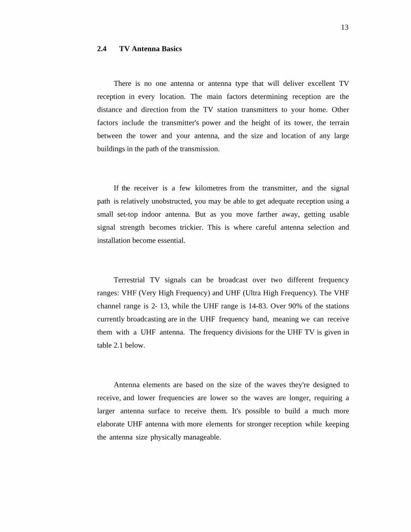
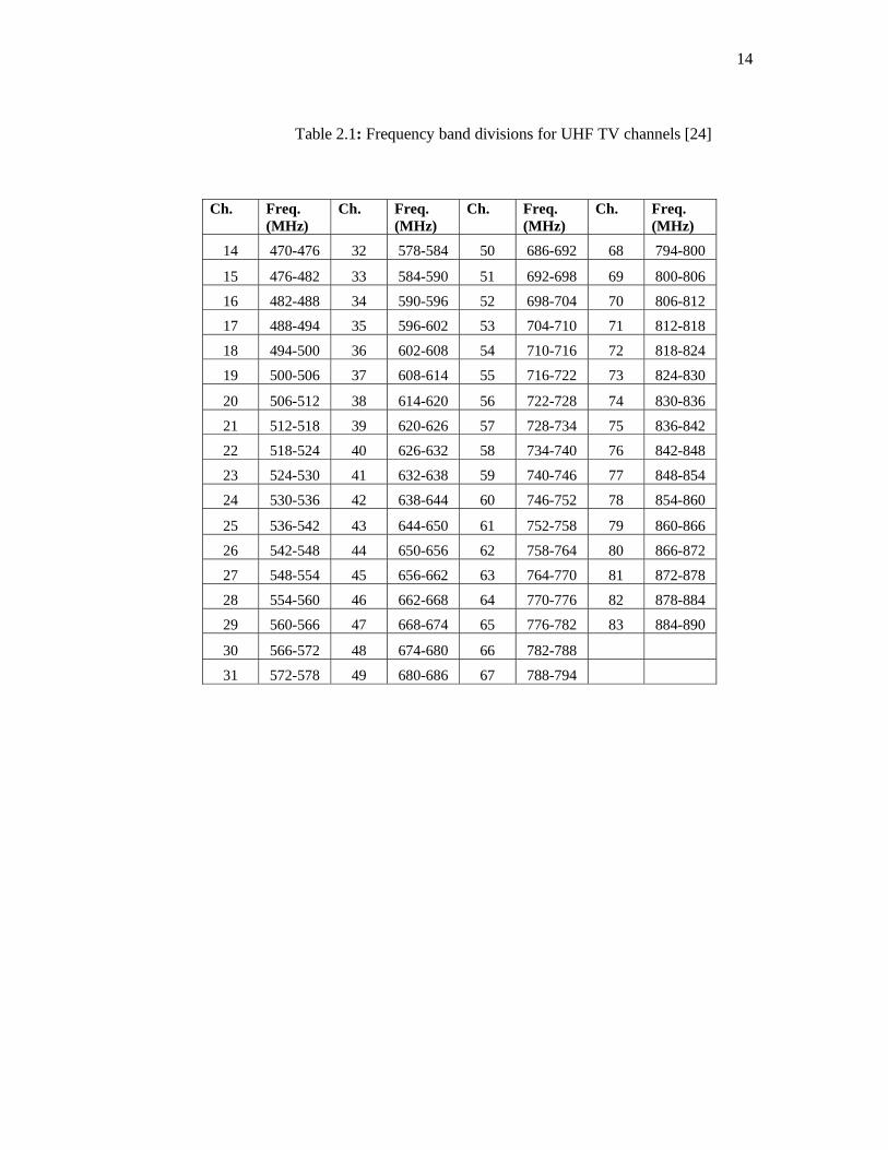
Terrestrial TV signals can be broadcast over two different frequency

ranges: VHF (Very High Frequency) and UHF (Ultra High Frequency). The VHF

channel range is 2- 13, while the UHF range is 14-83. Over 90% of the stations

currently broadcasting are in the UHF frequency band, meaning we can receive

them with a UHF antenna. The frequency divisions for the UHF TV is given in

table 2.1 below.

Antenna elements are based on the size of the waves they're designed to

receive, and lower frequencies are lower so the waves are longer, requiring a

larger antenna surface to receive them. It's possible to build a much more

elaborate UHF antenna with more elements for stronger reception while keeping

the antenna size physically manageable.

14

Table 2.1: Frequency band divisions for UHF TV channels [24]

Ch. Freq. (MHz)

Ch. Freq. (MHz)

Ch. Freq. (MHz)

Ch. Freq. (MHz)

14 470-476 32 578-584 50 686-692 68 794-800

15 476-482 33 584-590 51 692-698 69 800-806

16 482-488 34 590-596 52 698-704 70 806-812

17 488-494 35 596-602 53 704-710 71 812-818

18 494-500 36 602-608 54 710-716 72 818-824

19 500-506 37 608-614 55 716-722 73 824-830

20 506-512 38 614-620 56 722-728 74 830-836

21 512-518 39 620-626 57 728-734 75 836-842

22 518-524 40 626-632 58 734-740 76 842-848

23 524-530 41 632-638 59 740-746 77 848-854

24 530-536 42 638-644 60 746-752 78 854-860

25 536-542 43 644-650 61 752-758 79 860-866

26 542-548 44 650-656 62 758-764 80 866-872

27 548-554 45 656-662 63 764-770 81 872-878

28 554-560 46 662-668 64 770-776 82 878-884

29 560-566 47 668-674 65 776-782 83 884-890

30 566-572 48 674-680 66 782-788

31 572-578 49 680-686 67 788-794

15

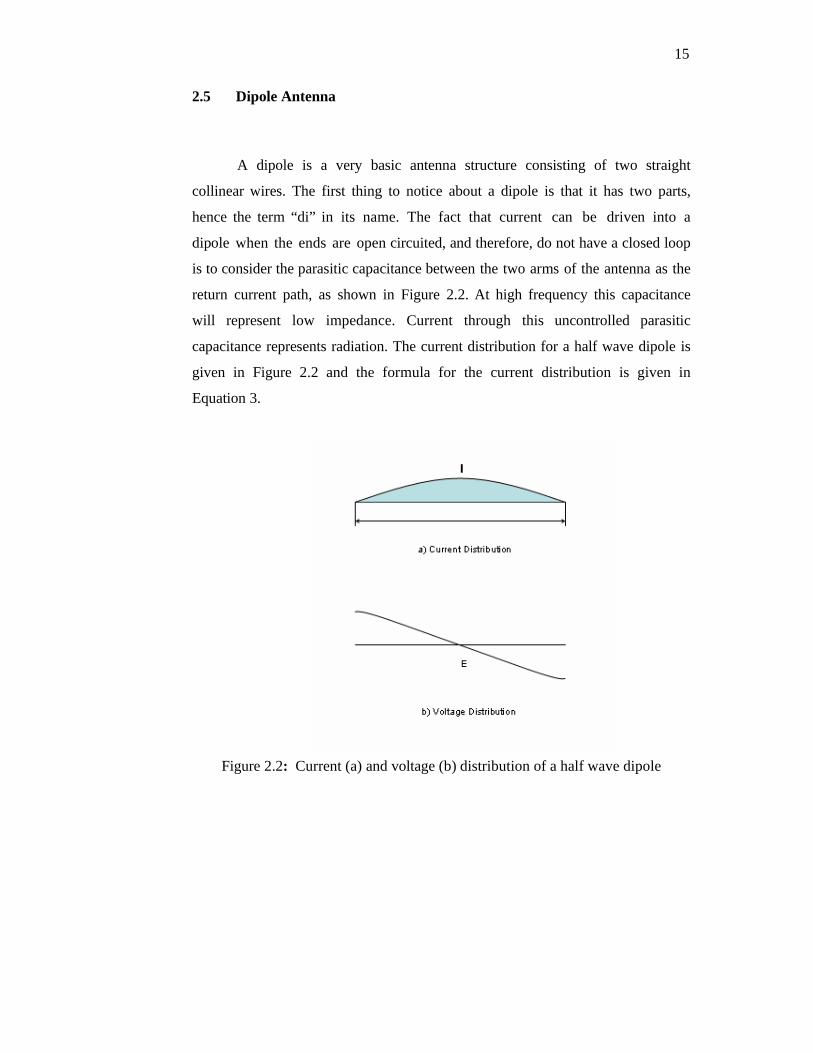
2.5 Dipole Antenna

A dipole is a very basic antenna structure consisting of two straight

collinear wires. The first thing to notice about a dipole is that it has two parts,

hence the term “di” in its name. The fact that current can be driven into a

dipole when the ends are open circuited, and therefore, do not have a closed loop

is to consider the parasitic capacitance between the two arms of the antenna as the

return current path, as shown in Figure 2.2. At high frequency this capacitance

will represent low impedance. Current through this uncontrolled parasitic

capacitance represents radiation. The current distribution for a half wave dipole is

given in Figure 2.2 and the formula for the current distribution is given in

Equation 3.

Figure 2.2: Current (a) and voltage (b) distribution of a half wave dipole

16

lkeII tjo cosϖ= ,

λπ2

=k (3)

where : Io = input current (A) l = each dipole arm length (m)

λ = wavelength (m)

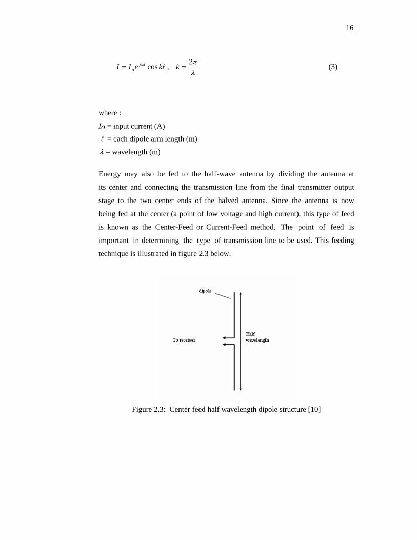
Energy may also be fed to the half-wave antenna by dividing the antenna at

its center and connecting the transmission line from the final transmitter output

stage to the two center ends of the halved antenna. Since the antenna is now

being fed at the center (a point of low voltage and high current), this type of feed

is known as the Center-Feed or Current-Feed method. The point of feed is

important in determining the type of transmission line to be used. This feeding

technique is illustrated in figure 2.3 below.

Figure 2.3: Center feed half wavelength dipole structure [10]

17

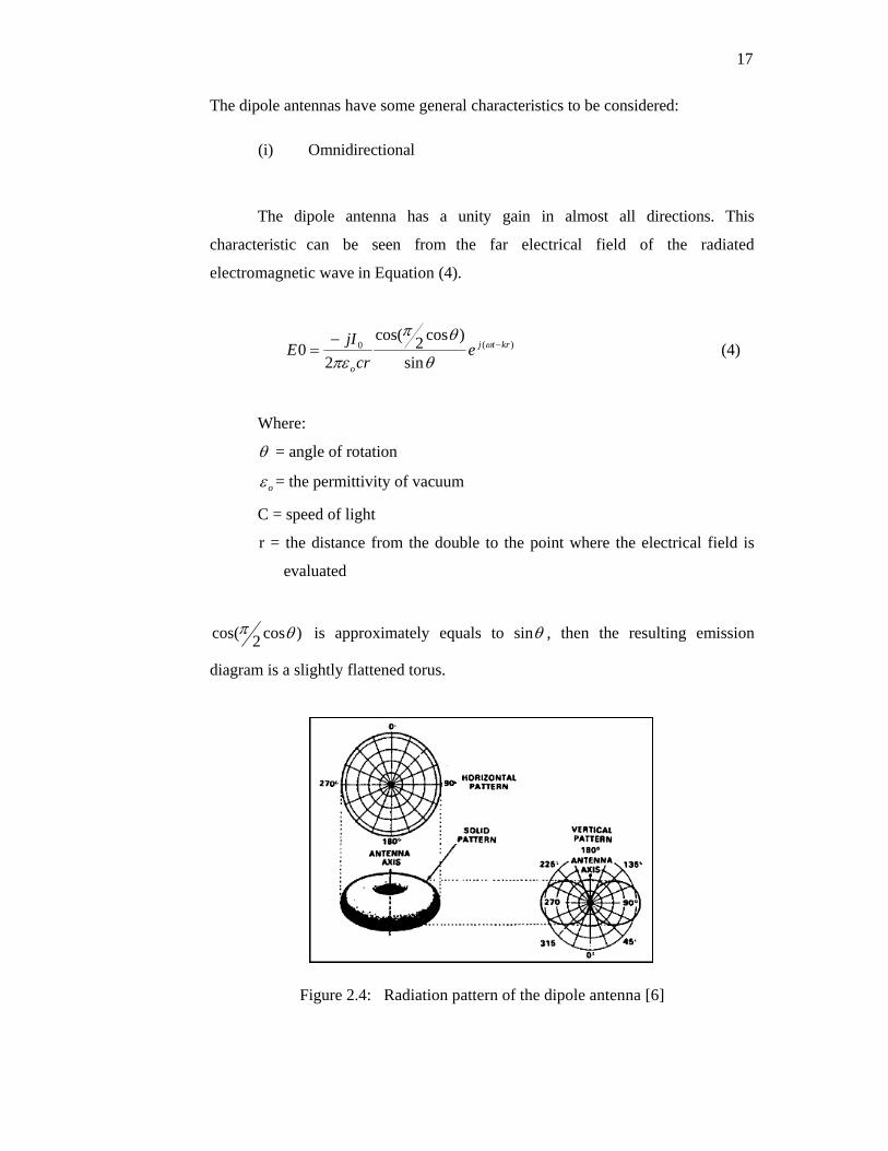
The dipole antennas have some general characteristics to be considered: (i) Omnidirectional

The dipole antenna has a unity gain in almost all directions. This

characteristic can be seen from the far electrical field of the radiated

electromagnetic wave in Equation (4).

)(0

sin

)cos2cos(

20 krtj

o

ecr

jIE −−

= ω

θ

θπ

πε (4)

Where:

θ = angle of rotation

oε = the permittivity of vacuum

C = speed of light

r = the distance from the double to the point where the electrical field is

evaluated

)cos2cos( θπ is approximately equals to sinθ , then the resulting emission

diagram is a slightly flattened torus.

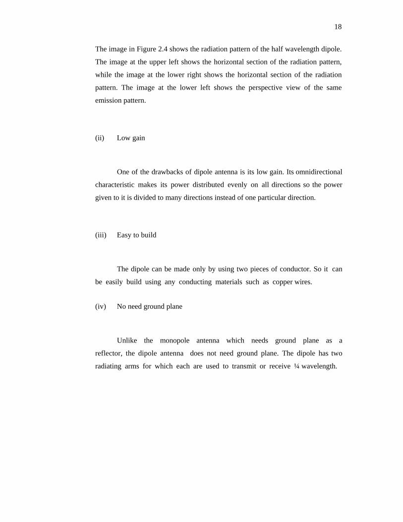
Figure 2.4: Radiation pattern of the dipole antenna [6]

18

The image in Figure 2.4 shows the radiation pattern of the half wavelength dipole.

The image at the upper left shows the horizontal section of the radiation pattern,

while the image at the lower right shows the horizontal section of the radiation

pattern. The image at the lower left shows the perspective view of the same

emission pattern.

(ii) Low gain

One of the drawbacks of dipole antenna is its low gain. Its omnidirectional

characteristic makes its power distributed evenly on all directions so the power

given to it is divided to many directions instead of one particular direction.

(iii) Easy to build

The dipole can be made only by using two pieces of conductor. So it can

be easily build using any conducting materials such as copper wires.

(iv) No need ground plane

Unlike the monopole antenna which needs ground plane as a

reflector, the dipole antenna does not need ground plane. The dipole has two

radiating arms for which each are used to transmit or receive ¼ wavelength.

19

2.6 Planar Antennas

Basically, a planar antenna is an antenna that has a two dimensional

structure. It is usually build over a flat single layer PCB. Planar antennas are very

popular because of their ease of fabrication. If the antenna is to be implemented

on the same PCB as the circuitry, practically no additional costs arise. Planar

antennas are also relatively inexpensive to manufacture and design because of

the simple 2-dimensional physical geometry. They are usually employed at UHF

and higher frequencies because the size of the antenna is directly tied to the

wavelength at the resonant frequency.

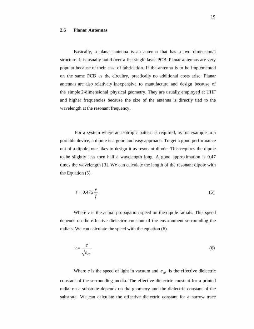
For a system where an isotropic pattern is required, as for example in a

portable device, a dipole is a good and easy approach. To get a good performance

out of a dipole, one likes to design it as resonant dipole. This requires the dipole

to be slightly less then half a wavelength long. A good approximation is 0.47

times the wavelength [3]. We can calculate the length of the resonant dipole with

the Equation (5).

fvx47.0=l (5)

Where v is the actual propagation speed on the dipole radials. This speed

depends on the effective dielectric constant of the environment surrounding the

radials. We can calculate the speed with the equation (6).

eff

cvε

= (6)

Where c is the speed of light in vacuum and effε is the effective dielectric

constant of the surrounding media. The effective dielectric constant for a printed

radial on a substrate depends on the geometry and the dielectric constant of the

substrate. We can calculate the effective dielectric constant for a narrow trace

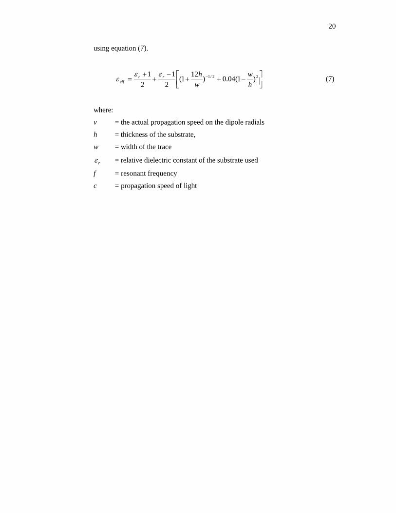
20

using equation (7).

⎥⎦⎤

⎢⎣⎡ −++

−+

+= − 22/1 )1(04.0)121(

21

21

hw

whrr

effεε

ε (7)

where: v = the actual propagation speed on the dipole radials h = thickness of the substrate, w = width of the trace

rε = relative dielectric constant of the substrate used f = resonant frequency c = propagation speed of light

CHAPTER 3

FRACTAL DIPOLE ANTENNA DESIGN

3.0 Introduction

The design of the planar fractal antenna started by choosing the fractal

structure suitable for this type of antenna. The choice is based on theories of fractals and

results from published journals about fractal antennas.

3.1 Antenna Design Specifications

The antenna designed for this project should have the following specifications:

(a) Planar antenna

Antenna is built on a flat surface double layer PCB (copper layered).

(b) Operating at the lower frequency of the UHF band (470-890MHz)

The frequency band 470-890 MHz is chosen because it is the band that is used

for terrestrial UHF TV channels and for new applications like a Digital TV Broadcasting.

22

(c) Dipole antenna

Dipole is chosen because it has the omnidirectional radiation pattern so it cans

receive TV signals no matter which side the antenna is facing.

(d) Koch curve fractal geometry

The Koch curve fractal structure is chosen because of it’s

miniaturization characteristic.

(e) Uses FR4 substrate.

The PCB that is used is the FR4 (Fire Retardant – 4) type board. The reasons

for choosing this type of board are because of the low cost and ease of fabrication. The

FR-4 board has a relative dielectric constant of 7.4=rε with tangent loss of 0.019; it

has a 1.6 mm substrate thickness and a 0.035 mm copper thickness.

(f) Antenna is used to receive signals.

Antenna is receive only because terrestrial TV is broadcast one way

communication which does not need any reply or acknowledgments signals from the

receiver side.

23

3.2 Design of the antenna using antenna design software

There are various software in the market that can be used to design the antenna

or RF component for example Computer Simulation Technology, Advance Design

System ADS, HFSS, Applied Wave Research AWR and many more. In this design,

three software have been used to design the antenna. The design of the antenna is

divided into 2 steps. The first one is designing the antenna structure using circuit in the

schematic feature of the AWR Microwave Office. This step is taken only for the Koch

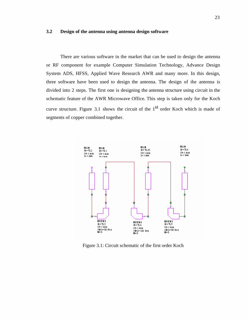
curve structure. Figure 3.1 shows the circuit of the 1st order Koch which is made of

segments of copper combined together.

Figure 3.1: Circuit schematic of the first order Koch

24

Figure 3.2 shows the circuit of the 2nd order Koch which is made out of the

1st order Koch circuits combined.

Figure 3.2: Circuit design of the second order Koch

Figure 3.3 shows the layout of the 3rd order Koch which is made out of the 2nd

order Koch circuits in figure 3.2 combined.

Figure 3.3 : The layout of the 3rd order Koch

This step is taken only for the Koch curve structure, because the Agilent

ADS software does not have the feature to make Koch curve in it’s schematic. After

designing the circuit, the layout is generated. After that, the layout is exported in

GDSII format. Then in ADS software, the GDSII file is imported and rebuilds the

layout in its layout window.

25

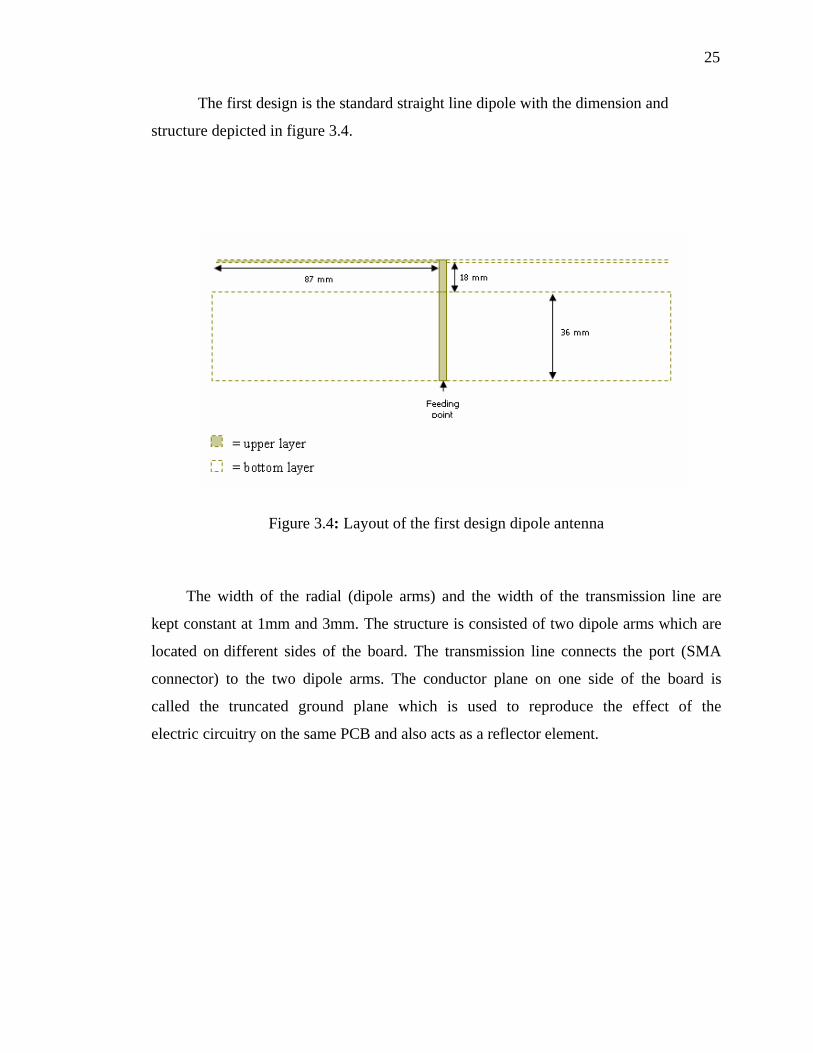
The first design is the standard straight line dipole with the dimension and

structure depicted in figure 3.4.

Figure 3.4: Layout of the first design dipole antenna

The width of the radial (dipole arms) and the width of the transmission line are

kept constant at 1mm and 3mm. The structure is consisted of two dipole arms which are

located on different sides of the board. The transmission line connects the port (SMA

connector) to the two dipole arms. The conductor plane on one side of the board is

called the truncated ground plane which is used to reproduce the effect of the

electric circuitry on the same PCB and also acts as a reflector element.

26

The second design is the modified dipole called meandered dipole with the

dimension and structure depicted in Figure 3.5.

Figure 3.5: Layout of the meander lined dipole antenna

The third design is the 3rd order Koch dipole with the dimension and structure

depicted in figure 3.6.

Figure 3.6: Layout of the 3rd order Koch dipole

27

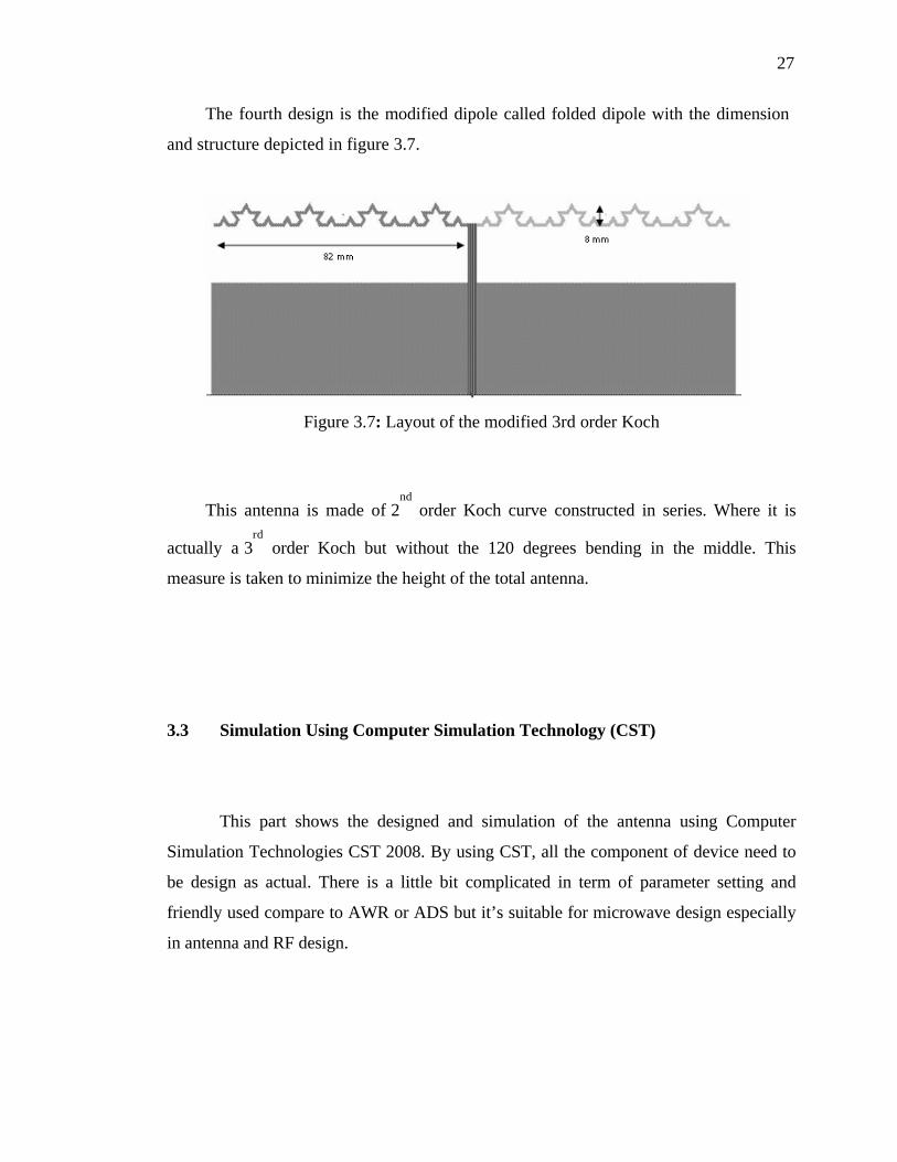
The fourth design is the modified dipole called folded dipole with the dimension

and structure depicted in figure 3.7.

Figure 3.7: Layout of the modified 3rd order Koch

This antenna is made of 2nd

order Koch curve constructed in series. Where it is

actually a 3rd

order Koch but without the 120 degrees bending in the middle. This

measure is taken to minimize the height of the total antenna.

3.3 Simulation Using Computer Simulation Technology (CST)

This part shows the designed and simulation of the antenna using Computer

Simulation Technologies CST 2008. By using CST, all the component of device need to

be design as actual. There is a little bit complicated in term of parameter setting and

friendly used compare to AWR or ADS but it’s suitable for microwave design especially

in antenna and RF design.

28

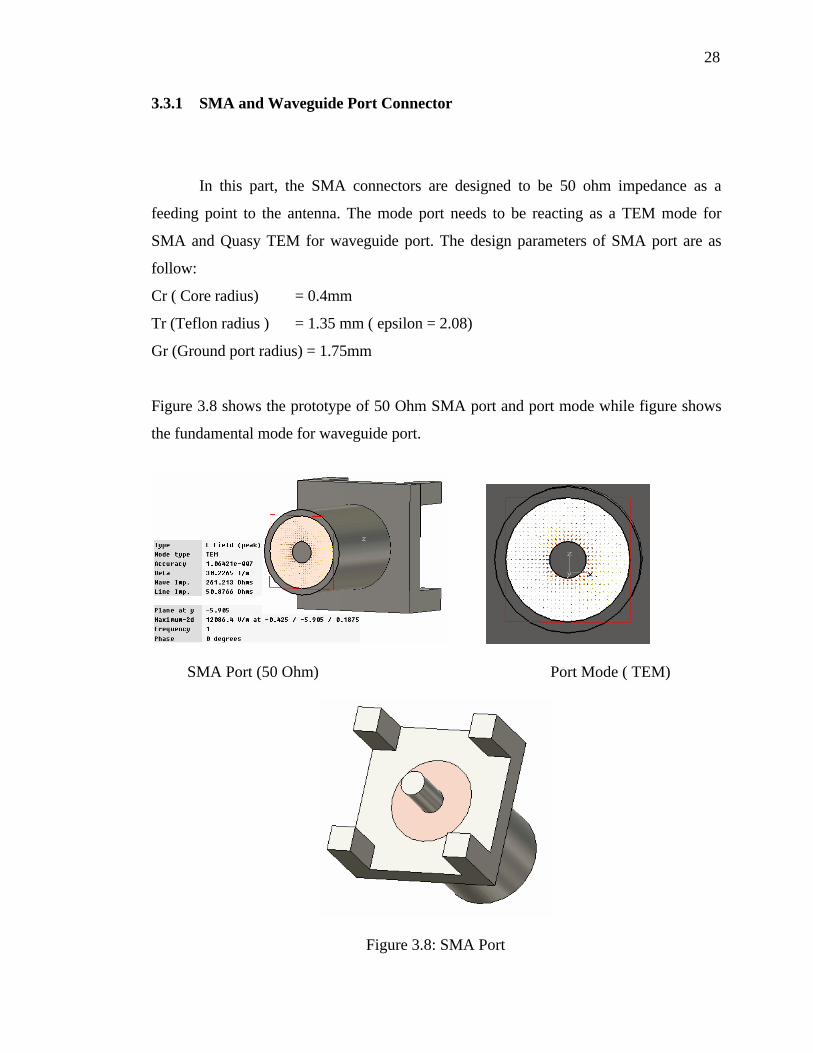
3.3.1 SMA and Waveguide Port Connector

In this part, the SMA connectors are designed to be 50 ohm impedance as a

feeding point to the antenna. The mode port needs to be reacting as a TEM mode for

SMA and Quasy TEM for waveguide port. The design parameters of SMA port are as

follow:

Cr ( Core radius) = 0.4mm

Tr (Teflon radius ) = 1.35 mm ( epsilon = 2.08)

Gr (Ground port radius) = 1.75mm

Figure 3.8 shows the prototype of 50 Ohm SMA port and port mode while figure shows

the fundamental mode for waveguide port.

SMA Port (50 Ohm) Port Mode ( TEM)

Figure 3.8: SMA Port

29

3.3.2 Fundamental Quasi-TEM mode

In general, the size of the port is a very important consideration. On one hand,

the port needs to be large enough to enclose the significant part of the microstrip line’s

fundamental quasi-TEM mode. On the other hand, the port size should not be chosen

unnecessarily large because this may cause higher order waveguide modes to propagate

in the port.

The following pictures show the fundamental microstrip line mode and higher

order mode.

Fundamental mode Higher order mode

a) Port mode

The higher order modes of the microstrip line are very similar to modes in rectangular

waveguides. This behavior can be explained by an enclosure that is automatically added

along the port’s circumference for the port mode calculation. The boundary conditions at

the port’s edges will adopt the settings from the 3D model.

The larger the port, the lower the cut-off frequency of these modes. Since the

higher order modes are somewhat artificial, they should not be considered in the

simulation. Therefore, the port size should be chosen small enough that the higher order

modes can not propagate, and only one (fundamental) mode should be chosen at the

port. If higher order microstrip line modes become propagating, this normally results in

30

very slow energy decays in the transient simulations and sharp spikes in the frequency

domain simulation results, respectively. On the other hand, choosing a port size too

small will cause degradation of the S-parameter’s accuracy or even instabilities of the

transient solver. If you experience an unexpected behavior like this, check the size of the

ports.

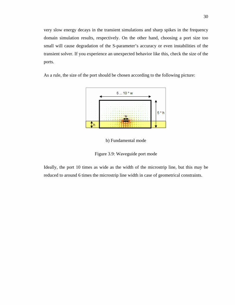
As a rule, the size of the port should be chosen according to the following picture:

b) Fundamental mode

Figure 3.9: Waveguide port mode

Ideally, the port 10 times as wide as the width of the microstrip line, but this may be

reduced to around 6 times the microstrip line width in case of geometrical constraints.

31

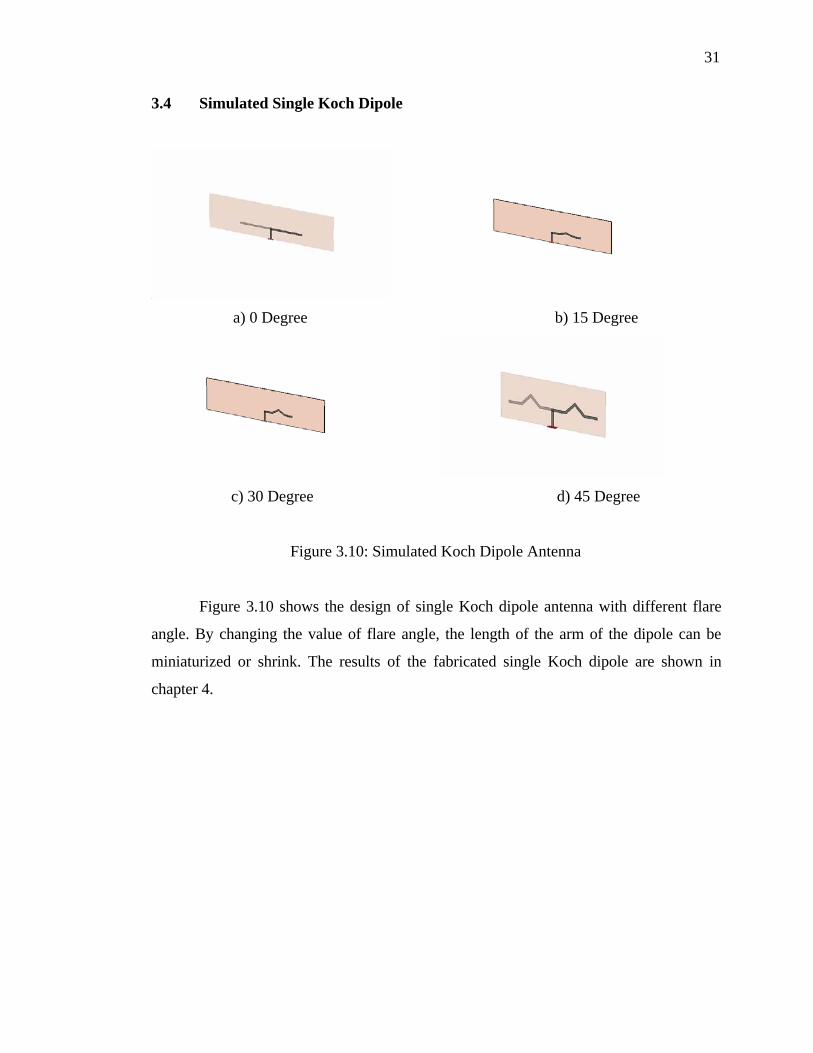
3.4 Simulated Single Koch Dipole

a) 0 Degree b) 15 Degree

c) 30 Degree d) 45 Degree

Figure 3.10: Simulated Koch Dipole Antenna

Figure 3.10 shows the design of single Koch dipole antenna with different flare

angle. By changing the value of flare angle, the length of the arm of the dipole can be

miniaturized or shrink. The results of the fabricated single Koch dipole are shown in

chapter 4.

32

Figure 3.11: Dipole Array Antenna

Figure 3.12: Fractal Koch Dipole Array

33

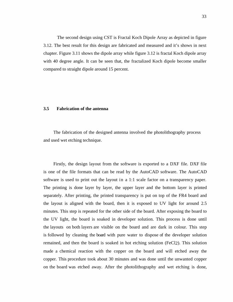
The second design using CST is Fractal Koch Dipole Array as depicted in figure

3.12. The best result for this design are fabricated and measured and it’s shows in next

chapter. Figure 3.11 shows the dipole array while figure 3.12 is fractal Koch dipole array

with 40 degree angle. It can be seen that, the fractalized Koch dipole become smaller

compared to straight dipole around 15 percent.

3.5 Fabrication of the antenna

The fabrication of the designed antenna involved the photolithography process

and used wet etching technique.

Firstly, the design layout from the software is exported to a DXF file. DXF file

is one of the file formats that can be read by the AutoCAD software. The AutoCAD

software is used to print out the layout in a 1:1 scale factor on a transparency paper.

The printing is done layer by layer, the upper layer and the bottom layer is printed

separately. After printing, the printed transparency is put on top of the FR4 board and

the layout is aligned with the board, then it is exposed to UV light for around 2.5

minutes. This step is repeated for the other side of the board. After exposing the board to

the UV light, the board is soaked in developer solution. This process is done until

the layouts on both layers are visible on the board and are dark in colour. This step

is followed by cleaning the board with pure water to dispose of the developer solution

remained, and then the board is soaked in hot etching solution (FeCl2). This solution

made a chemical reaction with the copper on the board and will etched away the

copper. This procedure took about 30 minutes and was done until the unwanted copper

on the board was etched away. After the photolithography and wet etching is done,

34

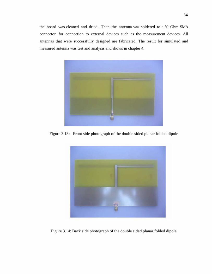
the board was cleaned and dried. Then the antenna was soldered to a 50 Ohm SMA

connector for connection to external devices such as the measurement devices. All

antennas that were successfully designed are fabricated. The result for simulated and

measured antenna was test and analysis and shows in chapter 4.

Figure 3.13: Front side photograph of the double sided planar folded dipole

Figure 3.14: Back side photograph of the double sided planar folded dipole

35

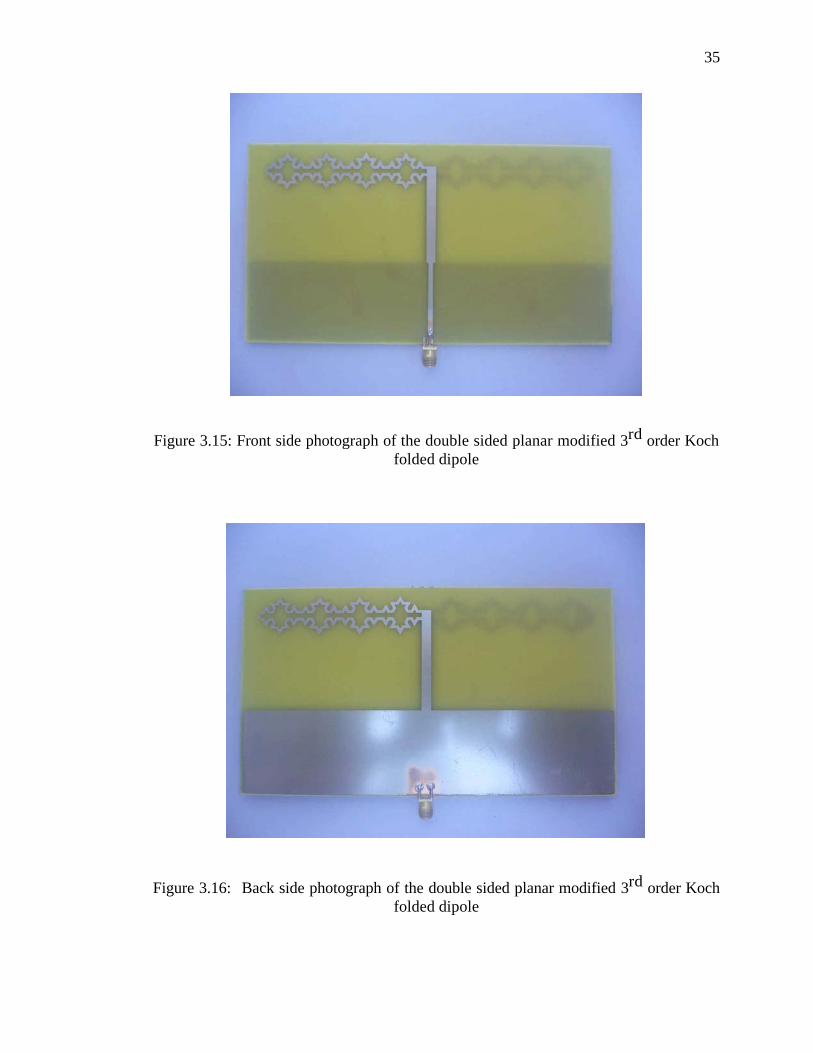
Figure 3.15: Front side photograph of the double sided planar modified 3rd order Koch folded dipole

Figure 3.16: Back side photograph of the double sided planar modified 3rd order Koch

folded dipole

36

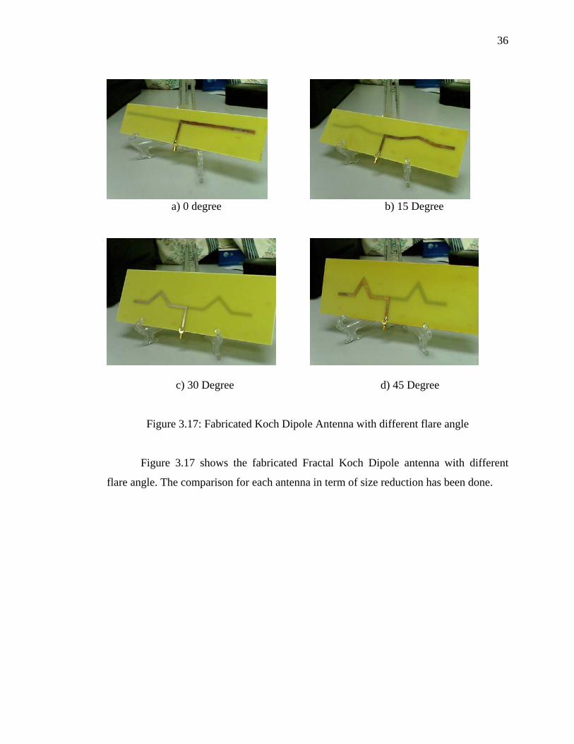
a) 0 degree b) 15 Degree

c) 30 Degree d) 45 Degree

Figure 3.17: Fabricated Koch Dipole Antenna with different flare angle

Figure 3.17 shows the fabricated Fractal Koch Dipole antenna with different

flare angle. The comparison for each antenna in term of size reduction has been done.

37

Figure 3.18: Fabricated Fractal Koch Dipole Array

3.6 Measurements of the Antenna

3.6.1 Input Return Loss Measurement

After fabricating the antenna, testing is done to determine the performance of the

antenna. The property of the antenna that is measured is the input return loss. The return

loss is measured using the Marconi Instruments Microwave Test Set 6204 and Vector

Impedance Analyzer Via Echo V2.5.

After connecting the antenna to this device, the first step in using the Marconi

Instrument is to set the frequency range that will be analyzed. For this antenna, the

frequency range is set to 400 to 900MHz. The next step is to do the calibration.

Calibration is done to ensure the precision of the instrument for any spectrum. After

38

that, measurement is done and the device will sweep the frequency band and plot

the return loss of the antenna and display it on the screen.

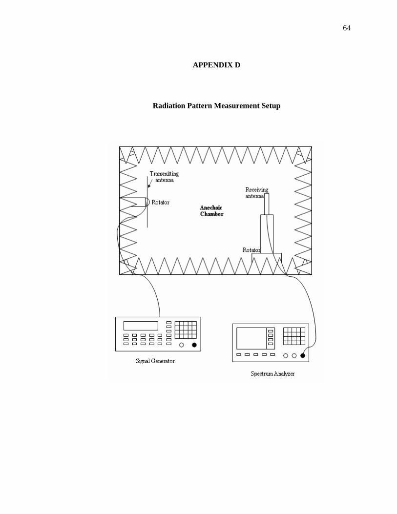
3.6.2 Radiation Pattern Measurement

There is one more property of the antenna that can be measured which is the

radiation pattern. The measurement of radiation pattern requires a signal

generator, transmitting antenna, a rotating machine and a spectrum generator. The

measurement is done in an anechoic chamber which is a special chamber for measuring

signal power of antennas. The antenna under test is attached on the rotating machine.

The antenna designed (antenna under test) will act as a receiving antenna. The

transmitting antenna used is a standard indoor TV dipole antenna with retractable

radials in both directions that makes 180° angle between each other. This dipole

antenna can be stretched and shortened to suit the length of the operating frequency.

Both the receiving and transmitting antenna will be placed aligned to each other in the

chamber.

The measurements are done 6 times, three for the folded straight dipole antenna

and three for the folded Koch antenna. First, the co-polarization in the E plane is

measured. Both the receiving and transmitting antennas are placed in vertical positions.

Then the receiving antenna is rotated 360° while the measured data is collected. The

next step is to measure the cross-polarization in the E plane. The receiving antenna is

placed in a horizontal position. Then the receiving antenna is rotated 360° while

the measured data is collected. The last step is to measure the co-polarization in the H

39

plane. Both the receiving and transmitting antennas are placed in horizontal positions.

Then the receiving antenna is rotated 360° while the measured data is collected.

3.7 Summary

This chapter discusses the design of different kinds of planar dipole antennas

structure. The design includes the standard straight line dipole, the meandered line

dipole antenna, the 3rd order Koch curve dipole, the folded dipole, the folded Koch

curve dipole and fractal Koch dipole array. The design process involves the use of three

antenna design software. One is the AWR Microwave Office, Agilent ADS and

Computer Simulation Technology CST. After designing the layout of the antenna,

simulation is done for each antenna. Simulation is done for the return loss and the 3D

radiation pattern of the antenna. This fabrication process is done using the

photolithography and wet etching technique. After fabrication is finished, the

measurement process is done using the available test equipments in the lab. The results

of the measurement are presented in chapter 4.

CHAPTER 4

RESULTS AND DISCUSSION

4.0 Introduction

The measurement results for passive antenna designed in this project can

first be simulated using the Agilent ADS software and Computer Simulation

Technology CST. This software uses the Method of Moments (MoM) to calculate

and predict the properties of the designed antenna. The simulation is done to get

the predicted values of the input return loss and the radiation pattern of the passive

antennas. The simulation results are based on the antenna designs in Chapter 3.

4.1 Antenna Simulation Results

4.1.1 Standard straight line dipole

Figure 4.1 shows the return loss of the antenna. Here it can be seen that

it has a resonant frequency at about 575 MHz with the return loss value of

41

about -13 dB. The bandwidth is calculated from the lower frequency values

which intercept the -10 dB value of the return loss, until the upper frequency

value which intercept the -10 dB value of the return loss. Calculation from

equation (2) in chapter 2 gives us the bandwidth of 0.7%.

Figure 4.1: Simulated return loss of the standard straight line dipole

Figure 4.2 shows the return loss of the antenna. Here it can be seen that it

has a resonant frequency at about 575 MHz with the return loss of about -24 dB.

The resonant frequency is made the same as the straight line dipole in section

4.2.1. Calculation from equation (2) in chapter 2 gives us the bandwidth of the

meandered line dipole designed about 0.7 %. The meander line dipole shows a

miniaturization characteristic which is shown by the shorter length of the dipole

arms compared to the straight line dipole. With a dimension height of only 7 mm,

the meander managed to decrease the length of the dipole from 177 mm to 143

mm.

42

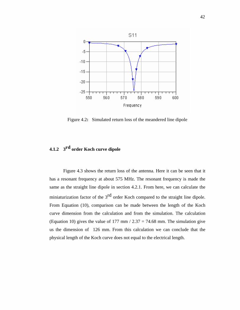
Figure 4.2: Simulated return loss of the meandered line dipole

4.1.2 3rd order Koch curve dipole

Figure 4.3 shows the return loss of the antenna. Here it can be seen that it

has a resonant frequency at about 575 MHz. The resonant frequency is made the

same as the straight line dipole in section 4.2.1. From here, we can calculate the

miniaturization factor of the 3rd order Koch compared to the straight line dipole.

From Equation (10), comparison can be made between the length of the Koch

curve dimension from the calculation and from the simulation. The calculation

(Equation 10) gives the value of 177 mm / 2.37 = 74.68 mm. The simulation give

us the dimension of 126 mm. From this calculation we can conclude that the

physical length of the Koch curve does not equal to the electrical length.

43

Figure 4.3: Simulated return loss of the 3rd order Koch curve dipole

Figure 4.4: Simulated return loss for single Koch dipole antenna with

different angle.

44

The simulated return loss for single Koch dipole antenna as depicted in

figure 4.4 shows that for every increment of the angle, the return loss has a little

bit shifted to the upper frequencies. It’s may be due to the shrinking of the length

of the dipole.

a) Radiation 0 Degree b) Radiation 15 Degree

c) Radiation 30 Degree d) Radiation 45 Degree

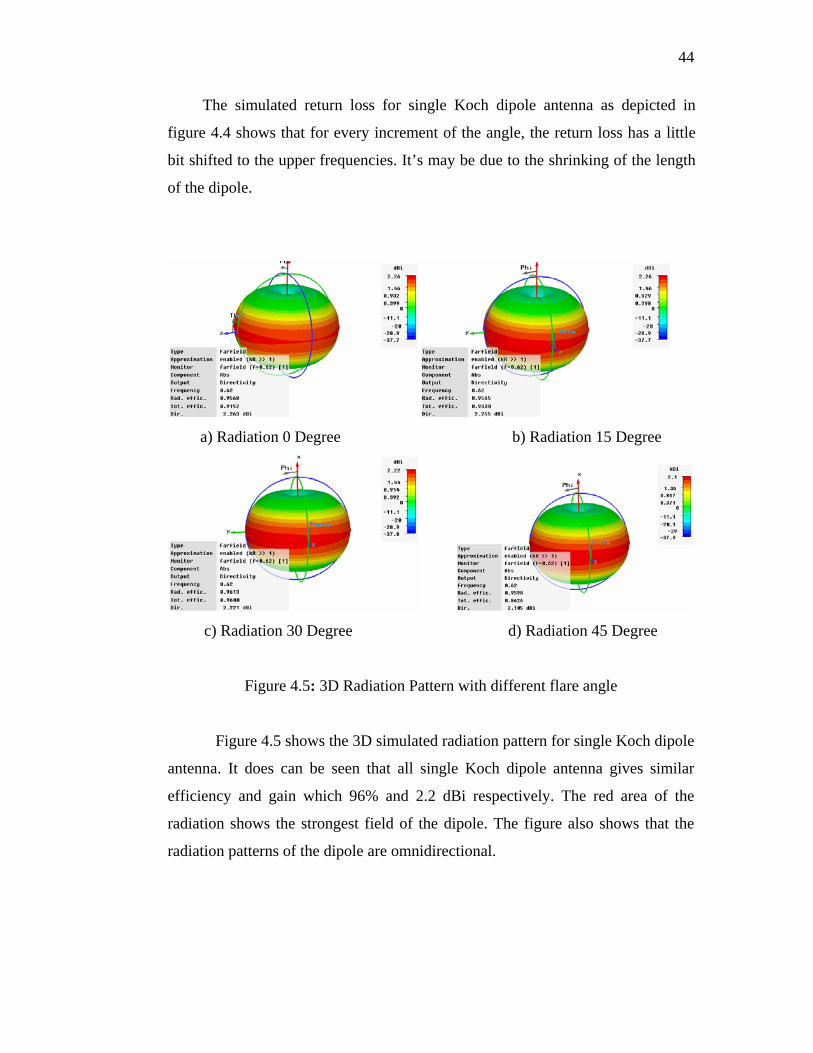
Figure 4.5: 3D Radiation Pattern with different flare angle

Figure 4.5 shows the 3D simulated radiation pattern for single Koch dipole

antenna. It does can be seen that all single Koch dipole antenna gives similar

efficiency and gain which 96% and 2.2 dBi respectively. The red area of the

radiation shows the strongest field of the dipole. The figure also shows that the

radiation patterns of the dipole are omnidirectional.

45

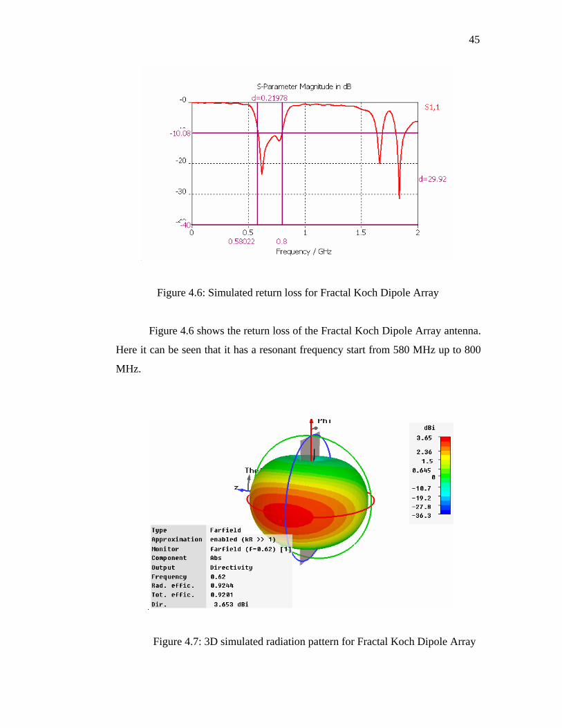
Figure 4.6: Simulated return loss for Fractal Koch Dipole Array

Figure 4.6 shows the return loss of the Fractal Koch Dipole Array antenna.

Here it can be seen that it has a resonant frequency start from 580 MHz up to 800

MHz.

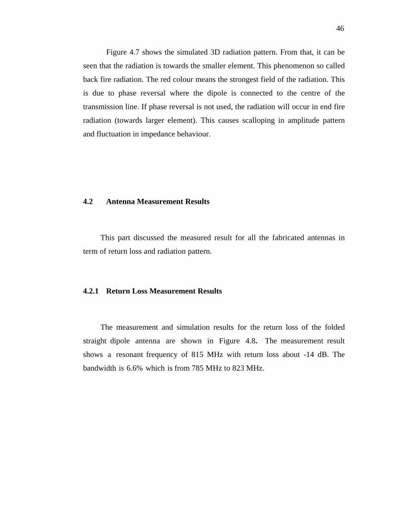
Figure 4.7: 3D simulated radiation pattern for Fractal Koch Dipole Array

46

Figure 4.7 shows the simulated 3D radiation pattern. From that, it can be

seen that the radiation is towards the smaller element. This phenomenon so called

back fire radiation. The red colour means the strongest field of the radiation. This

is due to phase reversal where the dipole is connected to the centre of the

transmission line. If phase reversal is not used, the radiation will occur in end fire

radiation (towards larger element). This causes scalloping in amplitude pattern

and fluctuation in impedance behaviour.

4.2 Antenna Measurement Results

This part discussed the measured result for all the fabricated antennas in

term of return loss and radiation pattern.

4.2.1 Return Loss Measurement Results

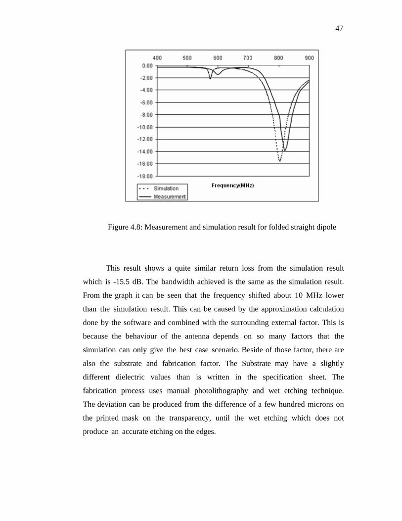
The measurement and simulation results for the return loss of the folded

straight dipole antenna are shown in Figure 4.8. The measurement result

shows a resonant frequency of 815 MHz with return loss about -14 dB. The

bandwidth is 6.6% which is from 785 MHz to 823 MHz.

47

Figure 4.8: Measurement and simulation result for folded straight dipole

This result shows a quite similar return loss from the simulation result

which is -15.5 dB. The bandwidth achieved is the same as the simulation result.

From the graph it can be seen that the frequency shifted about 10 MHz lower

than the simulation result. This can be caused by the approximation calculation

done by the software and combined with the surrounding external factor. This is

because the behaviour of the antenna depends on so many factors that the

simulation can only give the best case scenario. Beside of those factor, there are

also the substrate and fabrication factor. The Substrate may have a slightly

different dielectric values than is written in the specification sheet. The

fabrication process uses manual photolithography and wet etching technique.

The deviation can be produced from the difference of a few hundred microns on

the printed mask on the transparency, until the wet etching which does not

produce an accurate etching on the edges.

48

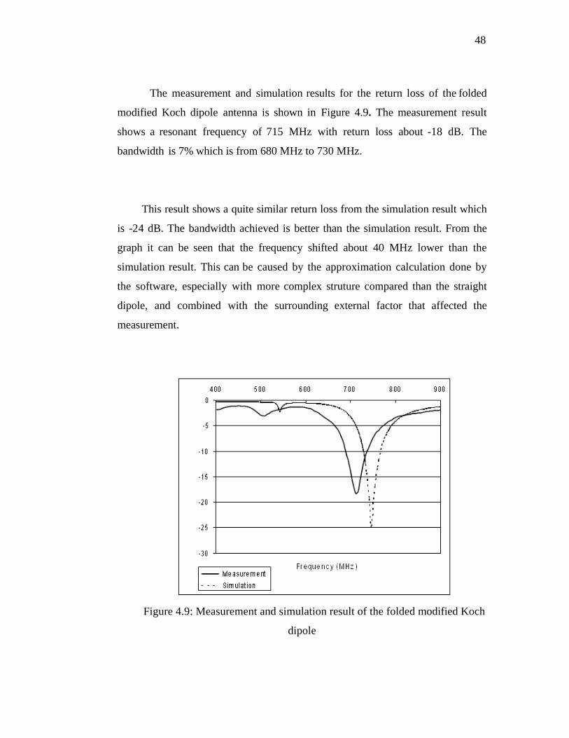
The measurement and simulation results for the return loss of the folded

modified Koch dipole antenna is shown in Figure 4.9. The measurement result

shows a resonant frequency of 715 MHz with return loss about -18 dB. The

bandwidth is 7% which is from 680 MHz to 730 MHz.

This result shows a quite similar return loss from the simulation result which

is -24 dB. The bandwidth achieved is better than the simulation result. From the

graph it can be seen that the frequency shifted about 40 MHz lower than the

simulation result. This can be caused by the approximation calculation done by

the software, especially with more complex struture compared than the straight

dipole, and combined with the surrounding external factor that affected the

measurement.

Figure 4.9: Measurement and simulation result of the folded modified Koch

dipole

49

Simulated and measured return loss

Freq (GHz)

0.0 0.2 0.4 0.6 0.8 1.0 1.2

S11

(dB)

-25

-20

-15

-10

-5

0

MeasuredSimulation

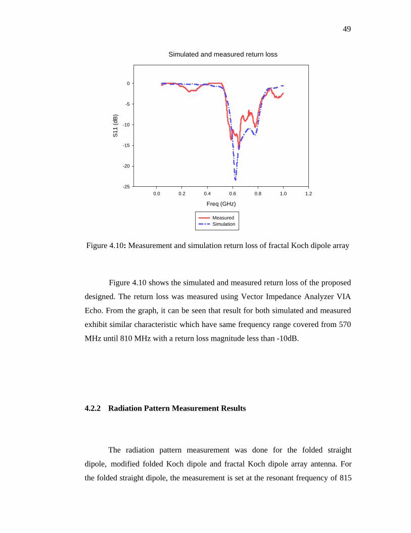
Figure 4.10: Measurement and simulation return loss of fractal Koch dipole array

Figure 4.10 shows the simulated and measured return loss of the proposed

designed. The return loss was measured using Vector Impedance Analyzer VIA

Echo. From the graph, it can be seen that result for both simulated and measured

exhibit similar characteristic which have same frequency range covered from 570

MHz until 810 MHz with a return loss magnitude less than -10dB.

4.2.2 Radiation Pattern Measurement Results

The radiation pattern measurement was done for the folded straight

dipole, modified folded Koch dipole and fractal Koch dipole array antenna. For

the folded straight dipole, the measurement is set at the resonant frequency of 815

50

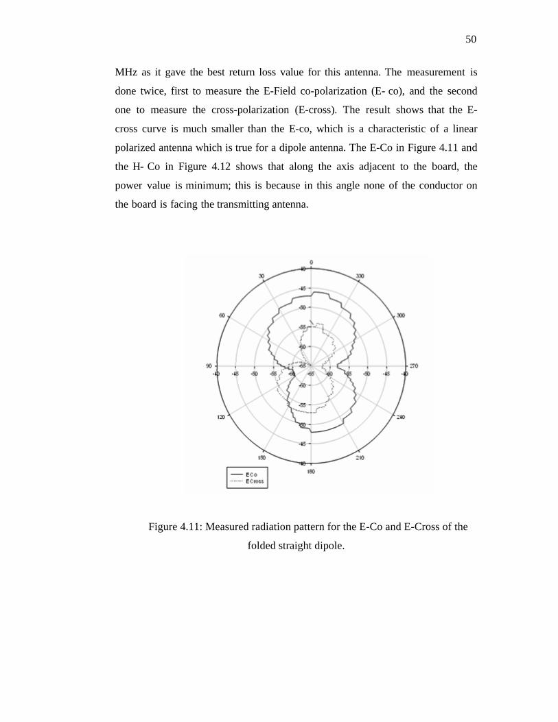
MHz as it gave the best return loss value for this antenna. The measurement is

done twice, first to measure the E-Field co-polarization (E- co), and the second

one to measure the cross-polarization (E-cross). The result shows that the E-

cross curve is much smaller than the E-co, which is a characteristic of a linear

polarized antenna which is true for a dipole antenna. The E-Co in Figure 4.11 and

the H- Co in Figure 4.12 shows that along the axis adjacent to the board, the

power value is minimum; this is because in this angle none of the conductor on

the board is facing the transmitting antenna.

Figure 4.11: Measured radiation pattern for the E-Co and E-Cross of the

folded straight dipole.

51

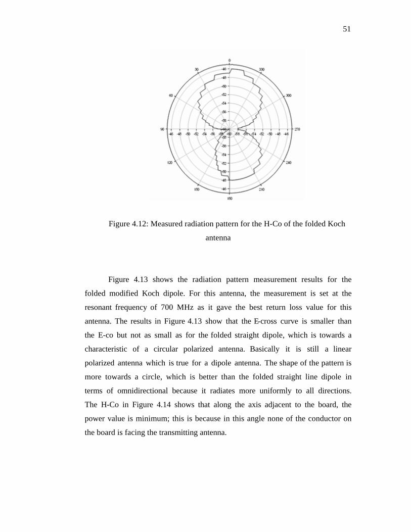
Figure 4.12: Measured radiation pattern for the H-Co of the folded Koch

antenna

Figure 4.13 shows the radiation pattern measurement results for the

folded modified Koch dipole. For this antenna, the measurement is set at the

resonant frequency of 700 MHz as it gave the best return loss value for this

antenna. The results in Figure 4.13 show that the E-cross curve is smaller than

the E-co but not as small as for the folded straight dipole, which is towards a

characteristic of a circular polarized antenna. Basically it is still a linear

polarized antenna which is true for a dipole antenna. The shape of the pattern is

more towards a circle, which is better than the folded straight line dipole in

terms of omnidirectional because it radiates more uniformly to all directions.

The H-Co in Figure 4.14 shows that along the axis adjacent to the board, the

power value is minimum; this is because in this angle none of the conductor on

the board is facing the transmitting antenna.

52

Figure 4.13: Measurement result for E-Co and E Cross of the folded Koch dipole

Figure 4.14: Measurement results for the H-Co radiation pattern of the folded

Koch dipole

53

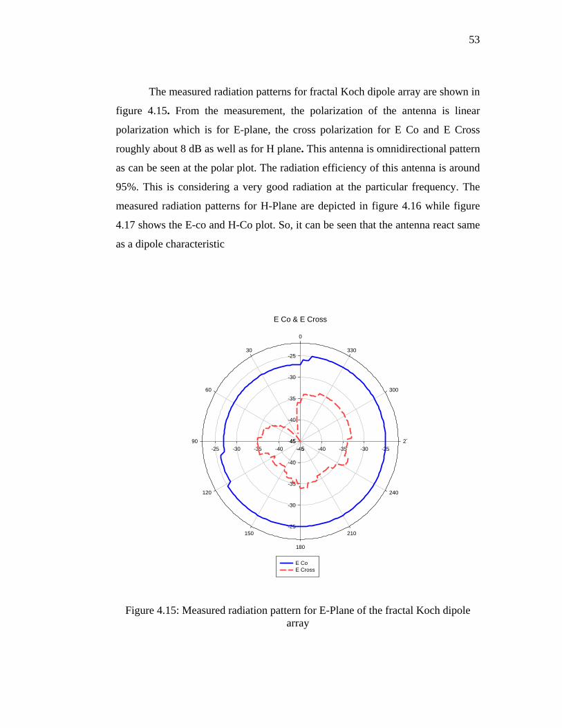
The measured radiation patterns for fractal Koch dipole array are shown in

figure 4.15. From the measurement, the polarization of the antenna is linear

polarization which is for E-plane, the cross polarization for E Co and E Cross

roughly about 8 dB as well as for H plane. This antenna is omnidirectional pattern

as can be seen at the polar plot. The radiation efficiency of this antenna is around

95%. This is considering a very good radiation at the particular frequency. The

measured radiation patterns for H-Plane are depicted in figure 4.16 while figure

4.17 shows the E-co and H-Co plot. So, it can be seen that the antenna react same

as a dipole characteristic

E Co & E Cross

-45 -40 -35 -30 -25-45

-40

-35

-30

-25

-45-40-35-30-25-45

-40

-35

-30

-25

0

30

60

90

120

150

180

210

240

27

300

330

E Co E Cross

Figure 4.15: Measured radiation pattern for E-Plane of the fractal Koch dipole array

54

H Co & H Cross

-55 -50 -45 -40 -35 -30 -25-55

-50

-45

-40

-35

-30

-25

-55-50-45-40-35-30-25-55

-50

-45

-40

-35

-30

-25

0

30

60

90

120

150

180

210

240

27

300

330

H Co H Cross

Figure 4.16: Measured radiation pattern for H- Plane of the fractal Koch dipole array

Radiation Pattern E & H Plane

-55 -50 -45 -40 -35 -30 -25-55

-50

-45

-40

-35

-30

-25

-55-50-45-40-35-30-25-55

-50

-45

-40

-35

-30

-25

0

30

60

90

120

150

180

210

240

27

300

330

E Co H Co

Figure 4.17: Measured Co & Cross Polar of the fractal Koch dipole array

55

4.3 Summary

This chapter has presented the simulation results of all designed antenna

and the measurement results of the fabricated antennas that serve the purpose

of the project. Both simulation and measurement for the return loss shows similar

results with a slightly shift of resonant frequency. The bandwidth of the

fabricated antenna is 7% which is quite small compared to the terrestrial TV

frequency band. Although the radiation pattern did not exactly resemble the

theoretical pattern, but it still shows a characteristic of a dipole antenna which

is omnidirectional.

CHAPTER 5

CONCLUSION AND FUTURE WORK

5.0 Conclusion

The design of the planar dipole fractal antenna for the UHF band has been

presented. The work includes designing, simulating, fabricating, and measuring

the return loss and radiation pattern of the proposed antenna has been done. The

designing process is based on different designs that have been proposed in

published journals. The design and simulation is done using simulation software

such as Applied Wave Research AWR, Agilent ADS 2004A and Computer

Simulation Technology CST. Simulation is done to help the user know the

predicted properties of the antenna before fabricating the antenna since only little

calculations from literatures are provided for this kind of antenna. The fabrication

involves photolithography and wet etching which gives adequate result for this

type of antenna.

The simulation gives a bandwidth value of 5 % and the measurement gives a

bandwidth value of 7 % which is quite small compared to the terrestrial TV

frequency band. The simulation of the radiation pattern gives an omnidirectional

pattern while the measurement does not quite give an omnidirectional pattern (the

power is not the same in all direction) but it still radiates to all directions.

57

The folded dipole configuration can be used to increase bandwidth of a

standard dipole.

The Koch fractal can be used to miniaturize the length of a standard straight line dipole.

The Koch fractal can be used to miniaturize the length of a standard straight line dipole.

The fractal Koch dipole array can used to reduce the length of the straight

dipole and also to increase the bandwidth.

5.1 Proposed Future Work

Further works should be carried out in order to improve the bandwidth

of the antenna:

1. Different configuration can be used such as the log periodic to get

multiresonant frequencies to achieve wider bandwidth. But these methods

will result a quite large dimension antenna.

2. Different kinds of dimension of the dipole arms can be experimented to find

the optimum values for wider bandwidth.

3. Using a different kind of planar structure such as the single side planar with

surrounding ground plane could give a better bandwidth.

58

REFERENCES

1. Puente, C., Romeu, J., Pous, R., Ramis, J., and Hijazo, A. (1998) . Small But

Long Koch Fractal Monopole. IEEE Electronic Letters, 34(1): 9-10.

2. Breden, R., and Langley, R.J. (1999). Printed Fractal Antennas. IEEE National

Conference on Antennas and Propagation. pp. 1-4.

3. Stutzmann,Warren L. and Thiele, Garry A..Antenna Theory and Design . 2nd

Ed. New York: John Wiley and Sons. 1998.

4. Johnson, H. and Graham, M. High-Speed Digital Design. New Jersey: Prentice-

Hall.1993.

5. Vinoy, K. J., Abraham, J.K., and Varadan, V.K. (2003). On the Relationship

Between Fractal Dimension and the Performance of Multi-Resonant Dip ole

Antennas Using Koch Curves. IEEE Transactions on Antennas and

Propagation. 51(9).

6. Chen, H.M., Chen, J.M., Chengand, P.S., and Lin, Y.F. (2004) . Feed for dual-

band printed dipole antenna. Electronics Letters. 40(21).

7. Puente, C., Romeu, J., and Cardama, A. (2000). The Koch Monopo le: A

Small Fractal Antenna. IEEE Transactions On Antennas And Propagation. 48(11).

59

8. Wemer, D. , Haupt, R.L., and Wemer, P.L. ( 1999). Fractal antenna engineering:

The theory and design of fractal antenna arrays. IEEE Antennas and

Propagation Magazine. 41(5):37-59.

9. Best, S.R. (2002). On the resonant properties of the Koch fractal and other

wire monopole antennas. IEEE Antennas and Wireless Propagation Letters. 1(1).

11. Best, S.R. (2003). A discussion on the significance of geometry in determining

the resonant behavior of fractal and other non-Euclidean wire antennas. IEEE

Antennas and Propagation Magazine, 45(3):9-28.

12. Vinoy, K. J., Abraham, J.K., and Varadan, V.K. (2003). Fractal dimension

and frequency response of fractal shaped antennas. IEEE Antennas and

Propagation Society International Symposium . 22-27 June. Volume 4 ,222 – 225 .

13. Werner, D.H., and Ganguly, S. (2003). An overview of fractal antenna

engineering research. IEEE Antennas and Propagation Magazine. 45(1):38 - 57.

14. Eason, S.D., Libonati, R., Culver, J.W., Werner, D.H., Werner, P.L.,

and Mummareddy, S. (2001). UHF fractal antennas. IEEE Antennas and

Propagation Society International Symposium . 8-13 July. Volume 3, 636 – 639.

15. Tang, P. (2001). Scaling property of the Koch fractal dipole. IEEE Antennas

and Propagation Society International Symposium . 8-13 July. Volume 3, 150 –

153.

16. Breden, R., and Langley, R.J. (1999). Printed fractal antennas. IEEE

National Conference on Antennas and Propagation. March-1 April. Page(s):1– 4,

60

17. An Hongming, Nauwelaers, B.K.J.C., and Van de Capelle, A.R. (1994).

Broadband active microstrip antenna design with the simplified real frequency

technique. IEEE Transactions on Antennas and Propagation. 42(12):1612 - 1619.

18. Suh, Young-Ho, and Chang, Kai. (2000). Low cost microstrip- fed dual

frequency printed dipole antenna for wireless communications. IEEE Electronics

Letters, 36(14):1177 - 1179.

19. Cohen, N. (1996). Fractal and shaped dipoles. Commun. Quart .,25–36.

20. Karnfelt, C., Hallbjorner, P., Zirath, H., and Alping, A. (2006). High gain

active microstrip antenna for 60-GHz WLAN/WPAN applications. IEEE

Transactions on Microwave Theory and Techniques. 54 (6):2593 – 2603.

21. Li, J. (1993). Direction and polarization estimation using arrays with small loops

and short dipoles. IEEE Transactions on Antennas and Propagation. 41(3) :379 -

387.

22. Sarabandi,K. and Azadegan, R. (2003). Design of an efficient miniaturized

UHF planar antenna. IEEE Transactions on Antennas and Propagation. 51(6)

:1270 -1276.

23. Hsiao,Fu-Ren and Wong, Kin-Lu (2004). Omnidirectional planar folded dipole

antenna. IEEE Transactions on Antennas and Propagation. 52(7):1898 – 1902.

61

APPENDIX A

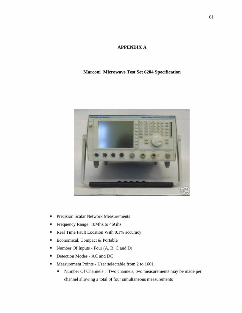
Marconi Microwave Test Set 6204 Specification

Precision Scalar Network Measurements

Frequency Range: 10Mhz to 46Ghz

Real Time Fault Location With 0.1% accuracy

Economical, Compact & Portable

Number Of Inputs - Four (A, B, C and D)

Detection Modes - AC and DC

Measurement Points - User selectable from 2 to 1601

Number Of Channels : Two channels, two measurements may be made per

channel allowing a total of four simultaneous measurements

62

APPENDIX B

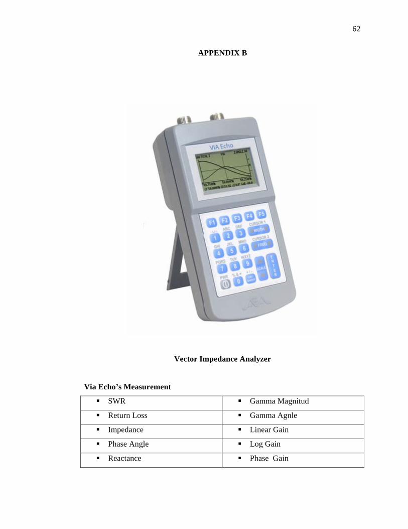
Vector Impedance Analyzer

Via Echo’s Measurement

SWR Gamma Magnitud

Return Loss Gamma Agnle

Impedance Linear Gain

Phase Angle Log Gain

Reactance Phase Gain

63

APPENDIX C

64

APPENDIX D

Radiation Pattern Measurement Setup

1

UTM/RMC/F/0014 (1998)

UNIVERSITI TEKNOLOGI MALAYSIA Research Management Centre

PRELIMINARY IP SCREENING & TECHNOLOGY ASSESSMENT FORM

(To be completed by Project Leader submission of Final Report to RMC or whenever IP protection arrangement is required) 1. PROJECT TITLE IDENTIFICATION :

DESIGN AND DEVELOPMENT OF FRACTAL ANTENNA FOR UHF BAND APPLICATION nteractive Contrasting Learniations Study Skills and Academic Achievements

Vote No: 78034

2. PROJECT LEADER :

Name : PROF. MADYA DR. M0HAMAD KAMAL A. RAHIM

Address : JABATAN KEJURUTERAAN RADIO, FAKULTI KEJURUTERAAN ELEKTRIK,

UNIVERSITI TEKNOLOGI MALAYSIA, 81310 SKUDAI, JOHOR

Tel : 07 5536088 Fax : - 07-5566272 e-mail : mkamal@fke.utm.my

3. DIRECT OUTPUT OF PROJECT (Please tick where applicable)

4. INTELLECTUAL PROPERTY (Please tick where applicable) Not patentable Technology protected by patents

Patent search required Patent pending

Patent search completed and clean Monograph available

Invention remains confidential Inventor technology champion

No publications pending Inventor team player

No prior claims to the technology Industrial partner identified

Scientific Research Applied Research Product/Process Development Algorithm Method/Technique Product / Component Structure Demonstration / Process Prototype Data Software

Other, please specify Other, please specify Other, please specify ___________________ __________________ ___________________________ ___________________ __________________ ___________________________ ___________________ __________________ ___________________________

79018

Lampiran 13

2

UTM/RMC/F/0014 (1998)

5. LIST OF EQUIPMENT BOUGHT USING THIS VOT

• Computer Simulation Technology (CST) and AWR Microwave Office (Rental)

• Handheld Spectrum Analyzer (UP TO 3 GHz)

• Handheld Vector Impedance Analyzer (Via Eco)

___________________________________________________________________________

___________________________________________________________________________

6. STATEMENT OF ACCOUNT

a) APPROVED FUNDING RM : 176,796.00

b) TOTAL SPENDING RM : 176,681.49

c) BALANCE RM : 114.51

7. TECHNICAL DESCRIPTION AND PERSPECTIVE

Please tick an executive summary of the new technology product, process, etc., describing how it works. Include brief analysis that compares it with competitive technology and signals the one that it may replace. Identify potential technology user group and the strategic means for exploitation. a) Technology Description

This  project  begins  with  understanding  the  concept  of  the  planar  structure  antenna technologies  and    Fractal  antenna  behavior  .  This  includes  the  properties  such  as radiation  pattern,  input  impedance,  bandwidth,  beamwidth  and  operating  frequency. The design and  simulation has been caried out using  comercial  software  ie: Computer Simulation  Technology  CST  and  Applied  Wave  Research  AWR.  The  practical implementation  has  been  carried  out  after  the  simulation  process  completed.  The comparisons  between  simulation  and  experimental have  been made  in  term  of  return loss,  bandwidth  and  radiation  pattern.  It  shows  that  the  fractal UHF  antenna  can  be reduced  the  size  of  planar  dipole  antenna  by  20  percent  from  the  original  planar structure. 

b) Market Potential

Suitable for wireless industries that operating in the UHF band application.

____________________________________________________________________________

3

c) Commercialisation Strategies

This product suitable for UHF band application. So, for the cormerciallization need some extra

work and funding for final packaging of the product.

____________________________________________________________________________

____________________________________________________________________________

____________________________________________________________________________ 8. RESEARCH PERFORMANCE EVALUATION

a) FACULTY RESEARCH COORDINATOR Research Status ( ) ( ) ( ) ( ) ( ) ( ) Spending ( ) ( ) ( ) ( ) ( ) ( ) Overall Status ( ) ( ) ( ) ( ) ( ) ( ) Excellent Very Good Good Satisfactory Fair Weak

Comment/Recommendations : _____________________________________________________________________________

_____________________________________________________________________________

_____________________________________________________________________________

_____________________________________________________________________________

_____________________________________________________________________________

_____________________________________________________________________________

………………………………………… Name : ………………………………………

Signature and stamp of Date : ……………………………………… JKPP Chairman

UTM/RMC/F/0014 (1998)

4

RE

b) RMC EVALUATION

Research Status ( ) ( ) ( ) ( ) ( ) ( ) Spending ( ) ( ) ( ) ( ) ( ) ( ) Overall Status ( ) ( ) ( ) ( ) ( ) ( ) Excellent Very Good Good Satisfactory Fair Weak

Comments :- _____________________________________________________________________________

_____________________________________________________________________________

_____________________________________________________________________________

_____________________________________________________________________________

_____________________________________________________________________________

_____________________________________________________________________________ Recommendations :

Needs further research

Patent application recommended

Market without patent

No tangible product. Report to be filed as reference

……………………………………….. Name : ……………………………………………

Signature and Stamp of Dean / Date : …………………………………………… Deputy Dean Research Management Centre

UTM/RMC/F/0014 (1998)

End of Project Report 1 January 2006 ScienceFund

End of Project Report For ScienceFund

A. Description of the Project

1. Project number: 79018

2. Project title: DESIGN AND DEVELOPMENT OF FRACTAL ANTENNA FOR UHF BAND APPLICATION

3. Project leader: Assoc. Prof Dr Mohamad Kamal A Rahim

4. Project Team:

(Please provide an assessment of how the project team performed and highlight any significant departures from plan in either structure or actual man-days utilised)

Assoc. Prof. Dr. Mohammad Kamal A. Rahim Mr Nazri A. Karim Mr. Thelaha Masri Mr Huda A. Majid Mr Osman Ayop

5. Industrial Partnership: (Please describe the nature of collaborations with relevant industry) At this moment, no collaborations with relevant industries involve.

6. National/International Collaboration (please identify research organisations and describe the nature of collaboration) No research organisation involve.

7. Project Duration: ____21____months

8. Budget Approved: RM 176,769.00

B. Objectives of the project

1. Socio-economic Objectives (SEO)

Which socio-economic objectives are addressed by the project? (Please identify the Research Priority Area , SEO Category and SEO Group under which the project falls. Refer to the Malaysian R&D Classification System, 4th Edition. Research Priority Area SEO Category: Information Communication and Technology (ICT) SEO Group : Communication Sevices 2. Fields of Research (FOR)

Which are the two main FOR Categories, FOR Groups, and FOR Areas of your project? (Please refer to the Malaysian R&D Classification System, 4th Edition)

a. Primary field of research

FOR Category: Information Communication and Technology (ICT) FOR Group : Communication FOR Area: Antenna Technology b. Secondary Field of research

FOR Category: Information Communication and Technology (ICT) FOR Group : Communication FOR Area: Wireless Communication and Technologies

End of Project Report 2 January 2006 ScienceFund

C. Objectives achievement

• Original project objectives (Please state the specific project objectives as described in Section II of the Application Form)

1. To design and develop a new structure of fractal antenna design for multiband operating frequency. 2. To develop a prototype fractal antenna for Ultra High Frequency Wireless RAN technology

• Objectives Achieved (Please state the extent to which the project objectives were achieved) New structure of fractal antenna has been succesfully designed and fabricated operating at UHF

band application. The protoyped of this antenna has been tested and verify with the simulation using CST software.

• Objectives not achieved (Please identify the objectives that were not achieved and give reasons) D. Technology Transfer/Commercialisation Approach, if any. (Please describe the approach

planned to transfer/commercialise the results of the project)

A new structure of Fractal antenna has been successfully designed and fabricated. For a commerciallisation approach, it’s need some extra work in a market planning and need some funding for that task.

E. Assessment of Research Approach (Please highlight the main steps actually performed and indicate any major departure from the planned approach or any major difficulty encountered)

According to the project schedule. F. Assessment of the Project Schedule (Please make any relevant comment regarding the actual

duration of the project and highlight any significant variation from plan)

Project folllow as schedule

G. Assessment of Project Costs (Please comment on the appropriateness of the original budget and highlight any major departure from the planned budget)

According to the buddget given.

H. Additional Project Funding Obtained (In case of involvement of other funding sources, please indicate the source and total funding provided)

No additional funding.

I. Benefits of the Project (Please identify the actual benefits arising from the project as defined in Section III of the Application Form. For examples of outputs, organisational outcomes and sectoral/national impacts, please refer to Section III of the Guidelines for the Application of R&D Funding under ScienceFund)

Prototype of the antenna operating at UHF band using planar structure.

1. Direct Outputs of the Project (please describe as specifically as possible the outputs achieved and provide an assessment of their significant to users)

i . Technical contribution of the project

a. What was the achieved direct output of the project: For basic oriented research projects ?

Algorithm Structure Data Other, please specify:

End of Project Report 3 January 2006 ScienceFund

For applied research (technology development) projects: Method/technique Demonstrator/prototype Antenna Prototype operating at UHF band.

Product/component Process Software Other, please specify: b. How would you characterise the quality of this output?

Significant breakthrough Major improvement Minor improvement ii. Contribution of the project to knowledge

a. How has the output of the project been documented?

Detailed project report Product/process specification documents Other, please specify: Papers publication b. Did the project create an intellectual property stock?

Patent obtained Patent pending Patent application will be filed Copyright c. What publications are available?

Articles (s) in scientific publications How many: Paper(s) delivered at conferences/seminars How many: 2 papers Book Other, please specify:

End of Project Report 4 January 2006 ScienceFund

d. How significant are citations of the results?

Citations in national publications How many: Citations in international publications How many: None yet Not known

2. Organisational Outcomes of the Project (Please describe as specifically as possible the organisational benefits arising from the project and provide an assessment of their significance)

i. Contribution of the project to expertise development

a. How did the project contribute to expertise?

PhD degrees How many: MSc degrees How many: 2 Research staff with new specialty How many: Other, please specify: b. How significant is this expertise?

One of the key areas of priority for Malaysia (ICT Research Area)

An important area, but not a priority one ii. Economic contribution of the project?

a. How has the economic contribution of the project materialised?

Sales of manufactured product/equipment Royalties from licensing Cost savings Time savings Other, please specify: b. How important is this economic contribution?

High economic contribution Value: RM Medium economic contribution Value: RM - Low economic contribution Value: RM

End of Project Report 5 January 2006 ScienceFund

c. When has this economic contribution materialised?

Already materialised Within months of project completion Within three years of project completion Expected in three years or more Unknown iii. Infrastructural contribution of the project

a. What infrastructural contribution has the project had?

New equipment (Spectrum & Eco analyzer)

Value: RM 59 000.00

New/improved facility Investment: RM New information networks Other, please specify: b. How significant is this infrastructural contribution for the organisation?

Not significant/does not leverage other projects Moderately significant Very significant/significantly leverages other projects iv. Contribution of the project to the organisation’s reputation

a. How has the project contributed to increasing the reputation of the

organisation

Recognition as a Center of Excellence National award International award Demand for advisory services Invitations to give speeches on conferences Visits from other organisations Other, please specify:

End of Project Report 6 January 2006 ScienceFund

b. How important is the project’s contribution to the organisation’s reputation?

Not significant Moderately significant Very significant

3. National Impacts of the Project (If known at this point in time, please describe as specifically as possible the potential sectoral/national benefits arising from the project and provide an assessment of their significance)

i. Contribution of the project to organisational linkages

a. Which kinds of linkages did the project create?

Domestic industry linkages International industry linkages Linkages with domestic research institutions, universities Linkages with international research institutions, universities b. What is the nature of the linkages?

Staff exchanges Inter-organisational project team Research contract with a commercial client Informal consultation Other, please specify: ii. Social-economic contribution of the project

a. Who are the direct customer/beneficiaries of the project output?

Customers/beneficiaries: Number: Wireless industries / wireless subscriber To all wireless communication industries using

UHF band.

b. How has/will the socio-economic contribution of the project

materialised?

Improvements in health Improvements in safety Improvements in the environment Improvements in energy consumption/supply

End of Project Report 7 January 2006 ScienceFund

Improvements in international relations Other, please specify: Improvement in wireless engineering knowledgement c. How important is this socio-economic contribution?

High social contribution Medium social contribution Low social contribution d. When has/will this social contribution materialised?

Already materialised Within three years of project completion Expected in three years or more Unknown Date: 12 August 2008

Signature: