Peperiksaan Semester PertamaSidang Akademik 2004/2005

Sila pastikan bahawa kertas peperiksaan ini mengandungi DUA PULUH EMPAT[24] muka surat yang bercetak sebelum anda memulakan peperiksaan ini .

Jawab semua empat soalan .

UNIVERSITI SAINS MALAYSIA

Oktober 2004

MSG 366 - ANALISIS MULTIVARIAT

Masa : 3 jam

(i)

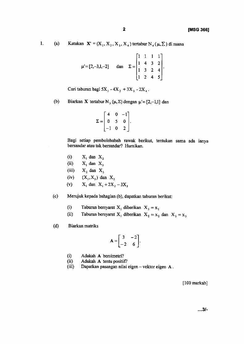
Adakah A bersimetri?(ii)

Adakah A tentu positif?(iii)

Dapatkan pasangan nilai eigen - vektor eigen A.

[100 markah]

2 [MSG 366]

(a) Katakan X' = (X I I X 21 X 31 X4) tertabur N4 (W,E) di mana

1 1 1 1

g'= [2,-3,1,-2] dan1 4

E3 2

=1 3 2 41 2 4 5-

Cari taburan bagi 5X, - 4X -2 + 3X 3 2X 4 .

(b) Biarkan X tertabur N3 (la, E) dengan p.'= [2,-1,1] dan

4 0 -1E= 0 5 0

-1 0 2 -

Bagi setiap pembolehubah rawak berikut, tentukan sama ada ianyabersandar atau tak bersandar? Huraikan .

(i) X, dan X2(ii) X, dan X3(iii) X2 dan X3(iv) (X, , X3) dan X2

(v) X, dan X, + 2X2 - 3X3

(c) Merujuk kepada bahagian (b), dapatkan taburan berikut :

(i) Taburan bersyarat X, diberikan X3 = x3(ii) Taburan bersyarat X, diberikan X2 = x2 dan X3 = x3

(d) Biarkan matriks

2 .

(a)

Pertimbangkan matriks data

3

[MSG 366]

9 1X= 5 3

1 2Terdapat n = 3 cerapan pada p = 2 pembolehubah X, clan XZ . Bentukkangabungan-gabungan linear

c' X = [-1

2][XX

' ( _ -X, + 2X22

b'X=[2 3] f-X'J=2X,+3X22

(i)

Dapatkan min-min sampel, varians clan kovarians bagi b'X clanc'X dari prinsip-prinsip asas . (Petunjuk : kira nilai-nilai yangdicerapi bagi b'X clan c'X, clan kemudian gunakan rumus-rumusmin sampel, varians clan kovarians .)

(ii)

Dapatkan min-min sampel, varians clan kovarians bagi b' X clanc' X

dengan menggunakan

W!,

c'z ,

b'Sb ,

c'Sc , clan

b'Sc ,masing-masing . Bandingkan keputusan-keputusan dalam (i) clan(ii) .

(b)

Cerapan-cerapan pada dua balasan, X, clan X 2 , clikutip bagi tiga rawatan .

(i)

Binakan suatujadual MANOVA satu hala bagi data ini .

(ii)

Nilaikan Lambda Wilks clan ujikan bagi kesan rawatan . Gunakana = 0.01 .

(iii)

Ulangkan ujian dengan menggunakan penghampiran khi-kuasa duadengan pembetulan Bartlett. Bandingkan keputusan-keputusan .

[100 markah]

Vektor-vektor cerapan x' = (x, x 2 ) .

Rawatan 1 : [7 6], [9 5]Rawatan 2 : [3 3], [6 1]Rawatan 3 : [3 2], [1 5]

3.

(a)

(i)

Dengan menggunakan data

I9 6X= 6 10

3 8nilaikan Tz Hotelling untuk menguj i H . : p'= (5, 9) .

(ii)

Nyatakan taburan T Z bagi keadaan dalam (i) di atas .

Nyataandaian-andaian yang telah anda gunakan .

(iii)

Dengan menggunakan (i) dan (ii) di atas, ujikan H o pada parasa =0.01 . Apakah kesimpulan anda?

(b)

Tuliskan nota pendek tentang tajuk-tajuk di bawah:

(i) MANOVA(ii)

Analisis faktor(iii)

Analisis pembezalayan(iv)

Analisis kelompok[100 markah]

4 .

Satu soalselidik dikendalikan atas pelanggan-pelanggan syarikat `Hair, Andersondan Tatham Company' (HATCO), sebuah pembekal industri (industrial supplier) .Sebuah firma penyelidikan pemasaran mengutip data soalselidik HATCO.Pangkalan datanya terdiri daripada 100 cerapan bagi setiap 14 pembolehubah .Tiga jenis maklumat dikutip . Jenis yang pertama ialah persepsi pelangganterhadap HATCO ke atas tujuh atribut yang dicamkan dalam kajian-kajian lepassebagai atribut yang sangat mempengaruhi pilihan pembekal . Responden-responden, iaitu pengurus-pengurus pembelian (purchasing managers) bagi firma-firma yang membeli dari HATCO, menilai HATCO ke atas setiap atribut .Maklumat jenis yang kedua berkenaan dengan keputusan pembelian yangsebenar, sama ada penilaian kepuasan dengan HATCO bagi setiap responden atauperatusan pembelian produk responden dari HATCO. Maklumat jenis yang ketigamengandungi ciri am syarikat pembelian (misalnya, saiz firma, jenis industri) .

Data yang dikutip harus memberi HATCO suatu pemahaman yang baik tentangciri-ciri pelanggannya dan perhubungan antara persepsi pelanggan terhadapHATCO dan tindakan pelanggan terhadap HATCO (pembelian dan kepuasan) .Takrif bagi setiap pembolehubah dan penerangan kodnya diberi dalam bahagian-bahagian yang berikut .

I.

Persepsi Pelauggan

5

[MSG 366]

Setiap pembolehubah disukat atas satu skala graft, yang mana satu garis 10sentimeter dilukis antam tifk dilabel `Lemah' dan ffk dilabel `Cemerlang' .Responden menunjukkan persepsinya dengan membuat satu tanda pada mana-mana garis itu. Tanda disukat dan jarak dari 0 (dalam sentimeter) direkod.Keputusan adalah satu skala dari 0 hingga 10, dibundarkan kepada satu tempatperpuluhan . Tujuh atribut HATCO yang dinilai oleh setiap responden adalahseperti berikut:

X I :

Kelajuan penghantaran (Delivery speed) - amaun masa yang diambiluntuk menghantar produk setelah permintaan disahkan .

X2 :

Paras harga (Price level) - persepsi paras harga yang ditetapkan olehpembekal-pembekal produk .

X3 :

Fleksibiliti harga (Price flexibility) - persepsi kesediaan wakil-wakilHATCO untuk merunding hargapada semua jenis pembelian .

X4 :

Imej pengeluar ( Manufacturer's image) - imej keseluruhan pengeluaratau pembekal .

XS :

Perkhidmatan

keseluruhan

(Overall

service)

-

paras

keseluruhanperkhidmatan yang diperlukan untuk menjaga perhubungan yangmemuaskan antara pembekal dan pembeli.

X6 :

Imej pasukan jualan (Salesforce image) - imej keseluruhan bagi pasukanjualan pengeluar .

X, :

Kualiti produk (Product quality) - persepsi paras kualiti bagi suatu produk(misalnya, prestasi atau hasil) .

II .

Keputusan Pembelian

X8 :

Paras gunaan (Usage level) - berapa banyak jumlah produk dibeli dariHATCO, disukat pada satu skala peratusan 100-titik, berjulat dari 0 hingga100 peratus.

X10 : Paras kepuasan (Satisfaction level) - betapa puasnya pembeli denganpembelian lalu dari HATCO, disukat pada skala penilaian graft yangsama seperti persepsi X, hingga X, .

III.

Ciri-ciri Pembeli

6

[MSG 366]

Lima ciri bagi firma-firma yang digunakan dalam kajian ini adalah seperti berikut :

X8 :

Saiz firma (Size offirm) - saiz firma relatif kepada frma lain dalampasaran ini . Pembolehubah ini mempunyai dua kategori : 1 = besar, 0 =kecil .

XI I :

Pembelian spesifikasi (Specification buying) - sejauh manakah seorangpembeli menilai setiap pembelian secara berasingan (analisis jumlah nilai)melawan penggunaan pembelian spesifikasi, yang menerangkan denganterperinci ciri-ciri produk yang diingini . Pembolehubah ini mempunyaidua kategori : 1 = menggunakan pendekatan analisis jumlah nilai, menilaisetiap pembelian secara berasingan; 0 = menggunakan pembelianspesifikasi .

X,2 :

Struktur perolehan (Structure ofprocurement) - kaedah memperoleh ataumembeli produk dalam sebuah syarikat . Pembolehubah ini mempunyaidua kategori : 1 = perolehan memusat, 0 = perolehan tidak memusat .

X13 :

Jenis industri (Type ofindustry) - klasifikasi industri bagi seorang pembeliproduk. Pembolehubah ini mempunyai dua kategori : 1 = industri A, 0 =industri lain .

X,4 :

Jenis situasi membeli (Type of buying situation) - jenis situasi yangmenghadapi pembeli . Pembolehubah ini mempunyai tiga kategori : 1 =tugas baru, 2 = pembelian semula terubahsuai, 3 = pembelian semulasecara terus .

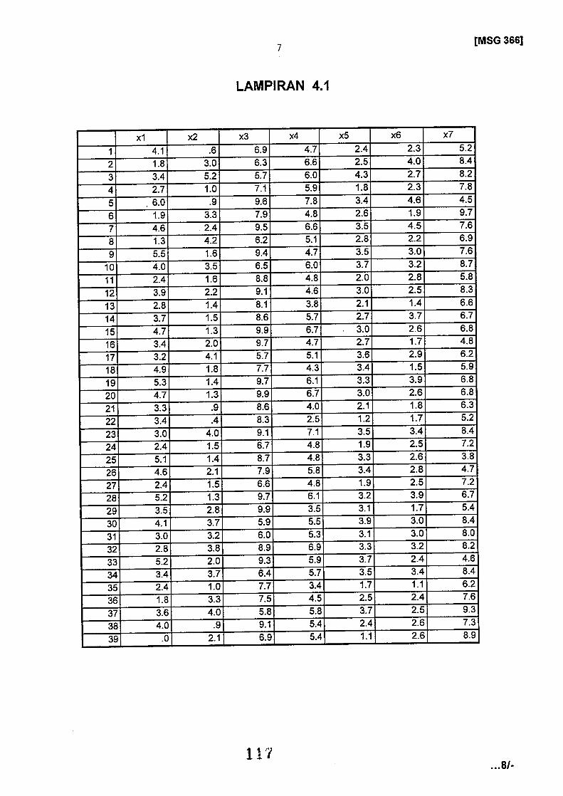
Berbagai teknik multivariat digunakan untuk menganalisa data kajian ini .Lampiran 4.1 memaparkan sebahagian data yang dikutip . Berikut adalah output-output dari perisian statistik (Sila rujuk kepada Lampiran 4.2, 4 .3 dan 4.4.) .Huraikan tujuan penggunaan teknik multivariat dalam setiap output yangdipaparkan dan tafsirkan keputusan-keputusan yang diperoleh . Apakahkesimpulan-kesimpulan anda?

[100 markah]

7

LAMPIRAN 4.1

[MSG 366]

x1 x2 x3 x4 x5 x6 x7

1 4.1 .6 6.9 4.7 2.4 2.3 5.2

2 1 .8 3.0 6.3 6.6 2.5 4.0 8.4

3 3.4 5.2 5.7 6.0 4.3 2.7 8.2

4 2.7 1 .0 7.1 5.9 1 .8 2.3 7.8

5 6.0 .9 9.6 7.8 3.4 4.6 4.5

6 1 .9 3.3 7.9 4.8 2.6 1 .9 9.7

7 4.6 2.4 9.5 6.6 3.5 4.5 7 .6

8 1 .3 4.2 6.2 5.1 2.8 2.2 6.9

9 5.5 1 .6 9.4 4.7 3.5 3.0 7.6

10 4.0 3.5 6.5 6.0 3.7 3.2 8.7

11 2.4 1 .6 8.8 4.8 2.0 2.8 5.8

12 3.9 2.2 9.1 4.6 3.0 2.5 8.3

13 2.8 1 .4 8.1 3.8 2.1 1 .4 6.6

14. 3.7 1 .5 8.6 5.7 2.7 3.7 6.7

15 4.7 1 .3 9.9 6.7 . 3.0 2.6 6.8

16 3.4 2.0 9.7 4.7 2.7 1 .7 4.8

17 3.2 4.1 5.7 5.1 3.6 2.9 6.2

1 8 4.9 1 .8 7.7 4.3 3.4 1 .5 5.9

19 5.3 1 .4 9.7 6.1 3.3 3.9 6.8

20 4.7 1 .3 9.9 6.7 3.0 2.6 6.8

21 3.3 .9 8.6 4.0 2.1 1 .8 6.3

22 3.4 .4 8.3 2.5 1 .2 1 .7 5.2

23 3.0 4.0 9.1 7.1 3.5 3.4 8.4

24 2.4 1 .5 6.7 4.8 1 .9 2.5 7.2

25 5.1 1 .4 8.7 4.8 3.3 2.6 3.8

26 4.6 2.1 7.9 5.8 3.4 2.8 4.7

27 2.4 1 .5 6.6 4.8 1 .9 2.5 7 .2

28 5.2 1 .3 9.7 6.1 3.2 3.9 6.7

29 3.5 2.8 9.9 3.5 3.1 1 .7 5.4

30 4.1 3.7 5.9 5.5 3.9 3.0 8.4

31 3.0 3.2 6.0 5.3 3.1 3.0 8.0

32 2.8 3.8 8.9 6 .9 3.3 3.2 8.2

33 5.2 2.0 9.3 5.9 3.7 2.4 4.6

34 3.4 3.7 6.4 5.7 3.5 3.4 8.4

35 2.4 1 .0 7.7 3.4 1 .7 1 .1 6 .2

36 1 .8 3.3 7.5 4.5 2.5 2.4 7.6

37 3.6 4.0 5.8 5.8 3.7 2.5 9.3

38 4.0 .9 9.1 5.4 2.4 2.6 7.3

39 .0 2.1 6.9 5.4 1 .1 2.6 8.9

[MSG 366]

x8 x9 x10 x11 x12 x13 x141 0 32 .0 4.2 1 0 1 12 1 43.0 4.3 0 1 0 13 1 48.0 5.2 0 1 1 24 1 32.0 3.9 0 1 1 15 0 58.0 6.8 1 0 1 36 1 45.0 4.4 0 1 1 27 0 46.0 5.8 1 0 1 18 1 44.0 4.3 0 1 0 29 0 63.0 5.4 1 0 1 3

10 1 54.0 5.4 0 1 0 211 0 32.0 4.3 1 0 0 112 0 47.0 5.0 1 0 1 213 1 39.0 4.4 0 1 0 114 0 38.0 5.0 1 0 1 115 0 54.0 5.9 1 0 0 316 0 49.0 4.7 1 0 0 317 0 38.0 4.4 1 1 1 218 0 40.0 5.6 1 0 0 219 0 54.0 5.9 1 0 1 320 0 55.0 6.0 1 0 0 321 0 41 .0 4.5 1 0 0 222 0 35.0 3.3 1 0 0 123 0 55.0 5.2 1 1 0 324 1 36.0 3.7 0 1 0 125 0 49.0 4.9 1 0 0 226 0 49.0 5.9 1 0 1 327 1 36.0 3.7 0 1 0 128 0 54.0 5.8 1 0 1 329 0 49.0 5.4 1 0 1 330 1 46.0 5.1 0 1 0 231 1 43.0 3.3 0 1 0 132 0 53.0 5.0 1 1 0 333 0 60.0 6.1 1 0 0 334 1 47.3 3.8 0 1 0 135 1 35.0 4.1 0 1 0 136, 1 39.0 3.6 0 1 1 137 1 44.0 4.8 0 1 1 238 0 46.0 5.1 1 0 1 339 1 29.0 3.9 0 1 1 1

Factor Analysis

KMO and Bartlett's Test

Communalities

Extraction Method : Principal Component Analysis .

LAMPIRAN 4.2

Correlation Matrix

[MSG 366]

Initial ExtractionDelivery Speed 1 .000 .884Price Level 1 .000 .895Price Flexibility 1.000 .649Manufacturer Image 1 .000 .885Service 1 .000 .995Salesforce Image 1 .000 .901Product Quality 1 .000 .618

DeliverySeed Price Level

PriceFlexibility

ManufacturerImage Service

SalesforceImage

ProductQualit

Correlation Delivery Speed 1 .000 -.349 .509 .050 .612 .077 -.483

Price Level -.349 1 .000 -.487 .272 .513 .186 .47C

Price Flexibility .509 -.487 1 .000 -.116 .067 -.034 -.448

Manufacturer Image .050 .272 -.116 1 .000 .299 .788 .20C

Service .612 .513 .067 .299 1 .000 .241 -.05°

Salesforce Image .077 .186 -.034 .788 .241 1 .000 .172

Product Quality -.483 .470 -.448 .200 -.055 .177 1 .00(

Sig . (1-tailed) Delivery Speed .000 .000 .309 .000 .223 .00(

Price Level .000 .000 .003 .000 .032 .00(

Price Flexibility .000 .000 .125 .255 .367 .00(

Manufacturer Image .309 .003 .125 .001 .000 .02 :

Service .000 .000 .255 .001 .008 .29'.

Salesforce Image .223 .032 .367 .000 .008 .035

Product Quality .000 .000 .000 .023 .293 .039

Kaiser-Meyer-Olkin Measure of SamplingAdequacy . .446

Bartlett's Test of Approx . Chi-Square 567.541Sphericity df 21

Sig . .000

Extraction Method : Principal Component Analysis .

Scree Plot.o

0 .02

3

4

5

6

Component Number

Component Matrie

Extraction Method : Principal Component Analysis .a . 3 components extracted .

Total Variance Explained

Com onent1 2 3

Delivery Speed -.528 .752 .202

Price Level .792 9.306E-02 .508Price Flexibility -.692 .374 -.173Manufacturer Image .564 .602 -.452Service .186 .779 .595Salesforce Image .492 .604 -.542Product Quality .739 -.270 -5.43E-03

Initial Ei envalues Extraction Sums of S-~- Rotation Sums of S " uar

Component Total % of Variance Cumulative % Total % of Variance Cumulative % Total % of Variance

1 2.526 36.082 36.082 2.526 36.082 36.082 2.379 33.984

2 2.120 30.291 66.374 2.120 30.291 66.374 1.827 26.098

3 1 .181 16.873 83.246 1 .181 16.873 83.246 1 .622 23.165

4 .541 7.731 90.9775 .418 5.972 96.9496 .204 2.920 99.869

7 9.161 E-03 .131 100.000

Rotated Component Matn*

Extraction Method: Principal Component Analysis .Rotation Method : Varimax with Kaiser Normalization .

a . Rotation converged in 5 iterations .

Component Transformation Matrix

Extraction Method : Principal Component Analysis .Rotation Method : Varimax with Kaiser Normalization .

Component Plot in Rotated Space

.5

or~ponent 2

0.0

rr®1

product Qugmjeole

rrtaagge

el servicee

dernrer~ speedprice flordbility

Olt:1 .0

Component 1

Component 3

Component1 2 3

Delivery Speed -.752 7.112E-02 .560Price Level .754 .108 .561Price Flexibility -.806 6.298E-03 9.531 E-03Manufacturer Image .117 .921 .153Service -6.20E-02 .176 .980Salesforce Image 3.413E-02 .945 7.656E-02Product Quality .760 .193 -6.44E-02

Component 1 2 31 .865 .477 .1592 -.452 .602 .6583 .218 -.641 .736

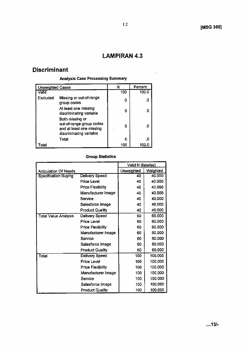
Discriminant

1 2

LAMPIRAN 4.3

Analysis Case Processing Summary

Group Statistics

Unwei hted Cases N PercentValid 100 100.0Excluded Missing or out-of-range 0 .0group codes

At least one missing 0 .0discriminating variableBoth missing orout-of-range group codes 0 .0and at least one missingdiscriminating variableTotal 0 .0

Total 100 100.0

Valid N I stwiseArticulation Of Needs Unwei hted WeightedSpecification Buying Delivery Speed 40 40.000

Price Level 40 40.000Price Flexibility 40 40.000Manufacturer Image 40 40.000Service 40 40.000Salesforce Image 40 40.000Product Quality 40 40.000

Total Value Analysis Delivery Speed 60 60.000Price Level 60 60.000Price Flexibility 60 60.000Manufacturer Image 60 60.000Service 60 60.000Salesforce Image 60 60.000Product Quality 60 60.000

Total Delivery Speed 100 100.000Price Level 100 100.000Price Flexibility 100 100.000Manufacturer Image 100 100.000Service 100 100.000Salesforce Image 100 100.000Product Quality 100 100.000

Test Results

Box's M

73.276F Approx. 2.406

df1

28df2 24453.161Sig . .000

1 3

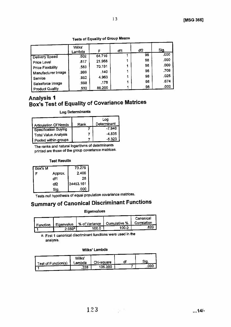
Tests of Equality of Group Means

Analysis 1Box's Test of Equality of Covariance Matrices

Log Determinants

The ranks and natural logarithms of determinantsprinted are those of the group covariance matrices .

Tests null hypothesis of equal population covariance matrices .

Summary of Canonical Discriminant FunctionsEigenvalues

a . First 1 canonical discriminant functions were used in theanalysis.

Wilks' Lambda

[MSG 366]

Wilks'Lambda F df1 df2 Sig .

Delivery Speed .602 64.716 1 98 .000

Price Level .817 21 .968 1 98 .000

Price Flexibility .583 70.191 1 98 .000

Manufacturer Image .999 .140 1 98 .709

Service .952 4.963 1 98 .028

Salesforce Image .998 .178 1 98 .674

Product Quality .532 86.200 1 98 .000

LogArticulation of Needs Rank DeterminantSpecification Buying 7 -7.940

Total Value Analysis 7 -4.835

Pooled within-groups 7 -5.323

Canonical

Function Ei envalue % ofVariance Cumulative % Correlation

1 2.050- 100.0 100.0 .820

Wilks'Test of Functions Lambda Chi-s uare df Sig .1 .328 105.380 7 .000

Standardized Canonical Discriminant Function Coefficients

Structure Matrix

Pooled within-groups correlations between discriminatingvariables and standardized canonical discriminant functionsVariables ordered by absolute size of correlation within function .

Functions at Group Centroids

Unstandardized canonical discriminantfunctions evaluated at group means

Classification StatisticsClassification Processing Summary

1 4

Function1

Delivery Speed .627Price Level .259Price Flexibility .539Manufacturer Image -.064Service -.316Salesforce Image .295Product Quality -.688

Function1

Product Quality -.655Price Flexibility .591Delivery Speed .568Price Level -.331Service .157Salesforce Image .030Manufacturer Image -.026

FunctionArticulation Of Needs 1Specification BuyingTotal Value Analysis

-1 .7361 .157

Processed 100Excluded Missing or out-of-range

group codes0

At least one missing 0discriminating variable

Used in Output 100

Prior Probabilities for Groups

1 5

Classification Function Coefficients

Fisher's linear discriminant functions

Classification Results?

a. 89.0% of original grouped cases correctly classified .

[MSG 366]

Cases Used in Analysis

Articulation Of Needs Prior Unwei hted WeightedSpecification Buying .500 40 40.000

Total Value Analysis .500 60 60.000

Total 1 .000 100 100.000

Articulation Of NeedsSpecification Total Value

Buying AnalysisDelivery Speed 10.077 11 .837Price Level 11 .178 11 .867Price Flexibility 7.154 8.619Manufacturer Image 5.084 4.920

Service -16.775 -18.017Salesforce Image -3.531 -2.428Product Quality 5.114 3.402

(Constant) -61 .586 -66.657

Predicted GroupMembershi

Specification Total ValueArticulation Of Needs Buying Analysis Total

Original Count Specification Buying 38 2 40

Total Value Analysis 9 51 60

% Specification Buying 95.0 5.0 100.0

Total Value Analysis 15.0 85.0 100.0

General Linear ModelBetween-Subjects Factors

Box's Test of Equality of Covariance Matrices

Box's M

9.796F I 1 .584df1

6df2 229276.4Sig . .147Tests the null hypothesis that the observed covariancematrices of the dependent variables are equal across groups .

a. Design : Intercept+X14

Bartletrs Test of Sphericitf

Tests the null hypothesis that the residual covariancematrix is proportional to an identity matrix .

a. Design : Intercept+X14

1 6

LAMPIRAN 4.4

Descriptive Statistics

[MSG 366]

Value Label NType of Buying 1 New Task 34Situation 2 Modified

Rebuy 32

3 StraightRebu 34

Type of Buying Situation Mean Std . Deviation NUsage Level New Task 36.912 5.0595 34

Modified Rebuy 46.531 5.3036 32Straight Rebuy 54.882 4.8727 34Total 46.100 8.9888 100

Satisfaction Level New Task 3.929 .5312 34Modified Rebuy 5.003 .4869 32Straight Rebuy 5.394 .7135 34Total 4.771 .8556 100

Likelihood Ratio .000Approx . Chi-Square 293.124df 2Sig . .000

a . Computed using alpha = .05b . R Squared = .687 (Adjusted R Squared = .681)

c . R Squared = .538 (Adjusted R Squared = .529)

1 7

Levene's Test of Equality of Error Variances

Tests the null hypothesis that the error variance ofthe dependentvariable is equal across groups .

a . Design : Intercept+X14

Multivariate Testsd

a . Computed using alpha = .05b . Exact statisticc . The statistic is an upper bound on F that yields a lower bound on the significance level .

d . Design : Intercept+X14

Tests of Between-Subjects Effects

[MSG 366]

Effect Value F H othesis df Error df Sia .Partial EtaSwared

Intercept Pillai's Trace .992 5634.870 2.000 96.000 .000 .992

Wilks' Lambda .008 5634.870b 2.000 96.000 .000 .992

Hotelling's Trace 117.393 5634.870b 2.000 96.000 .000 .992

Roy's Largest Root 117.393 5634.870b 2.000 96.000 .000 .992

X14 Pillai's Trace .771 30.419 4.000 194.000 .000 .385

Wilks' Lambda .264 45.411b 4.000 192.000 .000 .486

Hotelling's Trace 2.655 63.052 4.000 190.000 .000 .570

Roy's Largest Root 2.604 126.293 2.000 97.000 .000 .723

Type III SumSource Dependent Variable of Squares df Mean Square F Si . .Corrected Model Usage Level 5498.767 2 2749.383 106.666 .000

Satisfaction Level 39.007° 2 19.503 56.542 .000

Intercept Usage Level 212425.420 1 212425.420 8241 .337 .000

Satisfaction Level 2278.727 1 2278.727 6606.172 .000

X14 Usage Level 5498.767 2 2749.383 106.666 .000Satisfaction Level 39.007 2 19.503 56.542 .000

Error Usage Level 2500.233 97 25.776Satisfaction Level 33.459 97 .345

Total Usage Level 220520.000 100Satisfaction Level 2348.710 100

Corrected Total Usage Level 7999.000 99Satisfaction Level 72.466 99

F df1 df2 Sig .Usage LevelSatisfaction Level

.0563.302

22

9797

.945

.041

a . Computed using alpha = .05b . This parameter is set to zero because it is redundant.

Based on Type I II Sum of Squares

1 8

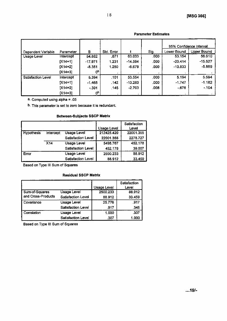
Between-Subjects SSCP Matrix

Based on Type III Sum of Squares

Residual SSCP Matrix

Parameter Estimates

[MSG 366)

95% Confidence Interval

-Dependent Variable Parameter B Std . Error t Sig . Lower Bound Upper BoundUsage Level Intercept 54.882 .871 63.033 .000 53.154 56.610

[X14=1] -17.971 1 .231 -14.594 .000 -20.414 -15.527[X14=2] -8.351 1 .250 -6.679 .000 -10.833 -5.869[X14=3] Ob

Satisfaction Level Intercept 5.394 .101 53.554 .000 5.194 5.594[X14=1] -1 .465 .142 -10.283 .000 -1 .747 -1 .182[X14=2] -.391 .145 -2.703 .008 -.678 -.104[X14=3] O b

SatisfactionUsage Level Level

Hypothesis Intercept Usage Level 212425.420 22001 .355Satisfaction Level 22001 .355 2278.727

X14 Usage Level 5498.767 452.178Satisfaction Level 452.178 39.007

Error Usage Level 2500.233 88.912Satisfaction Level 88.912 33.459

SatisfactionUsage Level Level

Sum-of-Squares Usage Level 2500.233 88.912and Cross-Products Satisfaction Level 88.912 33.459Covariance Usage Level 25.776 .917

Satisfaction Level .917 .345Correlation Usage Level 1 .000 .307

Satisfaction Level .307 1 .000

Tatatanda adalah seperti di dalam kuliah .

1 .

Penguraian spektrum bagi suatu matriks simetrik k x k, A

diberikan oleh

di mana A1, A2' . . ., Ak

adalah

nilai-nilai eigen A dan

ek adalah vektor-vektor eigen terpiauai yange ,1

berkaitan .

1 9Lampiran

[MSG 366]

A = a l e l e' + a2 e 2 e2 + . . . + Ak e k ek

2 .

Katakan X mempunyai E(X) = p- dan Kov (X) = E .

Maka

c'X mempunyai min, c'p dan varians . c'X c .

3 .

f . k . k .

normal bivariat :

f(x x ) =

1

x

exp

11

2

-p 2

)2a `1122(1_P212)

2(1-p12

2x l

_pl

+

x2_

pz

_

P

Ix I - A

x2_p2

2i

12

Q1 22

4 .

f.k.k. normal multivariat :

f (x)

=

1.-

(2w)p/2 e

2

-(1/2)(X

-

p)'E-1 (x

-

p)

5 .

Jika X - N P (p , E) , maka AX - Nq (Aw , A E A' ) .

6 .

Satu sampe 1 :

X n

T2

7 .

Dua sampel tak bersandar :

20Lampiran

(a) T2 = n (X - g)' S-1 (X -

1

E (X ) - X)

1(X - X)'n-1 S=1 ..

2 -1(b)

Lambda uilks

A2/n= ~£+ / IEp

l=

C1+ (nr1))

(c) Selang keyakinan serentak 100(1-a)% bagi C'p

L' X t

P(n-1) F

(a) r'S !'n(n-p) P~n-P

a

S 1fX i+ t

o-1 2P

n.

(d) Selang keyakinan serentak Bonferroni 100(1-a)V. bagi

p i t 1=1, . . .,P :

(a) T2 =L1 - X2 - (u1

u2),, [(n1 + n2 )sPl-1

n1+

n2- 2 P

nl +n2 -p-1 FP .

[MSG 366]

(c)

17I2=

12!1

+

1.122

+

.

.

.

+

Pi2

tn

1 .

2 .

.

.

.

,

p .

TI1

=

h2i

+

VI II

=

1 .

.2 .

. .

.

p .

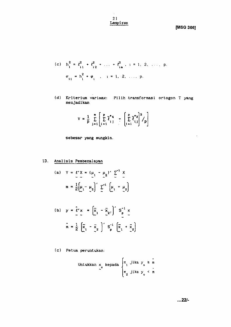
(d) Kriterium varimax: Pilih transformasi ortogon T yangmenjad ikan

sebesar yang mungkin.

13 . Analisis Pembezalayan

(a)

Y =

l'X =

(gl

-

u2 )'

E-1

X

m

(b) y =

m =

1

m

P

*4

P ~*212

V_pE E eIJ - EC I.J /p

2L41-

}12)

E 1

L-

4 1 + u2

Vx =

21Lampiran

2 L1 - x2 J, Sp1 L1 + x2

(c) Petua peruntukan :

- .x

)

.

s-1x

1 2{ PLX

Untukkan x kepada IITIjika yo

m0

Iit2 jika yo< m

[MSG 366]

(b) Seiang keyakinan serentak 100(1-a)% bagi

Q' (p t -

/t2 ) :

8 .

MANOVA satu-hala :

n Q9

- E El LQj XQf=1 J =

n

(b) Seiang keyakinan serentak 100(.1-a)'/, bagi z ky - tQi .

_ +

a

WXkl

X It

t o-9 Pg(g-1)

fi

1 + 1

,,~ nn-g C n

k

n,Qt = 1, 2, . . , p , Q < k -- 1, 2, . . . . 8

9 .

Andaikan

E

mempunyai

d. k .

mEdan

H

mempunyai

d . k .

mH .

IELKatakan A = (E + H

22Lampiran

I , Lit

X2J

±

c

~ ~T1

LX tj)

_1 Sn2

-P

n + n . 2 Pdi mana c2 =

t

2

F

n

+

n2_ .

P _

1

P .

nt,

t

Q

n -2

P

[MSG 366]

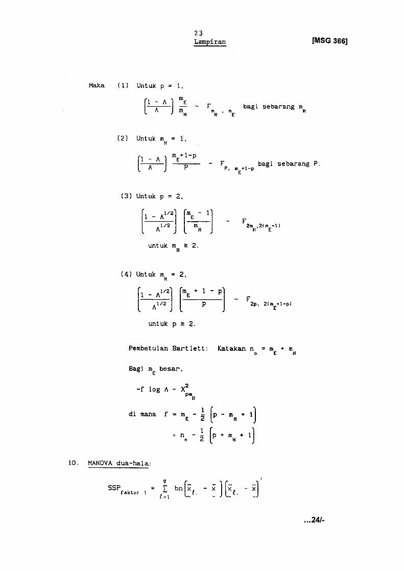
Maka

(1) Untuk p = 1,

10 . MANOVA dues-hales :

~

1

-

A_)

mE-A m

H

(2) Untuk m =H

I1 - A

)

mE+1-p

A

P

Fp,

m .1-

bagi

sebarang P .E p

(3) Untuk p = 2,

untuk m

>_ 2.H

(4) Untuk mH= 2,

1 - A1/2 IME + 1 - pF

A1/2

p

2p, 2(ME+1-p)

untuk p >_ 2 .

Pembetulan Bartlett : Katakan n = m + mo E H

Bag i mE besar .

mE

-f log A - X2pmH

23Lampiran

mH

F

dimanaf=mE-2 (P-mH+1J

n _2 Ip+MH+ lI

Fm 'm

bagi sebarang mHH E

9SSPEaktor

1

-

~1

bn

f.

x

xle= IX

2mH ,2(mE-1)

[MSG 366]

12 . Analisis Faktor

(a) X - . A

11 . Komponen Prinsipal

(a) Y i = e' X ,

i = 1 . 2, . . ,. p . .

kk

pY1,Zk=

e ki

+ i .k = 1 . 2 . . . ., P .

= L F + e

(b) Kov(X) = L L' +

Kov (X ,F) = L

24Lampiran

[MSG 366]

- 000 0 000 -

kr X ek

11 X ekr

Xek

bSSP = E gn -faktor 2 .kk=1

g bSSP

- E E n IXtktindakan

t=1 k=1bersalinq

Xek - X e .

9 b nSSP Eresidual

e=1 k=1 r=1