ORIGINAL RESEARCH ARTICLE

The relationship between Suspended ParticulateMatter and Turbidity at a mooring station in a coastalenvironment: consequences for satellite-derivedproducts

Madihah Jafar-Sidik a,b,*, Francis Gohin c,**, David Bowers b, John Howarth d,Tom Hull e

aBorneo Marine Research Institute, Universiti Malaysia Sabah, Kota Kinabalu, Malaysiab School of Ocean Sciences, Bangor University, Anglesey, United Kingdomc Ifremer, Dyneco/Pelagos, Centre Ifremer de Brest, Plouzane, FrancedNational Oceanography Centre, Joseph Proudman Building, Liverpool, United KingdomeCentre for Environment, Fisheries and Aquaculture Science (Cefas), Lowestoft, United Kingdom

Received 3 February 2017; accepted 7 April 2017Available online 26 April 2017

Oceanologia (2017) 59, 365—378

KEYWORDSTurbidity;Suspended matter;MODIS;Irish Sea

Summary From a data set of observations of Suspended Particulate Matter (SPM) concentra-tion, Turbidity in Formazin Turbidity Unit (FTU) and fluorescence-derived chlorophyll-a at amooring station in Liverpool Bay, in the Irish Sea, we investigate the seasonal variation of the SPM:Turbidity ratio. This ratio changes from a value of around 1 in winter (minimum in January—February) to 2 in summer (maximum in May—June). This seasonal change can be understood interms of the cycle of turbulence and of the phytoplankton population that affects the nature,shape and size of the particles responsible for the Turbidity. The data suggest a direct effect of

Peer review under the responsibility of Institute of Oceanology of the Polish Academy of Sciences.

* Corresponding author at: Borneo Marine Research Institute, Universiti Malaysia Sabah, 88450 Kota Kinabalu, Sabah, Malaysia.Tel.: +60 88320000x2600; fax: +60 88320261.** Corresponding author at: Ifremer, Dyneco/Pelagos, Centre Ifremer de Brest, BP 70, F-29280 Plouzane, Brittany, France. Tel.: +33 298224315;fax: +33 298224548.

E-mail addresses: madihahjsm@gmail.com (M. Jafar-Sidik), Francis.Gohin@ifremer.fr (F. Gohin), d.g.bowers@bangor.ac.uk (D. Bowers),mjh@noc.ac.uk (J. Howarth), tom.hull@cefas.co.uk (T. Hull).

Available online at www.sciencedirect.com

ScienceDirect

j our na l h omepa g e: www.j ou rn al s . els ev ie r. com/oc ea nol og ia /

http://dx.doi.org/10.1016/j.oceano.2017.04.0030078-3234/© 2017 The Authors. Production and hosting by Elsevier Sp. z o.o. on behalf of Institute of Oceanology of the Polish Academy of

Sciences. This is an open access article under the CC BY-NC-ND license (http://creativecommons.org/licenses/by-nc-nd/4.0/).

phytoplankton on the SPM:Turbidity ratio during the spring bloom occurring in April and May and adelayed effect, likely due to aggregation of particles, in July and August. Based on the hypothesisthat only SPM concentration varies, but not the mass-specific backscattering coefficient ofparticles bbp

*, semi-analytical algorithms aiming at retrieving SPM from satellite radiance ignorethe seasonal variability of bbp

* which is likely to be inversely correlated to the SPM:Turbidity ratio.A simple sinusoidal modulation of the relationship between Turbidity and SPM with time helps tocorrect this effect at the location of the mooring. Without applying a seasonal modulation to bbp

*,there is an underestimation of SPM in summer by the Ifremer semi-analytical algorithm (Gohinet al., 2015) we tested. SPM derived from this algorithm, as expected from any semi-analyticalalgorithm, appears to be more related to in situ Turbidity than to in situ SPM throughout the year.© 2017 The Authors. Production and hosting by Elsevier Sp. z o.o. on behalf of Institute ofOceanology of the Polish Academy of Sciences. This is an open access article under the CC BY-NC-ND license (http://creativecommons.org/licenses/by-nc-nd/4.0/).

366 M. Jafar-Sidik et al./Oceanologia 59 (2017) 365—378

1. Introduction

Suspended Particulate Matter (SPM) is a major component ofthe coastal environment that is monitored for multiple pur-poses. We may name among them a better knowledge ofsediment transport and the response of the suspended sedi-ment load to resuspension, deposition, and river discharge.Through light absorption and scattering the SPM also contri-butes to water clarity and governs the amount of photonsavailable for photosynthesis in the water column. Suspendedmatter is also a state variable of the sediment transport andbiogeochemical models of coastal seas. The geographical dis-tribution of SPM concentration is key for analyzing the deposi-tion and erosion patterns in an estuary and evaluating thematerial fluxes from river to sea. Satellite remote-sensing,associated with instrumented moorings, provide useful datafor investigating the spatial and temporal variation of SPM inestuarial and coastal zones. Some of these algorithms (Bindinget al., 2003; Forget et al., 1999; Lahet et al., 2000; Li et al.,1998) are empirical and others (Eleveld et al., 2008; Gohinet al., 2005; Han et al., 2016; Nechad et al., 2010; Van derWoerd and Pasterkamp, 2008) are semi-analytical as they makeuse of the Inherent Optical Properties (IOPs) of the waterconstituents. Products of non-algal SPM derived from theIfremer semi-analytical algorithm (Gohin et al., 2005; Gohin,2011) have been provided for years to a large community andused, with or without in situ data, for validating hydro-sedi-mentary models (Edwards et al., 2012; Ford et al., 2017;Guillou et al., 2015, 2016; Ménésguen and Gohin, 2006; Sykesand Barciela, 2012; Van der Molen et al., 2016, 2017) or forcingthe light component in biogeochemical modelling (Huret et al.,2007) over the northwest European continental shelf.

Autonomous observation platforms such as ferrybox orinstrumented buoys typically do not provide SPM concentra-tion directly but instead provide Turbidity measurements.Turbidity data are by far the most frequent data set related toSPM provided to the scientific community and managers ofthe coastal environment. For this reason and as Turbidity istightly related to backscattering, Dogliotti et al. (2015)suggest making use of a semi-analytical relation to estimateTurbidity from marine reflectance and, in a second step,derive SPM from Turbidity. All semi-analytical methods aim-ing to retrieve directly SPM concentration assume thestability of the mass-specific backscattering, bbp

*, which isconsidered as constant in space and throughout the seasons.This assumption remains to be verified in coastal waters

where there is a seasonal variation in the nature of theSPM, from small mineral particles in winter to phytoplanktoncells, aggregates and flocs in summer.

Martinez-Vicente et al. (2010) observed a seasonal effecton the scattering properties of particles at a coastal stationof the Western English Channel (the L4 station located offPlymouth at 50.25N, 4.22W). These authors observed thatthe SPM:bp(555) ratio (where bp is the scattering coefficientof mineral and organic particles) varies between a wintermean of 2 and a summer mean of 1.1 g m�2. The mean mass-specific particle backscattering coefficient, bbp

* was0.0027 m2 g�1 for total SPM at 532 nm, and higher withrespect to Suspended Particulate Inorganic Matter (SPIM).The measured mass-specific backscattering, bbp

*, was0.0075 in winter and 0.0023 m2 g�1 in summer; which is atthe lower end of values reported for coastal waters (Berthonet al., 2007; Snyder et al., 2008). Given the small amount ofdata available, however, the authors recognised that it wasdifficult to draw conclusions about the seasonality of thiscoefficient. At the L4 station, the SPM mean value wasrelatively low for a coastal site (1.00 � 0.88 g m�3) withpeaks in winter (with a stronger contribution of SPIM). How-ever, the highest winter peak of 9.94 g m�3 is lower than thatobserved in general in coastal waters (up to 100 g m�3 inwinter). A particularly high content of mineral particles inwinter and strong phytoplankton blooms in summer are likelyto emphasise the variability of the inorganic:organic fractionfor suspended particles in coastal waters with consequencesfor the backscattering properties.

In a study encompassing a large range of water types,Neukermans et al. (2012) observed that waters dominated bymineral particles backscatter up to 2.4 times more per unitmass, bbp

* = 0.0121 m2 g�1, than waters dominated byorganic particles, bbp

* = 0.0051 m2 g�1 at 650 nm. Similarconclusions were pointed out in Arctic seawaters by Reynoldset al. (2016) who observed that the average bbp

* of mineralassemblages was almost twice that of organic assemblages.The positive dependency of the mass-specific backscatteringcoefficient on the SPIM:SPM ratio has also been shown byBowers et al. (2014).

In the Irish Sea, McKee and Cunningham (2006) identifiedtwo water sub-types that are distinguished both optically andby the ratio of the concentrations of their constituents (Chl:SPIM). The Inherent Optical Properties (IOPs) at stations witha low ratio of chlorophyll-a to suspended particles, Group“Mineral”, were highly correlated with the concentration of

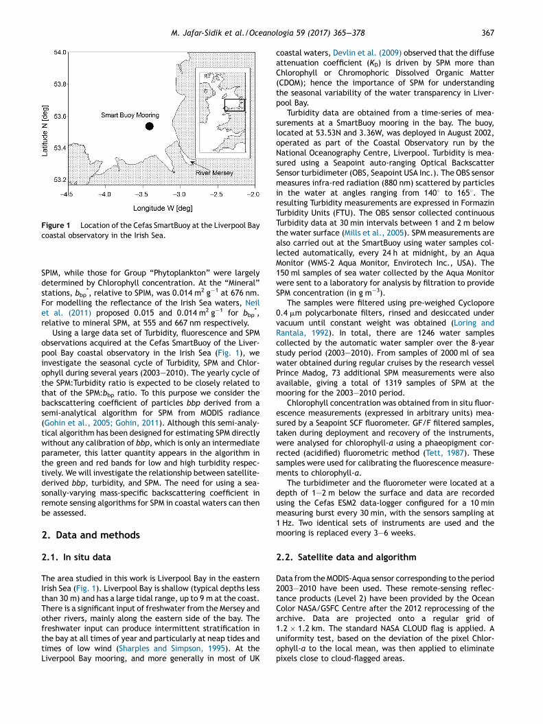
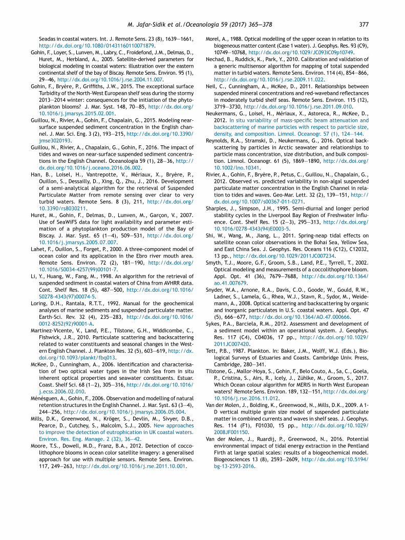
Figure 1 Location of the Cefas SmartBuoy at the Liverpool Baycoastal observatory in the Irish Sea.

M. Jafar-Sidik et al./Oceanologia 59 (2017) 365—378 367

SPIM, while those for Group “Phytoplankton” were largelydetermined by Chlorophyll concentration. At the “Mineral”stations, bbp

*, relative to SPIM, was 0.014 m2 g�1 at 676 nm.For modelling the reflectance of the Irish Sea waters, Neilet al. (2011) proposed 0.015 and 0.014 m2 g�1 for bbp

*,relative to mineral SPM, at 555 and 667 nm respectively.

Using a large data set of Turbidity, fluorescence and SPMobservations acquired at the Cefas SmartBuoy of the Liver-pool Bay coastal observatory in the Irish Sea (Fig. 1), weinvestigate the seasonal cycle of Turbidity, SPM and Chlor-ophyll during several years (2003—2010). The yearly cycle ofthe SPM:Turbidity ratio is expected to be closely related tothat of the SPM:bbp ratio. To this purpose we consider thebackscattering coefficient of particles bbp derived from asemi-analytical algorithm for SPM from MODIS radiance(Gohin et al., 2005; Gohin, 2011). Although this semi-analy-tical algorithm has been designed for estimating SPM directlywithout any calibration of bbp, which is only an intermediateparameter, this latter quantity appears in the algorithm inthe green and red bands for low and high turbidity respec-tively. We will investigate the relationship between satellite-derived bbp, turbidity, and SPM. The need for using a sea-sonally-varying mass-specific backscattering coefficient inremote sensing algorithms for SPM in coastal waters can thenbe assessed.

2. Data and methods

2.1. In situ data

The area studied in this work is Liverpool Bay in the easternIrish Sea (Fig. 1). Liverpool Bay is shallow (typical depths lessthan 30 m) and has a large tidal range, up to 9 m at the coast.There is a significant input of freshwater from the Mersey andother rivers, mainly along the eastern side of the bay. Thefreshwater input can produce intermittent stratification inthe bay at all times of year and particularly at neap tides andtimes of low wind (Sharples and Simpson, 1995). At theLiverpool Bay mooring, and more generally in most of UK

coastal waters, Devlin et al. (2009) observed that the diffuseattenuation coefficient (KD) is driven by SPM more thanChlorophyll or Chromophoric Dissolved Organic Matter(CDOM); hence the importance of SPM for understandingthe seasonal variability of the water transparency in Liver-pool Bay.

Turbidity data are obtained from a time-series of mea-surements at a SmartBuoy mooring in the bay. The buoy,located at 53.53N and 3.36W, was deployed in August 2002,operated as part of the Coastal Observatory run by theNational Oceanography Centre, Liverpool. Turbidity is mea-sured using a Seapoint auto-ranging Optical BackscatterSensor turbidimeter (OBS, Seapoint USA Inc.). The OBS sensormeasures infra-red radiation (880 nm) scattered by particlesin the water at angles ranging from 1408 to 1658. Theresulting Turbidity measurements are expressed in FormazinTurbidity Units (FTU). The OBS sensor collected continuousTurbidity data at 30 min intervals between 1 and 2 m belowthe water surface (Mills et al., 2005). SPM measurements arealso carried out at the SmartBuoy using water samples col-lected automatically, every 24 h at midnight, by an AquaMonitor (WMS-2 Aqua Monitor, Envirotech Inc., USA). The150 ml samples of sea water collected by the Aqua Monitorwere sent to a laboratory for analysis by filtration to provideSPM concentration (in g m�3).

The samples were filtered using pre-weighed Cyclopore0.4 mm polycarbonate filters, rinsed and desiccated undervacuum until constant weight was obtained (Loring andRantala, 1992). In total, there are 1246 water samplescollected by the automatic water sampler over the 8-yearstudy period (2003—2010). From samples of 2000 ml of seawater obtained during regular cruises by the research vesselPrince Madog, 73 additional SPM measurements were alsoavailable, giving a total of 1319 samples of SPM at themooring for the 2003—2010 period.

Chlorophyll concentration was obtained from in situ fluor-escence measurements (expressed in arbitrary units) mea-sured by a Seapoint SCF fluorometer. GF/F filtered samples,taken during deployment and recovery of the instruments,were analysed for chlorophyll-a using a phaeopigment cor-rected (acidified) fluorometric method (Tett, 1987). Thesesamples were used for calibrating the fluorescence measure-ments to chlorophyll-a.

The turbidimeter and the fluorometer were located at adepth of 1—2 m below the surface and data are recordedusing the Cefas ESM2 data-logger configured for a 10 minmeasuring burst every 30 min, with the sensors sampling at1 Hz. Two identical sets of instruments are used and themooring is replaced every 3—6 weeks.

2.2. Satellite data and algorithm

Data from the MODIS-Aqua sensor corresponding to the period2003—2010 have been used. These remote-sensing reflec-tance products (Level 2) have been provided by the OceanColor NASA/GSFC Centre after the 2012 reprocessing of thearchive. Data are projected onto a regular grid of1.2 � 1.2 km. The standard NASA CLOUD flag is applied. Auniformity test, based on the deviation of the pixel Chlor-ophyll-a to the local mean, was then applied to eliminatepixels close to cloud-flagged areas.

368 M. Jafar-Sidik et al./Oceanologia 59 (2017) 365—378

The semi-analytical model used to retrieve non-algal SPMfrom satellite reflectance is described in Gohin et al. (2005)and Gohin (2011). Non-algal SPM (NA_SPM), defined as non-living SPM (not related to Chl) in the 2005 publication, isestimated from radiance at 555 nm and 667 nm after apreliminary estimation of the chlorophyll-a concentrationby the OC5 algorithm (Gohin et al., 2002; Tilstone et al.,2017). Depending on the NA_SPM level retrieved, the finalNA_SPM is chosen at 555 nm if NA_SPM at 555 nm is less than4 g m�3 and NA_SPM at 667 nm less than 3.9 g m�3. This isgenerally the case in relatively clear waters. In other casesNA_SPM (670) is chosen.

The semi-analytical algorithm proceeds in two steps forestimating NA_SPM at 555 nm and 667 nm. In the first step anintermediate term R0 is estimated from the normalisedwater-leaving radiance nLw. The normalised water-leavingradiance, is the light that would exit the ocean with a sun atthe zenith in the absence of an atmosphere and at the meanearth-sun distance. It is obtained by multiplying the remote-sensing reflectance by the extraterrestrial solar irradianceprovided by NASA for each MODIS-Aqua waveband.

R0 ¼ a0 þ a1nLw; (1)

here a0 and a1 are two constants defined for each wavelength(551 and 667 nm).

R0 is related to the backscattering and absorption coeffi-cients by

R0 ¼ bba þ bb

: (2)

In Eq. (2), a and bb are the absorption and backscatteringcoefficients (wavelength-dependent). These coefficients canbe written in terms of the concentration of Chl and SPM asshown in Eq. (3).

a ¼ aw þ a�chl � Chl þ a�nap � NA SPM;bb ¼ bbw þ b�bChl � Chl þ b�bnap � NA SPM; (3)

where the * quantities represent the mass-specific IOPs (ofChl and NA_SPM); w indicates pure water. A specific contri-bution of coloured dissolved organic material (CDOM) toabsorption in these green and red wavelengths is ignoredin the algorithm. Absorption by CDOM associated with thedecay of phytoplankton is accounted for through aChl*.

After making these substitutions, the NA_SPM concentra-tion is then obtained by inverting Eq. (2):

NA SPM ¼ R0x½aw þ bw þ ða�chl þ b�bChlÞ�Chl��½bbw þ b�bChlChl�b�bnap�ða�nap þ b�bnapÞ�R0 :

(4)

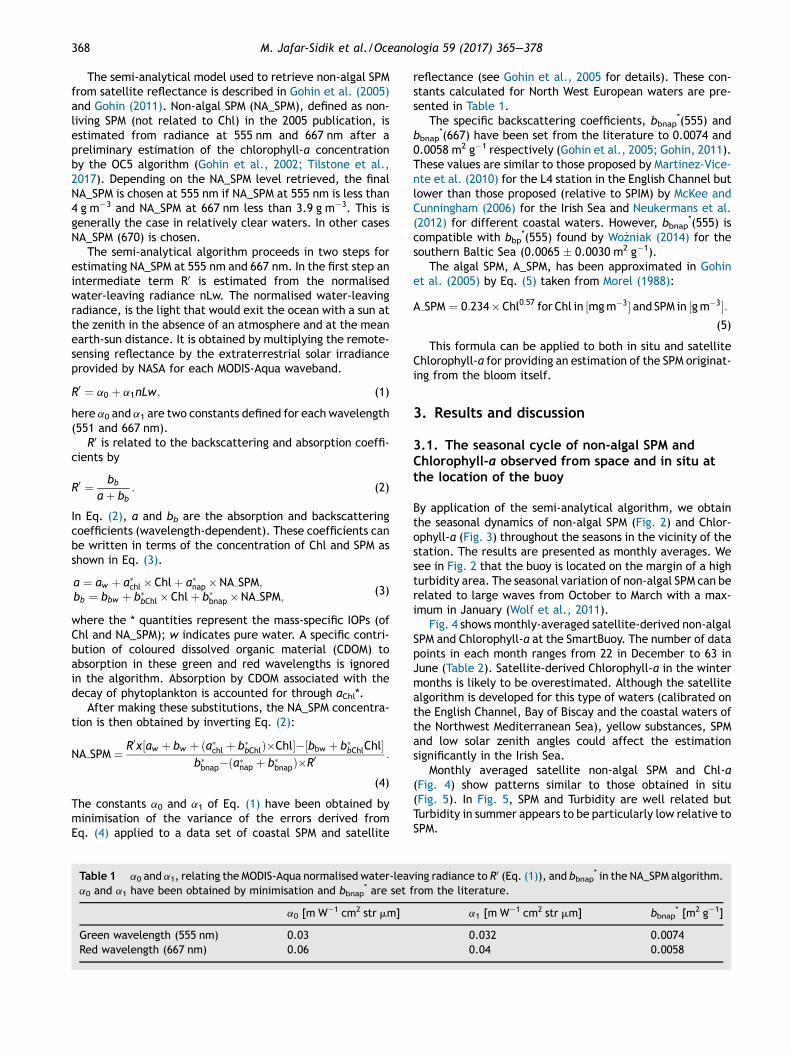
The constants a0 and a1 of Eq. (1) have been obtained byminimisation of the variance of the errors derived fromEq. (4) applied to a data set of coastal SPM and satellite

Table 1 a0 and a1, relating the MODIS-Aqua normalised water-leava0 and a1 have been obtained by minimisation and bbnap

* are set f

a0 [m W�1 cm2 str mm]

Green wavelength (555 nm) 0.03

Red wavelength (667 nm) 0.06

reflectance (see Gohin et al., 2005 for details). These con-stants calculated for North West European waters are pre-sented in Table 1.

The specific backscattering coefficients, bbnap*(555) and

bbnap*(667) have been set from the literature to 0.0074 and

0.0058 m2 g�1 respectively (Gohin et al., 2005; Gohin, 2011).These values are similar to those proposed by Martinez-Vice-nte et al. (2010) for the L4 station in the English Channel butlower than those proposed (relative to SPIM) by McKee andCunningham (2006) for the Irish Sea and Neukermans et al.(2012) for different coastal waters. However, bbnap

*(555) iscompatible with bbp

*(555) found by Woźniak (2014) for thesouthern Baltic Sea (0.0065 � 0.0030 m2 g�1).

The algal SPM, A_SPM, has been approximated in Gohinet al. (2005) by Eq. (5) taken from Morel (1988):

A SPM ¼ 0:234 � Chl0:57 for Chl in ½mg m�3� and SPM in ½g m�3�:(5)

This formula can be applied to both in situ and satelliteChlorophyll-a for providing an estimation of the SPM originat-ing from the bloom itself.

3. Results and discussion

3.1. The seasonal cycle of non-algal SPM andChlorophyll-a observed from space and in situ atthe location of the buoy

By application of the semi-analytical algorithm, we obtainthe seasonal dynamics of non-algal SPM (Fig. 2) and Chlor-ophyll-a (Fig. 3) throughout the seasons in the vicinity of thestation. The results are presented as monthly averages. Wesee in Fig. 2 that the buoy is located on the margin of a highturbidity area. The seasonal variation of non-algal SPM can berelated to large waves from October to March with a max-imum in January (Wolf et al., 2011).

Fig. 4 shows monthly-averaged satellite-derived non-algalSPM and Chlorophyll-a at the SmartBuoy. The number of datapoints in each month ranges from 22 in December to 63 inJune (Table 2). Satellite-derived Chlorophyll-a in the wintermonths is likely to be overestimated. Although the satellitealgorithm is developed for this type of waters (calibrated onthe English Channel, Bay of Biscay and the coastal waters ofthe Northwest Mediterranean Sea), yellow substances, SPMand low solar zenith angles could affect the estimationsignificantly in the Irish Sea.

Monthly averaged satellite non-algal SPM and Chl-a(Fig. 4) show patterns similar to those obtained in situ(Fig. 5). In Fig. 5, SPM and Turbidity are well related butTurbidity in summer appears to be particularly low relative toSPM.

ing radiance to R0 (Eq. (1)), and bbnap* in the NA_SPM algorithm.

rom the literature.

a1 [m W�1 cm2 str mm] bbnap* [m2 g�1]

0.032 0.00740.04 0.0058

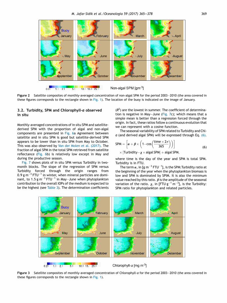
Figure 2 Satellite composites of monthly-averaged concentration of non-algal SPM for the period 2003—2010 (the area covered inthese figures corresponds to the rectangle shown in Fig. 1). The location of the buoy is indicated on the image of January.

M. Jafar-Sidik et al./Oceanologia 59 (2017) 365—378 369

3.2. Turbidity, SPM and Chlorophyll-a observedin situ

Monthly-averaged concentrations of in situ SPM and satellite-derived SPM with the proportion of algal and non-algalcomponents are presented in Fig. 6a Agreement betweensatellite and in situ SPM is good but satellite-derived SPMappears to be lower than in situ SPM from May to October.This was also observed by Van der Molen et al. (2017). Thefraction of algal SPM in the total SPM retrieved from satellitereflectance (Fig. 6b) is relatively low except in May andduring the productive season.

Fig. 7 shows plots of in situ SPM versus Turbidity in two-month blocks. The slope of the regression of SPM versusTurbidity forced through the origin ranges from0.9 g m�3 FTU�1 in winter, when mineral particles are domi-nant, to 1.5 g m�3 FTU�1 in May—June when phytoplanktoncontribution to the overall IOPs of the medium is expected tobe the highest (see Table 3). The determination coefficients

Figure 3 Satellite composites of monthly-averaged concentrationthese figures corresponds to the rectangle shown in Fig. 1).

(R2) are the lowest in summer. The coefficient of determina-tion is negative in May—June (Fig. 7c); which means that asimple mean is better than a regression forced through theorigin. In fact, these ratios follow a continuous evolution thatwe can represent with a cosine function.

The seasonal variability of SPM related to Turbidity and Chl-a (and derived algal SPM) will be expressed through Eq. (6).

SPM ¼ a þ b � 1�costime � 2p

365

� �� �� �

� ½Turbidity�x � algal SPM� þ algal SPM;

(6)

where time is the day of the year and SPM is total SPM.Turbidity is in FTU.

The term a, in [g m�3 FTU�1], is the SPM:Turbidity ratio atthe beginning of the year when the phytoplankton biomass islow and SPM is dominated by SPIM. It is also the minimumvalue reached by this ratio. b is the amplitude of the seasonalvariation of the ratio. x, in [FTU g�1 m�3], is the Turbidity:SPM ratio for phytoplankton and related particles.

of Chlorophyll-a for the period 2003—2010 (the area covered in

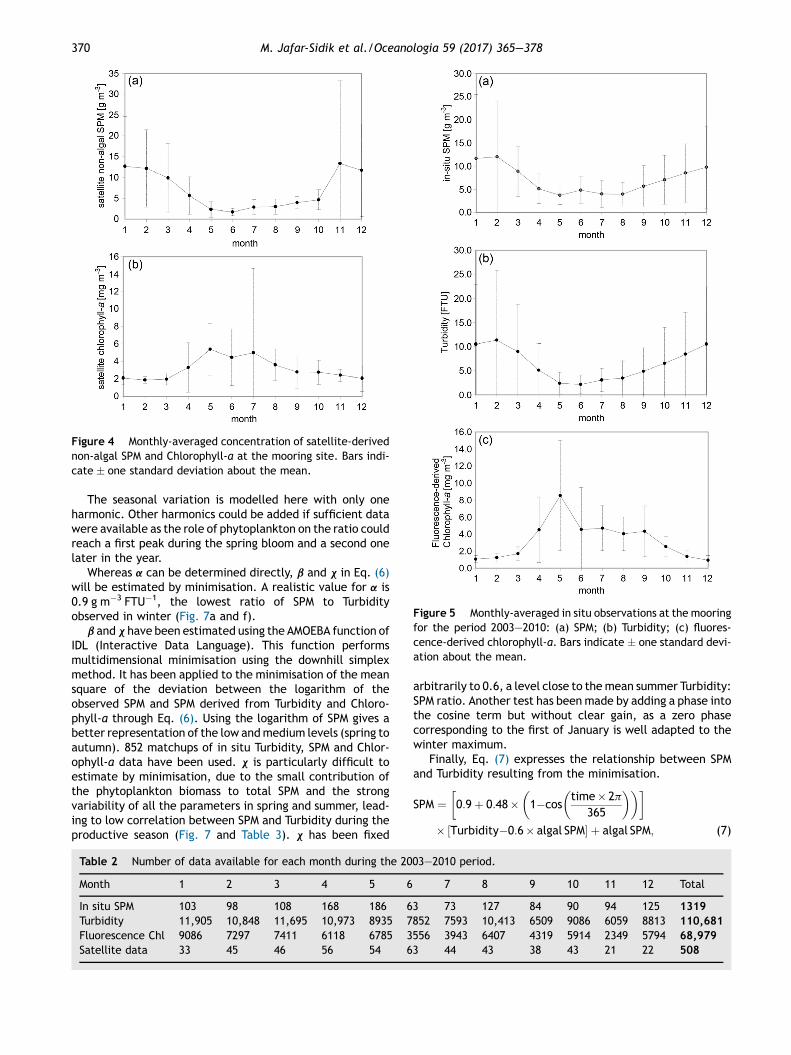
Figure 4 Monthly-averaged concentration of satellite-derivednon-algal SPM and Chlorophyll-a at the mooring site. Bars indi-cate � one standard deviation about the mean.

Figure 5 Monthly-averaged in situ observations at the mooringfor the period 2003—2010: (a) SPM; (b) Turbidity; (c) fluores-cence-derived chlorophyll-a. Bars indicate � one standard devi-ation about the mean.

370 M. Jafar-Sidik et al./Oceanologia 59 (2017) 365—378

The seasonal variation is modelled here with only oneharmonic. Other harmonics could be added if sufficient datawere available as the role of phytoplankton on the ratio couldreach a first peak during the spring bloom and a second onelater in the year.

Whereas a can be determined directly, b and x in Eq. (6)will be estimated by minimisation. A realistic value for a is0.9 g m�3 FTU�1, the lowest ratio of SPM to Turbidityobserved in winter (Fig. 7a and f).

b and x have been estimated using the AMOEBA function ofIDL (Interactive Data Language). This function performsmultidimensional minimisation using the downhill simplexmethod. It has been applied to the minimisation of the meansquare of the deviation between the logarithm of theobserved SPM and SPM derived from Turbidity and Chloro-phyll-a through Eq. (6). Using the logarithm of SPM gives abetter representation of the low and medium levels (spring toautumn). 852 matchups of in situ Turbidity, SPM and Chlor-ophyll-a data have been used. x is particularly difficult toestimate by minimisation, due to the small contribution ofthe phytoplankton biomass to total SPM and the strongvariability of all the parameters in spring and summer, lead-ing to low correlation between SPM and Turbidity during theproductive season (Fig. 7 and Table 3). x has been fixed

Table 2 Number of data available for each month during the 20

Month 1 2 3 4 5 6

In situ SPM 103 98 108 168 186 6Turbidity 11,905 10,848 11,695 10,973 8935 7Fluorescence Chl 9086 7297 7411 6118 6785 3Satellite data 33 45 46 56 54 6

arbitrarily to 0.6, a level close to the mean summer Turbidity:SPM ratio. Another test has been made by adding a phase intothe cosine term but without clear gain, as a zero phasecorresponding to the first of January is well adapted to thewinter maximum.

Finally, Eq. (7) expresses the relationship between SPMand Turbidity resulting from the minimisation.

SPM ¼ 0:9 þ 0:48 � 1�costime � 2p

365

� �� �� �

� ½Turbidity�0:6 � algal SPM� þ algal SPM; (7)

03—2010 period.

7 8 9 10 11 12 Total

3 73 127 84 90 94 125 1319852 7593 10,413 6509 9086 6059 8813 110,681556 3943 6407 4319 5914 2349 5794 68,9793 44 43 38 43 21 22 508

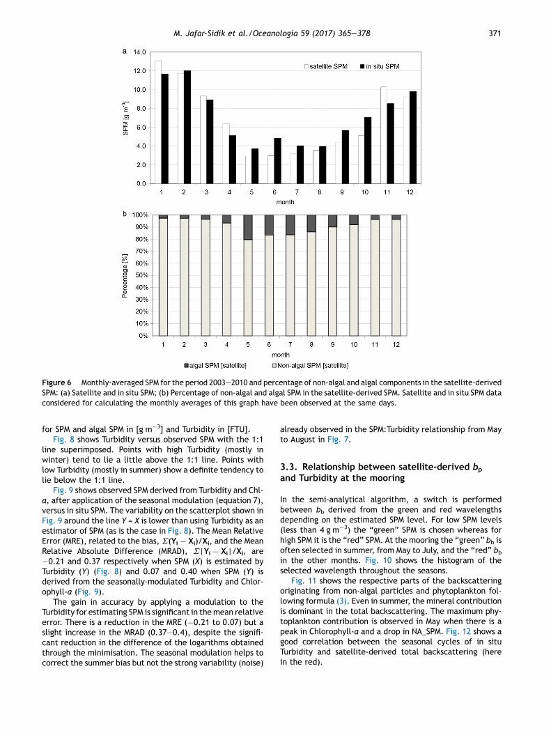
Figure 6 Monthly-averaged SPM for the period 2003—2010 and percentage of non-algal and algal components in the satellite-derivedSPM: (a) Satellite and in situ SPM; (b) Percentage of non-algal and algal SPM in the satellite-derived SPM. Satellite and in situ SPM dataconsidered for calculating the monthly averages of this graph have been observed at the same days.

M. Jafar-Sidik et al./Oceanologia 59 (2017) 365—378 371

for SPM and algal SPM in [g m�3] and Turbidity in [FTU].Fig. 8 shows Turbidity versus observed SPM with the 1:1

line superimposed. Points with high Turbidity (mostly inwinter) tend to lie a little above the 1:1 line. Points withlow Turbidity (mostly in summer) show a definite tendency tolie below the 1:1 line.

Fig. 9 shows observed SPM derived from Turbidity and Chl-a, after application of the seasonal modulation (equation 7),versus in situ SPM. The variability on the scatterplot shown inFig. 9 around the line Y = X is lower than using Turbidity as anestimator of SPM (as is the case in Fig. 8). The Mean RelativeError (MRE), related to the bias, S(Yi � Xi)/Xi, and the MeanRelative Absolute Difference (MRAD), S|Yi � Xi|/Xi, are�0.21 and 0.37 respectively when SPM (X) is estimated byTurbidity (Y) (Fig. 8) and 0.07 and 0.40 when SPM (Y) isderived from the seasonally-modulated Turbidity and Chlor-ophyll-a (Fig. 9).

The gain in accuracy by applying a modulation to theTurbidity for estimating SPM is significant in the mean relativeerror. There is a reduction in the MRE (�0.21 to 0.07) but aslight increase in the MRAD (0.37—0.4), despite the signifi-cant reduction in the difference of the logarithms obtainedthrough the minimisation. The seasonal modulation helps tocorrect the summer bias but not the strong variability (noise)

already observed in the SPM:Turbidity relationship from Mayto August in Fig. 7.

3.3. Relationship between satellite-derived bpand Turbidity at the mooring

In the semi-analytical algorithm, a switch is performedbetween bb derived from the green and red wavelengthsdepending on the estimated SPM level. For low SPM levels(less than 4 g m�3) the “green” SPM is chosen whereas forhigh SPM it is the “red” SPM. At the mooring the “green” bb isoften selected in summer, from May to July, and the “red” bbin the other months. Fig. 10 shows the histogram of theselected wavelength throughout the seasons.

Fig. 11 shows the respective parts of the backscatteringoriginating from non-algal particles and phytoplankton fol-lowing formula (3). Even in summer, the mineral contributionis dominant in the total backscattering. The maximum phy-toplankton contribution is observed in May when there is apeak in Chlorophyll-a and a drop in NA_SPM. Fig. 12 shows agood correlation between the seasonal cycles of in situTurbidity and satellite-derived total backscattering (herein the red).

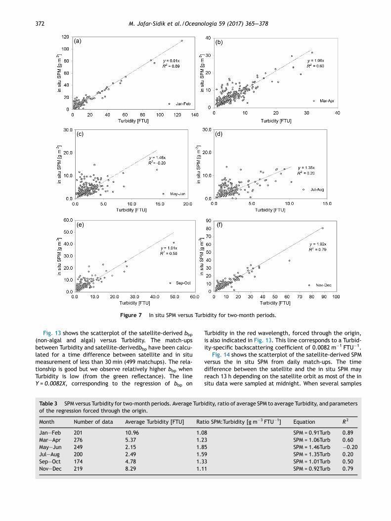
Figure 7 In situ SPM versus Turbidity for two-month periods.

372 M. Jafar-Sidik et al./Oceanologia 59 (2017) 365—378

Fig. 13 shows the scatterplot of the satellite-derived bbp(non-algal and algal) versus Turbidity. The match-upsbetween Turbidity and satellite-derivedbbp have been calcu-lated for a time difference between satellite and in situmeasurement of less than 30 min (499 matchups). The rela-tionship is good but we observe relatively higher bbp whenTurbidity is low (from the green reflectance). The lineY = 0.0082X, corresponding to the regression of bbp on

Table 3 SPM versus Turbidity for two-month periods. Average Turbof the regression forced through the origin.

Month Number of data Average Turbidity [FTU] Ra

Jan—Feb 201 10.96 1.0Mar—Apr 276 5.37 1.2May—Jun 249 2.15 1.8Jul—Aug 200 2.49 1.5Sep—Oct 174 4.78 1.3Nov—Dec 219 8.29 1.1

Turbidity in the red wavelength, forced through the origin,is also indicated in Fig. 13. This line corresponds to a Turbid-ity-specific backscattering coefficient of 0.0082 m�1 FTU�1.

Fig. 14 shows the scatterplot of the satellite-derived SPMversus the in situ SPM from daily match-ups. The timedifference between the satellite and the in situ SPM mayreach 13 h depending on the satellite orbit as most of the insitu data were sampled at midnight. When several samples

idity, ratio of average SPM to average Turbidity, and parameters

tio SPM:Turbidity [g m�3 FTU�1] Equation R 2

8 SPM = 0.91Turb 0.893 SPM = 1.06Turb 0.605 SPM = 1.46Turb �0.209 SPM = 1.35Turb 0.203 SPM = 1.01Turb 0.501 SPM = 0.92Turb 0.79

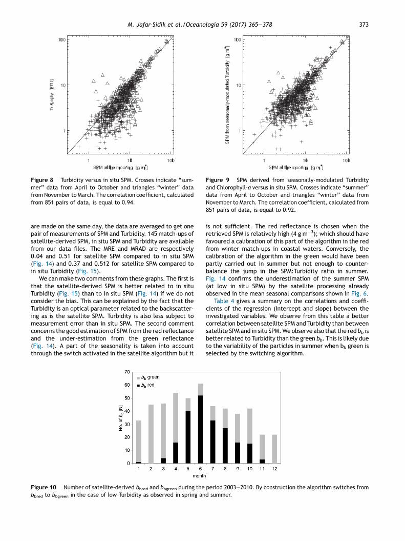
Figure 8 Turbidity versus in situ SPM. Crosses indicate “sum-mer” data from April to October and triangles “winter” datafrom November to March. The correlation coefficient, calculatedfrom 851 pairs of data, is equal to 0.94.

Figure 9 SPM derived from seasonally-modulated Turbidityand Chlorophyll-a versus in situ SPM. Crosses indicate “summer”data from April to October and triangles “winter” data fromNovember to March. The correlation coefficient, calculated from851 pairs of data, is equal to 0.92.

M. Jafar-Sidik et al./Oceanologia 59 (2017) 365—378 373

are made on the same day, the data are averaged to get onepair of measurements of SPM and Turbidity. 145 match-ups ofsatellite-derived SPM, in situ SPM and Turbidity are availablefrom our data files. The MRE and MRAD are respectively0.04 and 0.51 for satellite SPM compared to in situ SPM(Fig. 14) and 0.37 and 0.512 for satellite SPM compared toin situ Turbidity (Fig. 15).

We can make two comments from these graphs. The first isthat the satellite-derived SPM is better related to in situTurbidity (Fig. 15) than to in situ SPM (Fig. 14) if we do notconsider the bias. This can be explained by the fact that theTurbidity is an optical parameter related to the backscatter-ing as is the satellite SPM. Turbidity is also less subject tomeasurement error than in situ SPM. The second commentconcerns the good estimation of SPM from the red reflectanceand the under-estimation from the green reflectance(Fig. 14). A part of the seasonality is taken into accountthrough the switch activated in the satellite algorithm but it

Figure 10 Number of satellite-derived bbred and bbgreen during thebbred to bbgreen in the case of low Turbidity as observed in spring an

is not sufficient. The red reflectance is chosen when theretrieved SPM is relatively high (4 g m�3); which should havefavoured a calibration of this part of the algorithm in the redfrom winter match-ups in coastal waters. Conversely, thecalibration of the algorithm in the green would have beenpartly carried out in summer but not enough to counter-balance the jump in the SPM:Turbidity ratio in summer.Fig. 14 confirms the underestimation of the summer SPM(at low in situ SPM) by the satellite processing alreadyobserved in the mean seasonal comparisons shown in Fig. 6.

Table 4 gives a summary on the correlations and coeffi-cients of the regression (intercept and slope) between theinvestigated variables. We observe from this table a bettercorrelation between satellite SPM and Turbidity than betweensatellite SPM and in situ SPM. We observe also that the red bb isbetter related to Turbidity than the green bb. This is likely dueto the variability of the particles in summer when bb green isselected by the switching algorithm.

period 2003—2010. By construction the algorithm switches fromd summer.

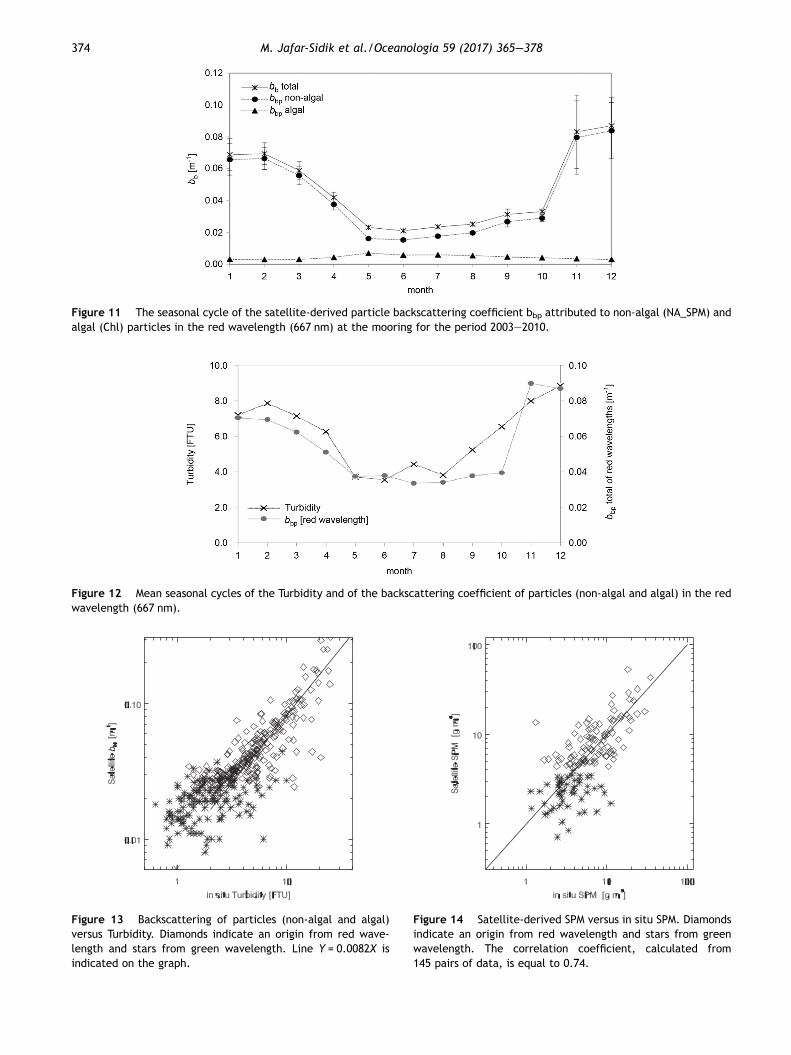
Figure 11 The seasonal cycle of the satellite-derived particle backscattering coefficient bbp attributed to non-algal (NA_SPM) andalgal (Chl) particles in the red wavelength (667 nm) at the mooring for the period 2003—2010.

Figure 12 Mean seasonal cycles of the Turbidity and of the backscattering coefficient of particles (non-algal and algal) in the redwavelength (667 nm).

Figure 13 Backscattering of particles (non-algal and algal)versus Turbidity. Diamonds indicate an origin from red wave-length and stars from green wavelength. Line Y = 0.0082X isindicated on the graph.

Figure 14 Satellite-derived SPM versus in situ SPM. Diamondsindicate an origin from red wavelength and stars from greenwavelength. The correlation coefficient, calculated from145 pairs of data, is equal to 0.74.

374 M. Jafar-Sidik et al./Oceanologia 59 (2017) 365—378

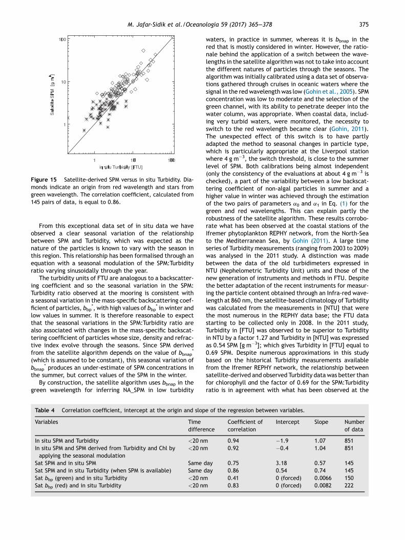
Figure 15 Satellite-derived SPM versus in situ Turbidity. Dia-monds indicate an origin from red wavelength and stars fromgreen wavelength. The correlation coefficient, calculated from145 pairs of data, is equal to 0.86.

M. Jafar-Sidik et al./Oceanologia 59 (2017) 365—378 375

From this exceptional data set of in situ data we haveobserved a clear seasonal variation of the relationshipbetween SPM and Turbidity, which was expected as thenature of the particles is known to vary with the season inthis region. This relationship has been formalised through anequation with a seasonal modulation of the SPM:Turbidityratio varying sinusoidally through the year.

The turbidity units of FTU are analogous to a backscatter-ing coefficient and so the seasonal variation in the SPM:Turbidity ratio observed at the mooring is consistent witha seasonal variation in the mass-specific backscattering coef-ficient of particles, bbp

*, with high values of bbp* in winter and

low values in summer. It is therefore reasonable to expectthat the seasonal variations in the SPM:Turbidity ratio arealso associated with changes in the mass-specific backscat-tering coefficient of particles whose size, density and refrac-tive index evolve through the seasons. Since SPM derivedfrom the satellite algorithm depends on the value of bbnap

*

(which is assumed to be constant), this seasonal variation ofbbnap

* produces an under-estimate of SPM concentrations inthe summer, but correct values of the SPM in the winter.

By construction, the satellite algorithm uses bbnap in thegreen wavelength for inferring NA_SPM in low turbidity

Table 4 Correlation coefficient, intercept at the origin and slop

Variables Timediffere

In situ SPM and Turbidity <20 nmIn situ SPM and SPM derived from Turbidity and Chl byapplying the seasonal modulation

<20 nm

Sat SPM and in situ SPM Same dSat SPM and in situ Turbidity (when SPM is available) Same dSat bbp (green) and in situ Turbidity <20 nmSat bbp (red) and in situ Turbidity <20 nm

waters, in practice in summer, whereas it is bbnap in thered that is mostly considered in winter. However, the ratio-nale behind the application of a switch between the wave-lengths in the satellite algorithm was not to take into accountthe different natures of particles through the seasons. Thealgorithm was initially calibrated using a data set of observa-tions gathered through cruises in oceanic waters where thesignal in the red wavelength was low (Gohin et al., 2005). SPMconcentration was low to moderate and the selection of thegreen channel, with its ability to penetrate deeper into thewater column, was appropriate. When coastal data, includ-ing very turbid waters, were monitored, the necessity toswitch to the red wavelength became clear (Gohin, 2011).The unexpected effect of this switch is to have partlyadapted the method to seasonal changes in particle type,which is particularly appropriate at the Liverpool stationwhere 4 g m�3, the switch threshold, is close to the summerlevel of SPM. Both calibrations being almost independent(only the consistency of the evaluations at about 4 g m�3 ischecked), a part of the variability between a low backscat-tering coefficient of non-algal particles in summer and ahigher value in winter was achieved through the estimationof the two pairs of parameters a0 and a1 in Eq. (1) for thegreen and red wavelengths. This can explain partly therobustness of the satellite algorithm. These results corrobo-rate what has been observed at the coastal stations of theIfremer phytoplankton REPHY network, from the North-Seato the Mediterranean Sea, by Gohin (2011). A large timeseries of Turbidity measurements (ranging from 2003 to 2009)was analysed in the 2011 study. A distinction was madebetween the data of the old turbidimeters expressed inNTU (Nephelometric Turbidity Unit) units and those of thenew generation of instruments and methods in FTU. Despitethe better adaptation of the recent instruments for measur-ing the particle content obtained through an Infra-red wave-length at 860 nm, the satellite-based climatology of Turbiditywas calculated from the measurements in [NTU] that werethe most numerous in the REPHY data base; the FTU datastarting to be collected only in 2008. In the 2011 study,Turbidity in [FTU] was observed to be superior to Turbidityin NTU by a factor 1.27 and Turbidity in [NTU] was expressedas 0.54 SPM [g m�3]; which gives Turbidity in [FTU] equal to0.69 SPM. Despite numerous approximations in this studybased on the historical Turbidity measurements availablefrom the Ifremer REPHY network, the relationship betweensatellite-derived and observed Turbidity data was better thanfor chlorophyll and the factor of 0.69 for the SPM:Turbidityratio is in agreement with what has been observed at the

e of the regression between variables.

nceCoefficient ofcorrelation

Intercept Slope Numberof data

0.94 �1.9 1.07 851 0.92 �0.4 1.04 851

ay 0.75 3.18 0.57 145ay 0.86 0.54 0.74 145

0.41 0 (forced) 0.0066 150 0.83 0 (forced) 0.0082 222

376 M. Jafar-Sidik et al./Oceanologia 59 (2017) 365—378

Liverpool Bay station. Focusing on Turbidity, and not non-algal SPM, Turbidity could be estimated directly from satel-lite-derived bbp by using the relationship shown in Fig. 13:

bbp½m�1� ¼ 0:0082 Turbidity ½FTU�:

4. Conclusion

At the location of the mooring in the Irish Sea, over an 8-yearperiod, we found results similar to those of Dogliotti et al.(2015) showing, at different coastal sites, that Turbidity is akey parameter to be estimated from marine reflectance. Thesemi-analytical methods in the red wavelength performrelatively well in low to medium Turbidity and Turbidity isretrieved with better success than SPM. The satellite-derivedbackscattering coefficient and the Turbidity are two opticalproperties that are tightly related. We have seen that apply-ing a seasonal modulation to the in situ Turbidity improvesthe estimation of SPM by diminishing the summer bias.Despite this clear seasonal variation of the particle typeand size that could affects the retrieving of SPM from satel-lite data processed by semi-analytical algorithms throughoutthe year, the switch operated in the satellite algorithm limitsthis effect at the location of the Liverpool Bay mooring. Asshown in Han et al. (2016) this algorithm provides relativelygood retrievals for a large variety of coastal waters whereSPM [g m�3] ranges within the limits [0,50]. We also knowthat in some places where the neap/spring cycle of Turbidityhas been observed from space (Shi et al., 2011; Rivier et al.,2012), the nature of the particles may change following thelunar cycle with bigger aggregates, therefore probably lowerbbnap

*, at neap tides. In other areas, like the continental shelfof the Bay of Biscay where the impact of the tidal cycle isrelatively low, a seasonal modification of the satellite algo-rithm could be proposed, with mass-specific backscatteringcoefficients in the green and the red different for the windywinter season and the summer (Gohin et al., 2015). bbnap

*

could be also determined partially from the intensity of thewaves, particularly in winter, whereas the spring to autumnvariability of bbnap

* induced by the biology could be improvedby a better knowledge of the TEPs (Transparent ExopolymerParticles). Improving our knowledge on the TEPs is a commonissue to remote-sensing and modelling of SPM (Van der Molenet al., 2009). The contribution of the phytoplankton to theIOPs and to the algal biomass could be also improved by usinglocal information on phytoplankton groups (observations oroutputs of ecological models). We can also mention the veryspecific signal of detached coccoliths, often visible on SPMimages in the North Atlantic, whose reflectance should beanalysed separately (Moore et al., 2012; Smyth et al., 2002).

In conclusion, Turbidity is probably the key parameter tobe estimated from space but as Turbidity measurements havebeen generally carried out in order to be transformed intoSPM using local calibrations, little attention has been paid tothe Turbidity values themselves and the variability of theturbidimeters is large in term of wavelengths and scatteringangles of observation. Remote-sensing is a good tool forhelping final users and turbidimeter builders to progress incooperation for defining instruments and calibration methodsbetter adapted to the monitoring of large coastal areas.

Acknowledgments

The authors are grateful to the Ocean Biology DistributedActive Archive Center at NASA, Greenbelt, MD, USA, for theprovision of MODIS-Aqua data. We are also grateful to theLiverpool Bay Coastal Observatory, National OceanographicCentre, UK for providing the SmartBuoy mooring data in theLiverpool Bay and NERC/DEFRA for funding the SmartBuoyand monitoring program. This work was carried out underMinistry of Higher Education (MOHE) Malaysia scholarshipwith collaboration with Universiti Malaysia Sabah (UMS). Italso contributes to the validation of the non-algal SPM pro-ducts provided for the Atlantic North-West Shelf by the OceanColour TAC of the Copernicus Marine Environment MonitoringService.

References

Berthon, J.F., Shybanov, E., Lee, M.E., Zibordi, G., 2007. Measure-ments and modeling of the volume scattering function in thecoastal northern Adriatic Sea. Appl. Opt. 46 (22), 5189—5203,http://dx.doi.org/10.1364/AO.46.005189.

Binding, C.E., Bowers, D.G., Mitchelson-Jacob, E.G., 2003. An algo-rithm for the retrieval of suspended sediment concentrations inthe Irish Sea from SeaWiFS ocean colour satellite imagery. Int. J.Remote Sens. 24 (19), 3791—3806, http://dx.doi.org/10.1080/0143116021000024131.

Bowers, D.G., Hill, P.S., Braithwaite, K.M., 2014. The effect ofparticulate organic content on the remote sensing of marinesuspended sediments. Remote Sens. Environ. 144, 172—178,http://dx.doi.org/10.1016/j.rse.2014.01.005.

Devlin, M.J., Barry, J., Mills, D.K., Gowen, J., Foden, J., Sivyer, D.,Greenwood, N., Pearce, D., Tett, P., 2009. Estimating the diffuseattenuation coefficient from optically active constituents in UKmarine waters. Estuar. Coast. Shelf Sci. 82 (1), 73—83, http://dx.doi.org/10.1016/j.ecss.2008.12.015.

Dogliotti, A.I., Ruddick, K.G., Nechad, B., Doxaran, D., Knaeps, E.,2015. A single algorithm to retrieve Turbidity from remotely senseddata in all coastal and estuarine waters. Remote Sens. Environ.156, 157—168, http://dx.doi.org/10.1016/j.rse.2014.09.020.

Edwards, K.P., Barciela, R., Butenschön, M., 2012. Validation of theNEMO-ERSEM operational ecosystem model for the North WestEuropean Continental Shelf. Ocean Sci. 8 (6), 983—1000, http://dx.doi.org/10.5194/os-8-983-2012.

Eleveld, M.A., Pasterkamp, R., Van der Woerd, H.J., Pietrzak, J.,2008. Remotely sensed seasonality in the spatial distribution ofsea-surface suspended particulate matter in the southern NorthSea. Estuar. Coast. Shelf Sci. 80 (1), 103—113, http://dx.doi.org/10.1016/j.ecss.2008.07.015.

Ford, D.A., van der Molen, J., Hyder, K., Bacon, J., Barciela, R.,Creach, V., McEwan, R., Ruardij, P., Forster, R., 2017. Observingand modelling phytoplankton community structure in the NorthSea. Biogeosciences 14 (6), 1419—1444, http://dx.doi.org/10.5194/bg-14-1419-2017.

Forget, P., Ouillon, S., Lahet, F., Broche, P., 1999. Inversion ofreflectance spectra of non-chlorophyllous turbid coastal waters.Remote Sens. Environ. 68 (3), 264—272, http://dx.doi.org/10.1016/S0034-4257(98)00117-5.

Gohin, F., 2011. Annual cycles of chlorophyll-a, non-algal suspendedparticulate matter, and Turbidity observed from space and in situin coastal waters. Ocean Sci. 7 (5), 705—732, http://dx.doi.org/10.5194/os-7-705-2011.

Gohin, F., Druon, J.N., Lampert, L., 2002. A five channel chlorophyllconcentration algorithm applied to SeaWiFS data processed by

M. Jafar-Sidik et al./Oceanologia 59 (2017) 365—378 377

Seadas in coastal waters. Int. J. Remote Sens. 23 (8), 1639—1661,http://dx.doi.org/10.1080/01431160110071879.

Gohin, F., Loyer, S., Lunven, M., Labry, C., Froidefond, J.M., Delmas, D.,Huret, M., Herbland, A., 2005. Satellite-derived parameters forbiological modeling in coastal waters: illustration over the easterncontinental shelf of the bay of Biscay. Remote Sens. Environ. 95 (1),29—46, http://dx.doi.org/10.1016/j.rse.2004.11.007.

Gohin, F., Bryère, P., Griffiths, J.W., 2015. The exceptional surfaceTurbidity of the North-West European shelf seas during the stormy2013—2014 winter: consequences for the initiation of the phyto-plankton blooms? J. Mar. Syst. 148, 70—85, http://dx.doi.org/10.1016/j.jmarsys.2015.02.001.

Guillou, N., Rivier, A., Gohin, F., Chapalain, G., 2015. Modeling near-surface suspended sediment concentration in the English chan-nel. J. Mar. Sci. Eng. 3 (2), 193—215, http://dx.doi.org/10.3390/jmse3020193.

Guillou, N., Rivier, A., Chapalain, G., Gohin, F., 2016. The impact oftides and waves on near-surface suspended sediment concentra-tions in the English Channel. Oceanologia 59 (1), 28—36, http://dx.doi.org/10.1016/j.oceano.2016.06.002.

Han, B., Loisel, H., Vantrepotte, V., Mériaux, X., Bryère, P.,Ouillon, S., Dessailly, D., Xing, Q., Zhu, J., 2016. Developmentof a semi-analytical algorithm for the retrieval of SuspendedParticulate Matter from remote sensing over clear to veryturbid waters. Remote Sens. 8 (3), 211, http://dx.doi.org/10.3390/rs8030211.

Huret, M., Gohin, F., Delmas, D., Lunven, M., Garcon, V., 2007.Use of SeaWiFS data for light availability and parameter esti-mation of a phytoplankton production model of the Bay ofBiscay. J. Mar. Syst. 65 (1—4), 509—531, http://dx.doi.org/10.1016/j.jmarsys.2005.07.007.

Lahet, F., Ouillon, S., Forget, P., 2000. A three-component model ofocean color and its application in the Ebro river mouth area.Remote Sens. Environ. 72 (2), 181—190, http://dx.doi.org/10.1016/S0034-4257(99)00101-7.

Li, Y., Huang, W., Fang, M., 1998. An algorithm for the retrieval ofsuspended sediment in coastal waters of China from AVHRR data.Cont. Shelf Res. 18 (5), 487—500, http://dx.doi.org/10.1016/S0278-4343(97)00074-5.

Loring, D.H., Rantala, R.T.T., 1992. Manual for the geochemicalanalyses of marine sediments and suspended particulate matter.Earth-Sci. Rev. 32 (4), 235—283, http://dx.doi.org/10.1016/0012-8252(92)90001-A.

Martinez-Vicente, V., Land, P.E., Tilstone, G.H., Widdicombe, C.,Fishwick, J.R., 2010. Particulate scattering and backscatteringrelated to water constituents and seasonal changes in the West-ern English Channel. J. Plankton Res. 32 (5), 603—619, http://dx.doi.org/10.1093/plankt/fbq013.

McKee, D., Cunningham, A., 2006. Identification and characterisa-tion of two optical water types in the Irish Sea from in situinherent optical properties and seawater constituents. Estuar.Coast. Shelf Sci. 68 (1—2), 305—316, http://dx.doi.org/10.1016/j.ecss.2006.02.010.

Ménésguen, A., Gohin, F., 2006. Observation and modelling of naturalretention structures in the English Channel. J. Mar. Syst. 63 (3—4),244—256, http://dx.doi.org/10.1016/j.jmarsys.2006.05.004.

Mills, D.K., Greenwood, N., Kröger, S., Devlin, M., Sivyer, D.B.,Pearce, D., Cutchey, S., Malcolm, S.J., 2005. New approachesto improve the detection of eutrophication in UK coastal waters.Environ. Res. Eng. Manage. 2 (32), 36—42.

Moore, T.S., Dowell, M.D., Franz, B.A., 2012. Detection of cocco-lithophore blooms in ocean color satellite imagery: a generalisedapproach for use with multiple sensors. Remote Sens. Environ.117, 249—263, http://dx.doi.org/10.1016/j.rse.2011.10.001.

Morel, A., 1988. Optical modelling of the upper ocean in relation to itsbiogeneous matter content (Case 1 water). J. Geophys. Res. 93 (C9),10749—10768, http://dx.doi.org/10.1029/JC093iC09p10749.

Nechad, B., Ruddick, K., Park, Y., 2010. Calibration and validation ofa generic multisensor algorithm for mapping of total suspendedmatter in turbid waters. Remote Sens. Environ. 114 (4), 854—866,http://dx.doi.org/10.1016/j.rse.2009.11.022.

Neil, C., Cunningham, A., McKee, D., 2011. Relationships betweensuspended mineral concentrations and red-waveband reflectancesin moderately turbid shelf seas. Remote Sens. Environ. 115 (12),3719—3730, http://dx.doi.org/10.1016/j.rse.2011.09.010.

Neukermans, G., Loisel, H., Mériaux, X., Astoreca, R., McKee, D.,2012. In situ variability of mass-specific beam attenuation andbackscattering of marine particles with respect to particle size,density, and composition. Limnol. Oceanogr. 57 (1), 124—144.

Reynolds, R.A., Stramski, D., Neukermans, G., 2016. Optical back-scattering by particles in Arctic seawater and relationships toparticle mass concentration, size distribution, and bulk composi-tion. Limnol. Oceanogr. 61 (5), 1869—1890, http://dx.doi.org/10.1002/lno.10341.

Rivier, A., Gohin, F., Bryère, P., Petus, C., Guillou, N., Chapalain, G.,2012. Observed vs. predicted variability in non-algal suspendedparticulate matter concentration in the English Channel in rela-tion to tides and waves. Geo-Mar. Lett. 32 (2), 139—151, http://dx.doi.org/10.1007/s00367-011-0271.

Sharples, J., Simpson, J.H., 1995. Semi-diurnal and longer periodstability cycles in the Liverpool Bay Region of Freshwater Influ-ence. Cont. Shelf Res. 15 (2—3), 295—313, http://dx.doi.org/10.1016/0278-4343(94)E0003-5.

Shi, W., Wang, M., Jiang, L., 2011. Spring-neap tidal effects onsatellite ocean color observations in the Bohai Sea, Yellow Sea,and East China Sea. J. Geophys. Res. Oceans 116 (C12), C12032,13 pp., http://dx.doi.org/10.1029/2011JC007234.

Smyth, T.J., Moore, G.F., Groom, S.B., Land, P.E., Tyrrell, T., 2002.Optical modeling and measurements of a coccolithophore bloom.Appl. Opt. 41 (36), 7679—7688, http://dx.doi.org/10.1364/ao.41.007679.

Snyder, W.A., Arnone, R.A., Davis, C.O., Goode, W., Gould, R.W.,Ladner, S., Lamela, G., Rhea, W.J., Stavn, R., Sydor, M., Weide-mann, A., 2008. Optical scattering and backscattering by organicand inorganic particulates in U.S. coastal waters. Appl. Opt. 47(5), 666—677, http://dx.doi.org/10.1364/AO.47.000666.

Sykes, P.A., Barciela, R.M., 2012. Assessment and development ofa sediment model within an operational system. J. Geophys.Res. 117 (C4), C04036, 17 pp., http://dx.doi.org/10.1029/2011JC007420.

Tett, P.B., 1987. Plankton. In: Baker, J.M., Wolff, W.J. (Eds.), Bio-logical Surveys of Estuaries and Coasts. Cambridge Univ. Press,Cambridge, 280—341.

Tilstone, G., Mallor-Hoya, S., Gohin, F., Belo Couto, A., Sa, C., Goela,P., Cristina, S., Airs, R., Icely, J., Zühlke, M., Groom, S., 2017.Which Ocean colour algorithm for MERIS in North West Europeanwaters? Remote Sens. Environ. 189, 132—151, http://dx.doi.org/10.1016/j.rse.2016.11.012.

Van der Molen, J., Bolding, K., Greenwood, N., Mills, D.K., 2009. A 1-D vertical multiple grain size model of suspended particulatematter in combined currents and waves in shelf seas. J. Geophys.Res. 114 (F1), F01030, 15 pp., http://dx.doi.org/10.1029/2008JF001150.

Van der Molen, J., Ruardij, P., Greenwood, N., 2016. Potentialenvironmental impact of tidal energy extraction in the PentlandFirth at large spatial scales: results of a biogeochemical model.Biogeosciences 13 (8), 2593—2609, http://dx.doi.org/10.5194/bg-13-2593-2016.

378 M. Jafar-Sidik et al./Oceanologia 59 (2017) 365—378

Van der Molen, J., Ruardij, P., Greenwood, N., 2017. A 3D SPM modelfor biogeochemical modelling, with application to the northwestEuropean continental shelf. J. Sea Res., http://dx.doi.org/10.1016/j.seares.2016.12.003 (in press).

Van der Woerd, H.J., Pasterkamp, R., 2008. HYDROPT: a fast andflexible method to retrieve chlorophyll-a from multispectralsatellite observations of optically complex coastal waters. Re-mote Sens. Environ. 112 (4), 1795—1807, http://dx.doi.org/10.1016/j.rse.2007.09.001.

Wolf, J., Brown, J.M., Howarth, M.J., 2011. The wave climate ofLiverpool Bay — observations and modelling. Ocean Dynam. 61(5), 639—655, http://dx.doi.org/10.1007/s10236-011-0376-9.

Woźniak, S.B., 2014. Simple statistical formulas for estimating bio-geochemical properties of suspended particulate matter in thesouthern Baltic Sea potentially useful for optical remote sensingapplications. Oceanologia 56 (1), 7—39, http://dx.doi.org/10.5697/oc.56-1.007.