raf - universiti teknikal malaysia melaka...

A-raf

0000099281 TNB load reading prediction I Muhamad Najmi Abu Bakar.

I

] .

TNB LOAD READING PREDICTION

Muhamad Najmi bin Abu Bakar

Bachelor of Power Electronics and Drive

June 2012

© Universiti Teknikal Malaysia Melaka

A STUDY ON

TNB LOAD READING PREDICTION

MUHAMAD NAJMI BIN ABU BAKAR

This Report Is Submitted In Partial Fulfillment of Requirement for the Degree of

Bachelor in Electrical Engineering (Power Electronic and Drives)

Faculty of Electrical .Engineering

UNIVERSITI TEKNIKAL MALAYSIA MELAKA

JUNE2012


l

I

J

"I hereby declared that I have read through this report entitle " A Study On TNB Load

Reading Prediction" and found that it has comply the partial fulfillment for awarding the

degree ofBachelor of Electrical Engineering (Power Electronic and Drives)"

Signature

Supervisor's Name

Date

ENCIK NORAZHAR BIN ABU BAKAR

.... ...... :f-:5"/?./ ~ 1~ .. ............ · ........................ .


l

J

I

I I

j

"I hereby declared that this report is of my own work except for the excerpts that have

been cited clearly in the references "

Signature .. fo ... . ......... . Name MUHAMAD NAJMI BIN ABU BAKAR

Date 2s (G I ~o\2


I

I

I

I 1

J

Dedicated to my beloved Parents, my siblings

Lectures and all my friends

For their love and sacrifice.


I

I

. I

11

ACKNOWLEDGEMENT

In the name of Allah S.W.T, the most gracious and merciful, praise to Allah the

lord of universe and may blessing and peace of Allah be upon his messenger Muhammad

S.A.W. First, and foremost thank to Allah for giving me wellness and ideas to complete

this project report. Without any of it, I smely cannot complete this project in the time

given.

I would like to express my appreciation to my project supervisor, En .. Norazhar bin

Abu Bakar for giving brilliant advices and guidance to me as well as provision of the

valuable time management, encouragement and patience during the time period of

completing this project.

Last but not least, I like to express my very thankful and send our grateful to my

entire friend and my family for the moral and fmancial support. To those that I forget to

mention, please forgive me. I do appreciate all the things you have done for me .


l 1

{

t

J

t

111

ABSTRACT

Nowadays there is a growing tendency towards improving the electricity system. Load

forecasting is a process of predicting the future load demands. The growth of development

in the country increases the demand on planning management and operations of the power

system supply. As electricity is a product that cannot be stored, it demands must be

· forecasted in order to ensure enough supply being di$tributed to_ consumers while not

generating load far exceeded that required. This project paper demonstrates the

development of forecasting modeling by the application of Matlab software. It covers the

load demand by the users in Penang. Hence, the load data from TNB has been used as

input to forecast load and the temperature data from Malaysia ·Meteorology Department

also had been used as forecasting factors. The forecasted load had been compared with

actual load data to get the minimum forecasting error and better accuracy. The neural

network modeling is able to make a prediction of what load would be in the next day. The

modeling showed that neural network was used widely and accurately in load forecasting.


J

J

IV

ABSTRAK

Sejak kebelakangan ini berlaku peningkatan ke arab. penambahbaikan sistem elektrik.

Ramalan beban adalah satu proses meramal permintaan tenaga elektrik di masa hadapan.

Pertumbuban pembangunan di negara ini meningkatkan lagi keperluan kepada pengurusan

perancangan serta operasi sistem bekalan kuasa. Tenaga elektrik adalah produk yang tidak

boleh disimpan, ia harus dianggarkan dalam usaha untuk memastikan bekalan yang

mencukupi untuk dibekalkan kepada pengguna di samping tidak menjana tenaga elektrik

yang jauh melebihi keperluan. Projek ini menghasilkan pembangunan model ramalan

meggunakan aplikasi perisian Matlab. Ia meliputi permintaan tenaga elektrik oleh

pengguna di Pulau Pinang. Oleh itu, data tenaga elektrik daripada TNB telah digunakan

sebagai input untuk meramalkan tenaga dan data suhu daripada Jabatan Meteorologi

Malaysia juga telah digunakan sebagai faktor ramalan. Beban ramalan telah dibandingkan

dengan data beban sebenar untuk mendapatkan ralat ramalan minimum dan ketepatan yang

lebih baik. Permodelan ini mampu untuk membuat ramalan beban yang akan digunakan di

hari berikutnya. Permodelan menunjukkan bahawa rangkaian ini telah digunakan secara

meluas dan tepat dalam ramalan beban.


3

-4

2.5

2.4.3.6 Multi Layered Neural Network

2.4.3.7 Hidden Layer and Node

2.4.3.8 Hidden Neuron

2.4.3.9 Learning Rate

2.4.3.10Momentum Rate

Study the Related Journal

METHODOLOGY

3.1 Overview of Methodology

3.1.1 Do the research about the topic

(LiteratUre Review)

3.1.2 Data Gathering

3.1.3 Develop modeling in Matlab (Training)

3 .1.3 .1 Using Matlab 7 .12. 0 software

3.1.3.2 Assemble Training Data

3.1.3.3 Create Network or Data

3.1.3.4 Train Network

3.1.3.5 Simulation Process

3.1.3.6 Get Result Forecast

RESULT

4.1 Forecast Results of Power Consumption for Every

Month

4.1.1 Forecasting Results for January

4.1.2 Forecasting Results for February

4.1.3 Forecasting Results for March

4.1.4 Forecasting Results for April

4.1.5 Fore casting Results for May

4.1.6 Forecasting Results for June

4.1.7 Forecasting Results for July

4.1.8 Forecasting Results for August

4.1.9 Forecasting Results for September

. © Universiti Teknikal Malaysia Melaka

10

10-11

11

11

12

12-15

16

16-17

18

18

18-19

20

2 1- 22

23 - 24

24-28

29

30

31

31

31 - 33

33 - 34

34 - 36

36-37

38-39

39 --, 40 .

41 - 42

42-43

44 - 45

Vl

5

6

4 .1.1 0 Forecasting Results for October

4.1.11 Forecasting Results for November

4.1.12 Forecasting Results for December

ANALYSIS & DISCUSSION OF RESULT

5.1 Analysis for January Load Forecast

5.2 Analysis for February Load Forecast

5.3 Analysis for March Load Forecast

5.4 Analysis for April Load Forecast

5.5 Analysis for May Load Forecast

5.6 Analysis for June Load Forecast

5.7 Analysis for July Load Forecast

5.8 Analysis for August Load Forecast

5.9 Analysis for September Load Forecast

5.10 Analysis for October Load Forecast

5.11 Analysis for November Load Forecast

5.12 Analysis for December Load Forecast

5.13 The Mean Absolute Percentage Error for Each Month

SUMMARY AND CONCLUSION

6.1

6.2

6.3

Summary

Conclusion

Recommendation

REFERENCES

APPENDIX


45 - 47

47-48

48-49

50

50-51

51-52

52 -53

53-54

55

56- 57

57-58

58-59

59

60 - 61

61-62

62-63

63-64

65

65

66-67

67

68-69

70

vii

viii

LIST OF TABLES

TABLE TITLE PAGE

4.1 Forecasting Results for January 31-32

4.2 Forecasting Results for February 33-34

4.3 Forecasting Results for March 35

4.4 Forecasting Results for April 36-37

4.5 Forecasting Results for May 38

4.6 Forecasting Results for June 39-40

4.7 Forecasting Results for July 41

4.8 Forecasting Results for August 42--43

4.9 Forecasting Results for September 44

4.10 Forecasting Results for October 45-46

4.11 Forecasting Results for November 47

4.12 Forecasting Results for December 48-49

5.1 Percentage Error for February 52

5.2 Percentage Error for March 53

5.3 Percentage Error for April 54

5.4 Percentage Error for June 56-57

5.5 .Percentage Error for July 58

5.6 Percentage Error for October 60

5.7 Percentage Error for November 62

5 .8 The Mean Absolute Percentage Error for Each Month 63


lX

LIST OF FIGURES

NO TITLE PAGE

2.1 The model of neuron in hidden layer 8

2.2 None linear model of neuron 8

2.3 The types of transfer function 9

2.4 Single layered neural network 10

2.5 Multilayered neural network 10

2.6 A Generalized Network 14

2.7 The Structure of a Neuron 14

3.1 Flow Chart of Overall Methodology 17

3.2 Flow Chart of Develop Neural Network model in Matlab 19

3.3 Neural Network tool window 20

3.4 Neural Network tool window 20

3.5 Input and target data arranged 21

3.6 Input data created 21

3.7 Target data created 22

3.8 Netw·ork/data manager 22

3.9 Network or data Window 23

3.10 View ofNew Network 1 (2layers) 24

.3.11 Training info of the network 25

3.12 Training parameters of the network .25

3.13 Neural network training (nntraintool) 26

3.14 Performance (plot perform) 27

3.15 Regression (plot regression) 28

3.16 Simulate the network 29

3.17 Data, network output (forecast result) 29

3.18 Network output (forecast result) 30

4.1 January Load Forecast 32

4.2 February Load Forecast 34

4 .3 March Load Forecast 36


X

4.4 April Load Forecast 37

4.5 May Load Forecast 38

4.6 June Load Forecast 40

4.7 July Load Forecast 42

4.8 August Load Forecast 43

4.9 September Load Forecast 45

4.10 October Load Forecast 46

4.11 November Load Forecast 48

4.12 December Load Forecast 49

5.1 Comparison Load Pattern on January 50

5.2 Comparison Load Pattern on February 51

5.3 Comparison Load Pattern on March 52

5.4 Comparison Load Pattern on April 53

5.5 Comparison Load Pattern on May 55

5.6 Comparison Load Pattern on June 56

5.7 Comparison Load Pattern on July 57

5.8 Comparison Load Pattern on August 58

5.9 Comparison Load Pattern on September 59

5.10 Comparison Load Pattern on October 60

5.11 Comparison Load Pattern on November 61

5.12 Comparison Load Pattern on December 62

5.13 Mean Percentage Absolute Error (MAPE) 64


LIST OF APPENDIX

NO TITLE

A Project Planning


PAGE

70

Xl

CHAPTER!

INTRODUCTION

1.0 Background

Tenaga Nasional Berhad (TNB) is the largest of electricity utility company in

Malaysia. Their core activities are in the generation, transmission and distribution of

electricity. These activities ranging from system planning, evaluating, implementing and

maintaining the systems. One of the requirements of the system planning is load

forecasting. Load forecasting is a prediction of power demand. It is important for

electricity planning and to ensuring that there would be enough supply of electricity, where

and when that power must delivered. The accurate forecasting of energy requirement is one

of the most important factors of energy management for the future development of the

country like Malaysia. It can give a better planning such as budget planning, maintenance

scheduling, the reliability evaluation of the power system and many more. Many factors

are related to load forecasting such as weather changes, temperature, season, population,

number of electricity consumers and others. Load forecast also can divides in three

catogeries that is Long Term Load Forecast (LTLF), Medium Term Load Forecast (MTLF)

and Short Term Load Forecast (STLF).

1.1 Problem Statements

Load forecasting is an important component in the operation and planning of

electrical power generation conducted by Utilities Company. Many factors can influence

the electricity usage. One of the factors is temperature changes and it made difficultly for

TNB to predict power demand. It can affected the budget planning, maintenance and also

electricity blackout. In order to overcol?e this problem a predicting model can be used


2

based on history and forecast data. These data were analyzed to give better accuracy for

future load demand. The electric utility company should have an appropriate model for

load forecasting to ensure balance need among the utility and environment factors as well

as minimizing the operating cost. For this project, an algoritlun modeling will be

developed to predict power demand based on temperature condition. A neural networks

methods have been used to developed load forecasting modeling by using Matlab software.

Hopefully this project will give some benefits to the utility of Malaysia in order to improve

load forecasting in Malaysia.

1.2 Objectives

1.2.1 To develop an algorithm model to predict power demand based on temperature

condition in Malaysia.

1.2.2 To investigate performance and accuracy of power demand prediction based on

temperature condition.

1.3 Scopes of The Project

The project will focusing on developing an algorithm by using MATLAB software.

It will be used to simulate and analyze forecasting load data. The result between forecasted

load and actual load data will be compared to fmd forecasting error. The variables

considered in this project are based on power demand and temperature changes data.The

focusing area for this project is in Penang, so that the load demand data from TNB has

been taken this area by a year which is from January to December 2011. The temperature

data for this area also has been taken from Malaysia Meteorology Department.


CHAPTER2

LITERATURE REVIEW

Load forecasting is very important to use in the system and market operators,

transmission owners and any other market participants. It also can help an electric utility

company such as Tenaga Nasional Berhad (TNB) to make decisions including on

purchasing and generating electric power, load switching and infrastructure growth.

Forecasting also can be divide into three categories that each category has a different time

ranges. This is an important task to utility company for achieving the goal of optimal

planning and operation of power system. The categories are Long Term Load Forecasting

(LTLF), Mediwn Term Load Forecasting (MTLF) and Short Term Load Forecasting

(STLF). Each category has a forecast method to development more accurate load

forecasting.

2.1 Long Term Load Forecasting (LTLF)

The estimation may lead utility company to plan the generation and distribution

schedule. It had been done for various lead times ranging from few seconds to more than a

year. Long term load forecasting is an important issue in effective and efficient planning.

Overestimation of power demand may lead to spending more money in building new

power stations to supply this load. However, underestimation of load can cause troubles in

supplying load from the available electric supplies, and produce a shortage in spinning

reserve of the system that may lead to an insecure and defective system [2]. Long term

load forecasting is the forecasting of future loads for a relatively large lead time (years

ahead). It includes the forecasts on the population changes, economic development,

industrial construction and technology development (1]. In fact, there have a few published

paper can be found on the long term situation. The reason of this case because the long

term forecasting requires years of econo!llic and demographic data which may not be easy


4

to gather or access. Even when data is accessible, it was complexes in the sense that it is

affected by environmental, economical, political and social factors [2].

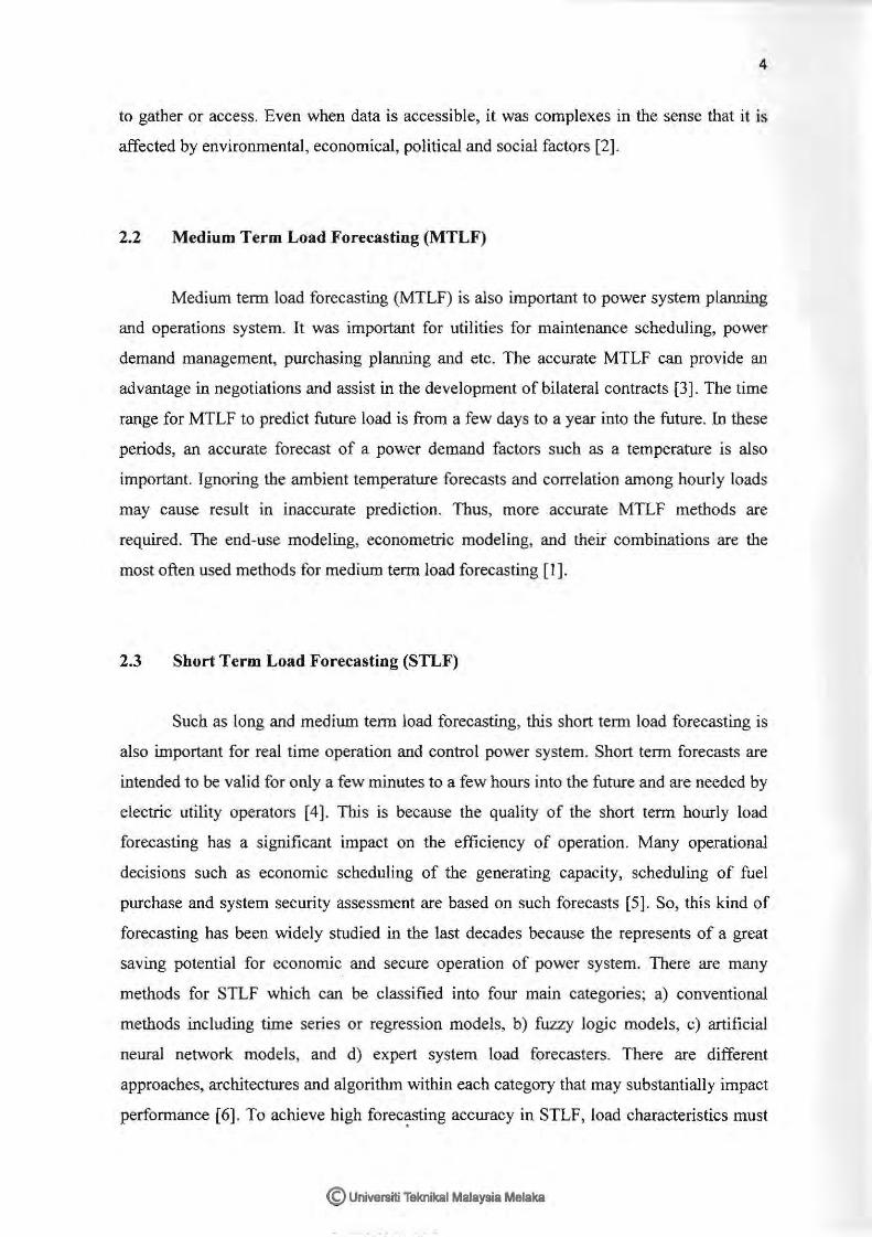
2.2 Medium Term Load Forecasting (MTLF)

Medium term load forecasting (MTLF) is also important to power system planning

and operations system. It was important for utilities for maintenance scheduling, power

demand management, purchasing planning and etc. The accurate MTLF can provide an

advantage in negotiations and assist in the development of bilateral contracts [3]. The time

range for MTLF to predict future load is from a few days to a year into the future. In these

periods, an accurate forecast of a power demand factors such as a temperature is also

important. Ignoring the ambient temperature forecasts and correlation among hourly loads

may cause result in inaccurate prediction. Thus, more accurate MTLF methods are

required. The end-use modeling, econometric modeling, and theii combinations are the

most often used methods for medium term load forecasting [ 1].

2.3 Short Term Load Forecasting (STLF)

Such as long and medium term load forecasting, this short term load forecasting is

also important for real time operation and control power system. Short term forecasts are

intended to be valid for only a few minutes to a few hours into the future and are needed by

electric utility operators [4]. This is because the quality of the short term hourly load

forecasting has a significant impact on the efficiency of operation. Many operational

decisions such as economic scheduling of the generating capacity, scheduling of fuel

purchase and system security assessment are based on such forecasts [5]. So, this kind of

forecasting has been widely studied in the last decades because the represents of a great

saving potential for economic and secure operation of power system. There are many

methods for STLF which can be classified into four main categories~ a) conventional

methods including time series or regression models, b) fuzzy logic models, c) artificial

neural network models, and d) expert system load forecasters. There are different

approaches, architectures and algorithm within each category that may substantially impact

performance [6]. To achieve high forec~sting accuracy in STLF, load characteristics must


5

be analyzed therefore the main factors affecting the load can be identified. Some factors of

influencing the load that need to be considered in STLF are season, day type, weather and

electric price [1].

2.4 Forecasting Methods

There are many methods can be used in forecasting such as time series method,

fuzzy logic method, neural network method, regression method and others else. For this

project, Neural Network method will be applied in order to give a faster and accurate result

compared with other conventional method like Statistical, time series, perceptron. Matlab

software is used to develop this neural network model.

2.4.1 Neural Network

Neural networks, or artificial neural networks (ANN) as they are often called, refer

to a class of models inspired by biological nervous systems. The models are composed of

many computing elements, usually denoted neurons, working in parallel. The elements are

connected by synaptic weights, which are allowed to adapt through a learning process.

There are many types of neural network models, the common feature in them being

the connection of the ideas to biological systems. The models can be categorized in many

ways. One possibility is to classify them on the basis of the learning principle. A neural

network uses either supervised or unsupervised learning. In supervised learning, the

network is provided with example cases and desired responses. The network weights are

then adapted in order to minimize the difference between network outputs and desired

outputs. In unsupervised learning the network is given only input signals, and the network

weights change through a predefined mechanism, which usually groups the data into

clusters of similar data. The most common network type using supervised learning is a

feed-forward (signal transfer) network. The network is given an input signal, which is

transferred forward through the network. Eventually, an output signal is produced. The

network can be understood as a mapping from the input space to the output space, and this


6

mapping is defmed by the free parameters of the model, which are the synaptic weights

connecting the neurons [7,8].

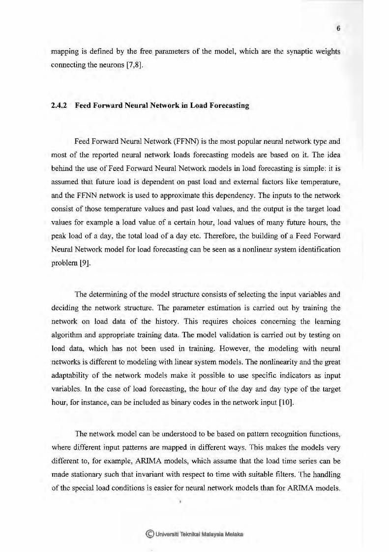
2.4.2 Feed Forward Neural Network in Load Forecasting

Feed Forward Neural Network (FFNN) is the most popular neural network type and

most of the reported neural network loads forecasting models are based on it. The idea

behind the use of Feed Forward Neural Network models in load forecasting is simple: it is

assumed that future load is dependent on past load and external factors like temperature,

and the FFNN network is used to approximate this dependency. The inputs to the network

consist of those temperature values and past load values, and the output is the target load

values for example a load value of a certain hour, load values of many future hours, the

peak load of a day, the total load of a day etc. Therefore, the building of a Feed Forward

Neural Network model for load forecasting can be seen as a nonlinear system identification

problem [9].

The determining of the model structure consists of selecting the input variables and

deciding the network structure. The parameter estimation is carried out by training the

network on load data of the history. This requires choices concerning the learning

algorithm and appropriate training data. The model validation is carried out by testing on

load data, which has not been used in training. However, the modeling with neural

networks is different to modeling with linear system models. The nonlinearity and the great

adaptability of the network models make it possible to use specific indicators as input

variables. In the case of load forecasting, the hour of the day and day type of the target

hour, for instance, can be included as binary codes in the network input [1 0].

The network model can be understood to be based on pattern recognition functions,

where different input patterns are mapped in different ways. This makes the models very

different to, for example, ARIMA models, which assume that the load time series can be

made stationary such that invariant with respect to time with suitable filters. The handling

of the special load conditions is easier for neural network models than for ARIMA models.


7

Another matter supporting neural network models is the relatively rapid changing of the

characteristics in the load behavior. This is a problem with statistical models, because they

cannot always keep up with the sudden changes in the dependencies of the load. For

example, the beginnings of holiday seasons etc. can change the load behavior rapidly. As

neural network models are in essence based on pattern recognition functions, they can in

principle be hoped to recognize the changed conditions without re-estimating the

parameters. This requires of course that conditions corresponding to the new situation have

been used in training, and that network inputs contain the information necessary for

recognizing the conditions. On the other hand, a problem with Feed Forward Neural

Network models is the black-box like description of the dependencies of the future values

on the past behavior. The understanding of the model is very difficult; the common sense

can hardly be applied in order to see how the outputs depend on inputs. The responding of

the model to an input pattern, which is very different to any experienced during the

learning, can be unexpected. This can happen in new conditions, even if the model is

validated with test data [ 11].

2.4.3 Component of Neural Network

2.4.3.1 Input and Output Factor

Selection of input is the most important part that has an impact on

the desired output. Neurons in the input layer are not neurons in processing

elements (PEs) sense; they act as simple fan out devices which passes the

input to the various neurons in the next (hidden) layer without doing any

processing. Therefore, the number of input layer neurons is fl.Xed by the

number of scalars in the input vector. As each neuron provides only a single

output, the number of neurons required in the output layer will be equal to

the number of scalars in the output vector. Improper selection of input will

cause divergence, longer learning time and inaccuracy reading that is

greater than 1.


2.4.3.2

2.4.3.3

8

Weighting factor

Relative weighting will be installing in each input and this weighting

will affected the impact the input as shown in Figure 2.1. Weights

determine the intensity of the input signal and are adaptive coefficients

within the network. To various input, the initial weight for PE can be

modified and according to the network's own rules for modification.

Figure 2.1: The model of neuron in hidden layer [6]

Neuron model

Fundamental processing element of a neural network is a neuron.

The network usually consists of an input layer, some hidden layers and an

output layer. The model of a neuron is shown in Figure 2.2

\I

\.

'> l li. II <LII. \ la.l('l_!..!lll ...

r. • J

n u,•,h .. IJ

Figure 2.2 : non linear model of neuron [ 12]


2.4.3.4

9

Transfer function

There are a lot of transfer functions and basically the transfer

function is a non-linear. A non-linear system is a system which is not linear,

that is a system which does not satisfy the superposition principle, or whose

output is notdirectly proportional to its input. The linear also known a

straight line and the linear function is limited because the output is

proportional to the input. Although, the output is depends upon whether the

result of summation is negative or positive. The network output can be 1

and -1, or 1 and 0.

The hard limiter transfer function was used in perceptrons to create neurons

that make classification decisions. For the linear transfer function, neurons

of this type are used as linear approximates in linear filters. The sigmoid

transfer function takes the input which can have any value between positive

and negative infinity, and squashes the output into the range 0 to 1. Figure

2.3 show the type of transfer function.

a a

+l

----f--0 ~II []

-l

(a) (b)

-l

(c)

Figure 2.3: The types of transfer function. (a) Hard limiter (b) Linear function

(c) Sigmoid function (12]

2.4.3.5 Single layer neural network

A single or one layer neural network do not have hidden layer and it

is characterized by a layer of input neurons and a layer of output neurons

interconnected to one another by weight to be determined in training

process. This single layer neural network cannot give an accurate result in


2.4.3.6

2.4.3.7

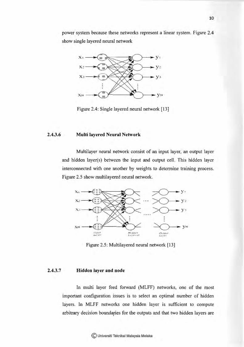
10

power system because these networks represent a linear system. Figure 2.4

show single layered neural network

Figure 2.4: Single layered neural network [13]

Multi layered Neural Network

Multilayer neural network consist of an input layer, an output layer

and hidden layer(s) between the input and output cell. This hidden layer

interconnected with one another by weights to determine training process.

Figure 2.5 show multilayered neural network.

!•lJ;'id L,..l , .:r

• ...-fi ... .. <t:T, .:..... ... t"C'' • • •

~YN

Figure 2.5: Multilayered neural network [13]

Hidden layer and node

In multi layer feed forward (MLFF) networks, one of the most

important configuration issues is to select an optimal number of hidden

layers. In MLFF networks one hidden layer is sufficient to compute

arbitrary decision boundapes for the outputs and that two hidden layers are


raf - universiti teknikal malaysia melaka...

Documents