apportitecnici

GPU implementation and validation offully three-dimensional multi-fluidSPH models

Anno 2014_Numero 292

Istituto Nazionale di

Geofisica e Vulcanologia

tISSN 2039-7941

t

Direttore ResponsabileStefano Gresta

Editorial BoardAndrea Tertulliani - Editor in Chief (INGV - RM1)Luigi Cucci (INGV - RM1)Nicola Pagliuca (INGV - RM1)Umberto Sciacca (INGV - RM2)Alessandro Settimi (INGV - RM2)Aldo Winkler (INGV - RM2)Salvatore Stramondo (INGV - CNT)Milena Moretti (INGV - CNT)Gaetano Zonno (INGV - MI)Viviana Castelli (INGV - BO)Antonio Guarnieri (INGV - BO)Mario Castellano (INGV - NA)Mauro Di Vito (INGV - NA)Raffaele Azzaro (INGV - CT)Rosa Anna Corsaro (INGV - CT)Mario Mattia (INGV - CT)Marcello Liotta (Seconda Università di Napoli, INGV - PA)

Segreteria di RedazioneFrancesca Di Stefano - ReferenteRossella CeliBarbara AngioniTel. +39 06 51860068Fax +39 06 36915617

redazionecen@ingv.it

REGISTRAZIONE AL TRIBUNALE DI ROMA N.173|2014, 23 LUGLIO© 2014 INGV Istituto Nazionale di Geofisica e VulcanologiaSede legale: Via di Vigna Murata, 605 | Roma

GPU IMPLEMENTATION AND VALIDATION OF FULLY THREE-DIMENSIONAL MULTI-FLUID SPH MODELS

Giuseppe Bilotta

INGV (Istituto Nazionale di Geofisica e Vulcanologia, Sezione di Catania - Osservatorio Etneo)

Anno 2014_Numero 292t

apportitecnici

ISSN 2039-7941

Table of contents

Introduction ........................................................................................................................................................ 7  

1.   Single-fluid weakly-compressible SPH for fluid dynamics ........................................................................ 7  

1.1.   Classic SPH for fluid dynamics ............................................................................................................... 7  

1.1.1.   Standard SPH interpolation for fields ................................................................................................... 7  

1.1.2.   SPH for first derivatives ...................................................................................................................... 10  

1.1.3.   SPH for second derivatives ................................................................................................................. 11  

1.2.   Navier-Stokes equations and their SPH discretization ........................................................................... 11  

1.3.   Speed of sound in SPH ........................................................................................................................... 13  

2.   SPH and parallel computing: GPUSPH .................................................................................................... 13  

2.1.   GPUSPH structure .................................................................................................................................. 14  

2.1.1.   Integration scheme .............................................................................................................................. 14  

2.1.2.   The neighbor list .................................................................................................................................. 15  

2.1.3.   Boundary conditions ........................................................................................................................... 15  

3.   Multi-fluid SPH models ............................................................................................................................ 16  

3.1.   Introduction ............................................................................................................................................ 16  

3.2.   Hu & Adams multi-fluid model ............................................................................................................. 16  

3.2.1.   Formulation ......................................................................................................................................... 16  

3.2.2.   Boundary conditions and ghost particles ............................................................................................ 17  

3.2.3.   Implementation notes .......................................................................................................................... 18  

3.3.   Grenier’s multi-fluid model ................................................................................................................... 19  

3.3.1.   Formulation ......................................................................................................................................... 19  

3.3.2.   Boundary conditions and surface tension ............................................................................................ 20  

3.3.3.   Implementation notes .......................................................................................................................... 21  

4.   Validation .................................................................................................................................................. 22  

4.1.   Introduction ............................................................................................................................................ 22  

4.1.1.   Description of the test cases ................................................................................................................ 22  

4.2.   Smoothing kernels .................................................................................................................................. 22  

4.3.   Rayleigh-Taylor instability .................................................................................................................... 23  

4.3.1.   Hu & Adams’ formulation .................................................................................................................. 24  

4.3.2.   Grenier’s formulation .......................................................................................................................... 25  

4.3.3.   Validation ............................................................................................................................................ 27  

4.3.4.   Numerical precision ............................................................................................................................ 28  

4.4.   Lock exchange / Gravity current ............................................................................................................ 30  

4.4.1.   Influence of formulation and surface tension ...................................................................................... 30  

4.4.2.   Influence of resolution ........................................................................................................................ 34  

4.5.   Rising bubble .......................................................................................................................................... 35  

4.5.1.   Two-dimensional problem .................................................................................................................. 35  

4.5.2.   Influence of surface tension ................................................................................................................ 37  

4.5.3.   Three-dimensional problem ................................................................................................................ 38  

5.   Conclusions and prospective for future work ........................................................................................... 40  

5.1.   Conclusions ............................................................................................................................................ 40  

5.2.   Prospective for future work .................................................................................................................... 41  

Acknowledgements .......................................................................................................................................... 41  

References ........................................................................................................................................................ 41  

7

Introduction Computational fluid dynamics (CFD) provides the mathematical and computational tools for the

numerical simulations of fluid flows, an essential component in a number of applications ranging from geophysics to industrial applications. It can be used to forecast the areas subject to potential inundation by natural flows (tsunamis, lava flows, landslides, pyroclastic flows), to evaluate the impact and cost of strategies aimed at reducing long- and short-term risk from natural and man-made hazards, or to test mechanical designs and verify their efficiency before the costly implementation processes.

In many applications, multiple fluids (e.g. oil, water, air) may be present in the same problem, and the very different rheological properties of these fluids pose a challenge for some CFD methods. The work described in this report is focused on the implementation and validation of two state-of-the-art multi-fluid models for the Smoothed Particles Hydrodynamics (SPH) numerical method.

The SPH method, in its weakly-compressible formulation, is highly parallelizable, and is therefore an excellent candidate for impementation on parallel computing hardware, such as Graphic Processing Units (GPUs). While GPUs have been primarily developed for high-performance three-dimensional graphic rendering and video-games, since 2007 the two major manufacturers have also exposed their massive parallel computing capabilities to more generic applications. Our work is integrated into GPUSPH [Hérault et al., 2010], the first implementation of SPH to use CUDA-enabled GPUs as high-performance parallel computing devices.

The report begins with an introduction to the SPH method and its application to the Navier-Stokes equations for fluid dynamics, highlighting the issues that the classical SPH formulation encounters in the case of multiple fluids. This is followed by an overview of GPUSPH, the implementation of SPH on CUDA GPUs which is the basis for our implementation of the multi-fluid SPH models: the Hu & Adams model [Hu and Adams, 2006], and the more recent one developed by Grenier [Grenier et al., 2008; 2009; Grenier, 2009]. A description of these models, highlighting the differences over the classic SPH formulation, is included in the subsequent chapter. Finally, validation tests are shown for problems in both two and three dimensions, covering the classic Rayleigh-Taylor instability, the lock exchange gravity current problem, and finally a rising bubble example.

To the best of our knowledge, the work described here represent the first fully three-dimensional implementation of these multi-fluid SPH models on the high-performance computing platform provided by CUDA-enabled GPUs.

1. Single-fluid weakly-compressible SPH for fluid dynamics

1.1. Classic SPH for fluid dynamics Smoothed Particles Hydrodynamics (SPH) is a meshless Lagrangian method, where the fluid is

discretized using virtual interpolation nodes (particles) that are not fixed in any predefined mesh and whose evolution is described by the equation of motion of the fluid itself. Among the advantages of SPH we have the direct computation of all required physical quantities and their gradients, the implicit tracking of surfaces (such as the free surface of the flow or internal solidification fronts in the case of thermal evolutions with phase transition), as well as the ability to cope with large deformations without any need for remeshing (which is typically needed e.g. with the Finite Elements Method).

1.1.1. Standard SPH interpolation for fields

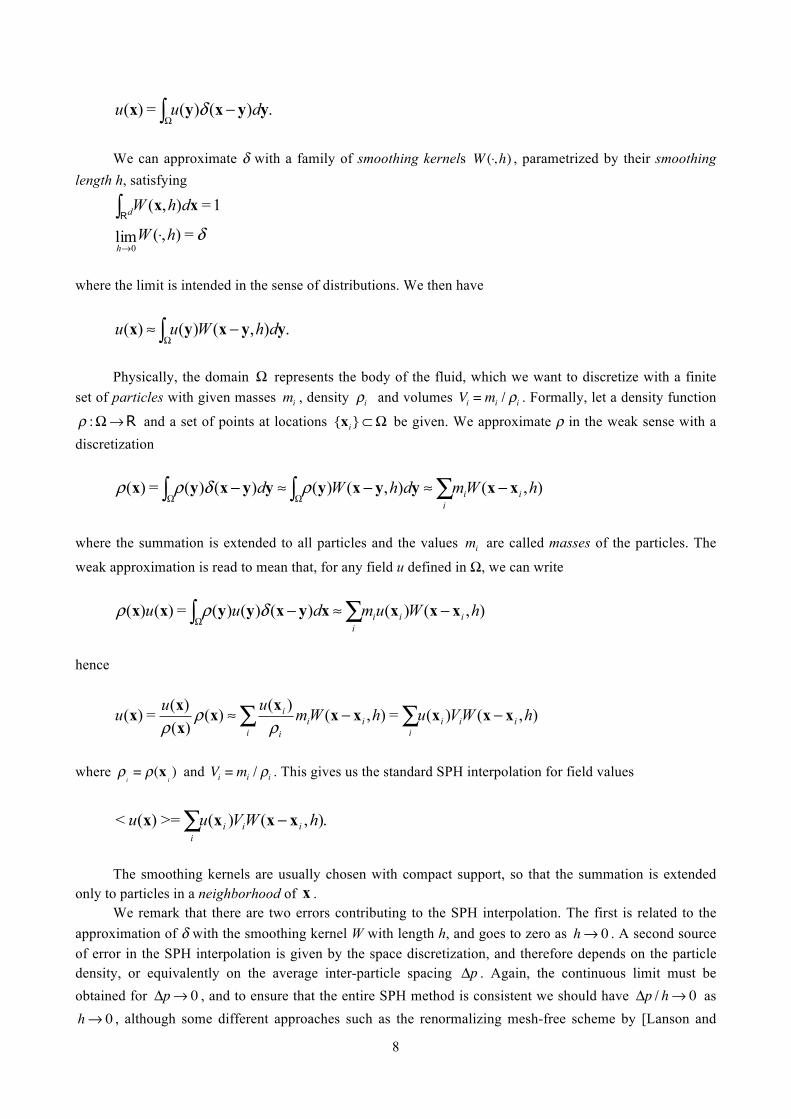
The mathematical foundation for SPH lies in the properties of convolutions. For any scalar field u in a domain Ω⊆Rd , by definition of the Dirac’s delta distribution δ we can write, with a typical abuse of notation,

8

.)()(=)( yyxyx duu −∫Ω δ

We can approximate δ with a family of smoothing kernels W (⋅,h) , parametrized by their smoothing

length h, satisfying

δ=),(lim

1=),(

0hW

dhW

h

d

⋅→

∫ xxR

where the limit is intended in the sense of distributions. We then have

.),()()( yyxyx dhWuu −≈ ∫Ω

Physically, the domain Ω represents the body of the fluid, which we want to discretize with a finite

set of particles with given masses mi , density ρi and volumes Vi = mi / ρi . Formally, let a density function

ρ :Ω→R and a set of points at locations {xi}⊂Ω be given. We approximate ρ in the weak sense with a discretization

),(),()()()(=)( hWmdhWd iii

xxyyxyyyxyx −≈−≈− ∑∫∫ ΩΩρδρρ

where the summation is extended to all particles and the values mi are called masses of the particles. The

weak approximation is read to mean that, for any field u defined in Ω, we can write

),()()()()(=)()( hWumduu iiii

xxxxyxyyxx −≈− ∑∫Ω δρρ

hence

),()(=),()()()()(=)( hWVuhWmuuu iii

iii

i

i

ixxxxxxx

xxx −−≈ ∑∑ ρ

ρρ

where ρ

i= ρ(x

i) and Vi = mi / ρi . This gives us the standard SPH interpolation for field values

.),()(>=)(< hWVuu iii

ixxxx −∑

The smoothing kernels are usually chosen with compact support, so that the summation is extended

only to particles in a neighborhood of x . We remark that there are two errors contributing to the SPH interpolation. The first is related to the

approximation of δ with the smoothing kernel W with length h, and goes to zero as h→ 0 . A second source of error in the SPH interpolation is given by the space discretization, and therefore depends on the particle density, or equivalently on the average inter-particle spacing Δp . Again, the continuous limit must be obtained for Δp→ 0 , and to ensure that the entire SPH method is consistent we should have Δp / h→ 0 as h→ 0 , although some different approaches such as the renormalizing mesh-free scheme by [Lanson and

9

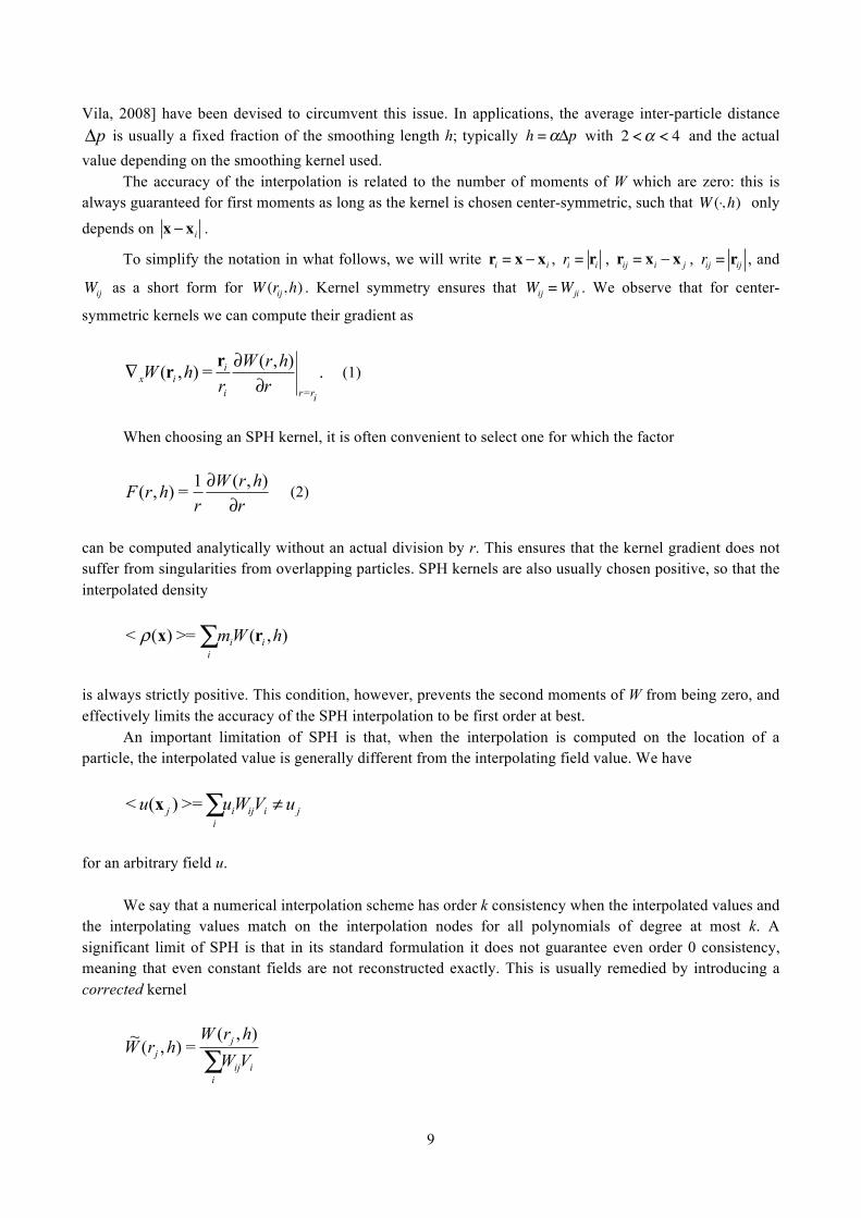
Vila, 2008] have been devised to circumvent this issue. In applications, the average inter-particle distance pΔ is usually a fixed fraction of the smoothing length h; typically h =αΔp with 2 <α < 4 and the actual

value depending on the smoothing kernel used. The accuracy of the interpolation is related to the number of moments of W which are zero: this is

always guaranteed for first moments as long as the kernel is chosen center-symmetric, such that W (⋅,h) only

depends on x − xi .

To simplify the notation in what follows, we will write ri = x − xi , ri = ri , rij = xi − x j , rij = rij , and

Wij as a short form for W (rij,h) . Kernel symmetry ensures that Wij =Wji . We observe that for center-

symmetric kernels we can compute their gradient as

.),(=),(= irri

iix r

hrWr

hW∂

∂∇ rr (1)

When choosing an SPH kernel, it is often convenient to select one for which the factor

rhrW

rhrF

∂∂ ),(1=),( (2)

can be computed analytically without an actual division by r. This ensures that the kernel gradient does not suffer from singularities from overlapping particles. SPH kernels are also usually chosen positive, so that the interpolated density

),(>=)(< hWm ii

irx ∑ρ

is always strictly positive. This condition, however, prevents the second moments of W from being zero, and effectively limits the accuracy of the SPH interpolation to be first order at best.

An important limitation of SPH is that, when the interpolation is computed on the location of a particle, the interpolated value is generally different from the interpolating field value. We have

jiijii

j uVWuu ≠∑>=)(< x

for an arbitrary field u.

We say that a numerical interpolation scheme has order k consistency when the interpolated values and

the interpolating values match on the interpolation nodes for all polynomials of degree at most k. A significant limit of SPH is that in its standard formulation it does not guarantee even order 0 consistency, meaning that even constant fields are not reconstructed exactly. This is usually remedied by introducing a corrected kernel

iiji

jj VW

hrWhrW

∑),(

=),(~

10

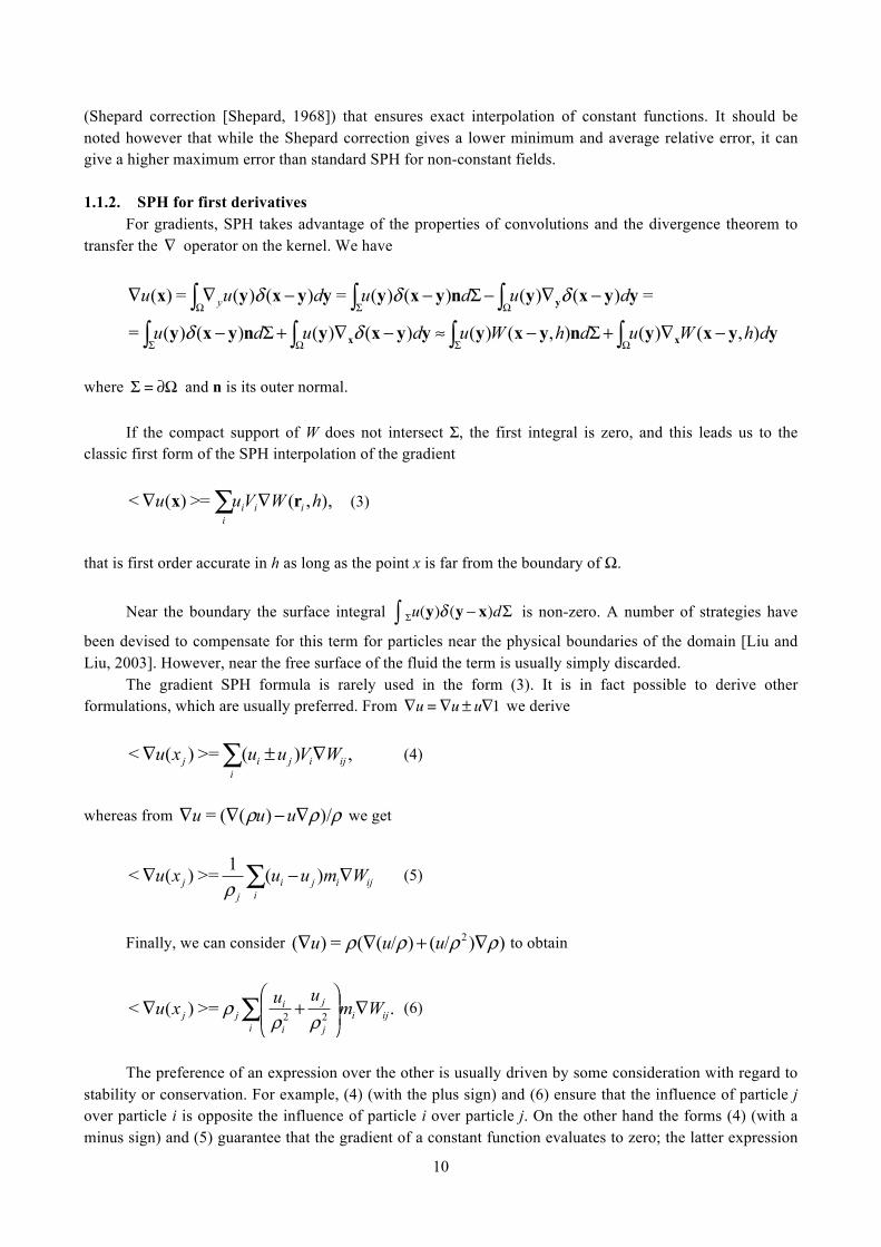
(Shepard correction [Shepard, 1968]) that ensures exact interpolation of constant functions. It should be noted however that while the Shepard correction gives a lower minimum and average relative error, it can give a higher maximum error than standard SPH for non-constant fields.

1.1.2. SPH for first derivatives

For gradients, SPH takes advantage of the properties of convolutions and the divergence theorem to transfer the ∇ operator on the kernel. We have

yyxynyxyyyxynyxy

yyxynyxyyyxyx

xx

y

dhWudhWududu

dududuu y

),()(),()()()()()(=

=)()()()(=)()(=)(

−∇+Σ−≈−∇+Σ−

−∇−Σ−−∇∇

∫∫∫∫∫∫∫

ΩΣΩΣ

ΩΣΩ

δδ

δδδ

where Σ = ∂Ω and n is its outer normal.

If the compact support of W does not intersect Σ, the first integral is zero, and this leads us to the

classic first form of the SPH interpolation of the gradient

),,(>=)(< hWVuu iiii

rx ∇∇ ∑ (3)

that is first order accurate in h as long as the point x is far from the boundary of Ω.

Near the boundary the surface integral Σ∫ u(y)δ (y − x)dΣ is non-zero. A number of strategies have

been devised to compensate for this term for particles near the physical boundaries of the domain [Liu and Liu, 2003]. However, near the free surface of the fluid the term is usually simply discarded.

The gradient SPH formula is rarely used in the form (3). It is in fact possible to derive other formulations, which are usually preferred. From ∇u =∇u ± u∇1 we derive

,)(>=)(< ijijii

j WVuuxu ∇±∇ ∑ (4)

whereas from ρρρ )/)((= ∇−∇∇ uuu we get

ijijiij

j Wmuuxu ∇−∇ ∑ )(1>=)(<ρ

(5)

Finally, we can consider ))/()/((=)( 2 ρρρρ ∇+∇∇ uuu to obtain

.>=)(< 22 ijij

j

i

i

ijj Wm

uuxu ∇⎟⎟⎠

⎞⎜⎜⎝

⎛+∇ ∑ ρρ

ρ (6)

The preference of an expression over the other is usually driven by some consideration with regard to

stability or conservation. For example, (4) (with the plus sign) and (6) ensure that the influence of particle j over particle i is opposite the influence of particle i over particle j. On the other hand the forms (4) (with a minus sign) and (5) guarantee that the gradient of a constant function evaluates to zero; the latter expression

11

is computationally more efficient, but the former is more stable in the case of large differences in the density values between particles, such as in the case of multiple fluids. Further details about the ‘golden rules’ of SPH can be found e.g. in [Monaghan, 1992].

1.1.3. SPH for second derivatives

Second-order derivatives can be derived in SPH using an approach similar to the one shown for first-order derivatives, but in the case of the Laplacian a different method is preferred. The method was first used by [Cleary and Monaghan, 1999] to model thermal conduction, and has been adapted by [Morris et al., 1997] for the dynamic case. It is derived from a Taylor expansion of the SPH gradient, and for a vector field )(xv it takes the form

ijijji

ijijjii

ij hr

Wm v

rv

)()(

>=< 222

ερρρρ

+∇⋅+

∇ ∑ (7)

where ε ≈ 0.01 and h is the smoothing length. The εh2 term is included to prevent singularities in the case of overlapping particles. In the case of symmetric (non-corrected) kernels, equation (1) can be used to simplify (7) to

ijji

ijjii

ij Fmv

ρρρρ v)(

>=< 2 +∇ ∑ (8)

where Fij = F(rij,h) with F defined as in (2). This expression has the benefit of being computable even in the

case of overlapping particles, provided that F can be computed analytically.

1.2. Navier-Stokes equations and their SPH discretization The Navier-Stokes equation, paired with a continuity equation for mass and either an incompressibility

condition or an equation of state that relates pressure to density, are the essential physical-mathematical model for fluid dynamics.

The classic application of SPH to computational fluid-dynamics discretizes the Navier-Stokes equations in the case of an isotropic, quasi-compressible fluid: the fluids are therefore assumed to be compressible, but with very small density fluctuations during their motion.

The equation of fluid motion we will take into consideration are therefore:

gvv +∇+∇− 2= νρP

DtD

(9)

,= v⋅∇−ρρDtD

(10)

,1=0

20

⎟⎟

⎠

⎞⎜⎜

⎝

⎛−⎟⎟⎠

⎞⎜⎜⎝

⎛γ

ρρ

γρ scP

12

where v represents the (Lagrangian) velocity, P the fluid pressure, ρ the fluid density and ρ0 the fluid density at rest; v is the kinematic viscosity coefficient. In our case, the external force, if present, will be gravity g = −gez with g = 9.81m2 / s and ez the unit vertical upwards vector; the cS coefficient in the equation of

state represents the speed of sound of the fluid at rest. SPH discretization of the right-hand side of each equation effectively turns the system of partial

differential equations into a system of ordinary differential equations in time. Specifically, assuming that F (2) can be computed analytically, the momentum equation (9)

traditionally takes the form

,= 22 gvv ++

+∇⎟⎟⎠

⎞⎜⎜⎝

⎛+−⎟

⎠⎞⎜

⎝⎛ ∑∑ ijij

ji

jij

jiji

i

i

j

jj

ji

FmWPPm

dtd

ρρµµ

ρρ (11)

where the viscous term is derived from equation (8) using the dynamic viscosity νρµ = .

A simpler form for the viscous term can be obtained by using the harmonic mean 2µiµ j / (µi + µ j ) of

the dynamic viscosities of the particles instead of their arithmetic mean (µi + µ j ) / 2 (see e.g. [Monaghan,

2005]), leading to the simplification:

jijiji

ji

jiji

ji

ρρν

ρρρρρρ

νρρµµ

µµ 4=14=14++

and a discretization of (9) in the form

.4= 22 gvv ++

+∇⎟⎟⎠

⎞⎜⎜⎝

⎛+−⎟

⎠⎞⎜

⎝⎛ ∑∑ ijij

jij

jiji

i

i

j

jj

ji

FmWPPm

dtd

ρρν

ρρ (12)

The formulation (12) , while simpler, can only be used single-fluid problems with a constant kinematic

viscosity. By contrast, formulation (11) is more appropriate for multi-fluid problems, or when the viscosity is not constant (e.g. thermal-dependent viscosity and/or non-Newtonian fluids [Hérault et al., 2011]).

For the continuity equation, there are also two common forms, specifically

ijiijjji

Wmdtd ∇⋅⎟

⎠⎞⎜

⎝⎛ ∑ v=ρ

(13)

and

.= ijiijj

j

ji

i

Wm

dtd ∇⋅⎟

⎠⎞⎜

⎝⎛ ∑ v

ρρρ (14)

Both formulations rely on the SPH discretization of the divergence operator

,>=< ijiijj

j

jW

m∇⋅−⋅∇ ∑ vv

ρ

13

which is derived in a manner similar to that seen in section 1.1 for the gradient. Again, the choice of the formulation can be problem dependent, with (14) preferred over the simpler

(13) in the case of large density variations, such as in the case of multiple fluids. An alternative to the use of the continuity equation is the so-called summation density approach: at

every time-step, the density of the i -th particle is reinitialized using its weak discretization:

.= ijjj

i Wm∑ρ (15)

Summation density is a simpler approach than the evolution equation derived from mass continuity,

and has the advantage of ensuring a better consistency between the geometrical density of the particles and the physical density of the fluid. However, it underestimates the particle density near the free surface, and it introduces a dependency of the particle density on the mass of the neighboring particles: the latter point is particularly a problem in case of multiple fluids with large differences in at-rest density.

1.3. Speed of sound in SPH

The weakly-compressible SPH method described in this chapter is typically used with an explicit time-stepping integration scheme. A significant consequence of this is that the speed of sound in the fluid can impose a very stringent condition on the maximum allowed time-step during the simulation.

In classical SPH, this is worked around by using a speed of sound for the fluid which is significantly lower than the physical speed of sound of the modeled fluid. This fictitious speed of sound is selected to be at least one order of magnitude higher than the maximum velocity expected during the simulation, to ensure that density fluctuations are kept small (typically within 1% of the reference density), while still achieving affordable simulation speeds.

2. SPH and parallel computing: GPUSPH When coupled with an explicit integration scheme, the SPH method becomes what is known as an

“embarrassingly parallel” problem. Indeed, the right-hand side of the ordinary differential equations in time shown at the end of the previous chapter (equations (12) and (13) in one formulation, equations (11) and (14) in the other) can be computed independently for each particle, knowing the current position, velocity and density of the particle itself as well as its neighbors (the pressure Pj of the j-th neighbor is obtained directly from its density ρj using the equation of state). In particular, no large, implicit systems of equations have to be assembled.

This direct computation of the forces for each particle, and the equally parallel nature of the integration steps, make it possible to implement SPH efficiently on high-performance parallel computing hardware, and particularly on Graphic Processing Unitcs (GPUs).

GPUs are video cards originally designed for the videogaming and computer-assisted design. Pushed by the growing interest for higher realism in video games, they have grown in computational power at faster rate than CPUs. This has elicited an interest of the scientific community for their use in scientific computing, resulting in the two major manufacturers exposing the computational capabilities of their GPUs for more generic applications than three-dimensional graphics, leading to the birth of what is known as GPGPU, General-purpose Programming on GPU.

A modern GPU has a theoretical computing performance that can match that of traditional CPU clusters, at a fraction of the cost, both in terms of initial investment and in terms of energy consumption.

14

However, the computing power of GPUs can only be exploited with massively parallel workloads, such as those of the weakly-compressible SPH numerical method.

The work presented in this report is implemented as an extension of GPUSPH, the first open source implementation of SPH on CUDA-enabled GPUs [Hérault et al., 2010]. In this chapter, an overall description of the GPUSPH structure is presented. This will serve as a reference for the implementation notes of the multi-fluid models presented in the next chapter.

2.1. GPUSPH structure

GPUSPH is a modular implementation of SPH on CUDA-enabled GPUs. Both the host side and the device side make heavy use of C++ template programing to provide a flexible, extensible structure that allows the implementation of multiple SPH formulations.

The fundamental classes used in GPUSPH are ParticleSystem and Problem. The Problem class is used to define the geometry and initial conditions of a simulation to be executed.

It also defines parameters such as the SPH formulation to be used, how often additional steps such as Shepard or MLS smoothing of the density are to be executed (if at all), how often the neighbor list must be rebuilt (see also section 2.1.2), and so on.

As the name suggests, the ParticleSystem abstracts the management of the system of particles resulting from the application of SPH to the Problem. This class handles the resources needed for the execution of a simulation (both on the host and on the GPU), and issues the actual computational steps needed for the time-stepping.

On the host, the allocated resources consist of an array each for the position, mass, velocity and density of all particles; an additional array is used to hold other identifying properties, such as a global particle identification number (which can be used to trace the motion of a single particle across the whole simulation), or flags to mark if a particle is a fluid particle or a boundary particle, or which object it belongs to. These arrays are initialized from values passed by the Problem, and are used again to retrieve data from the GPU when saving the results of a simulation.

The largest amount of memory, on the other hand, is allocated on the GPU. Indeed, due to the time-stepping scheme used, some of the arrays have to be duplicated, and additional ones are needed, as explained in the next section.

2.1.1. Integration scheme

GPUSPH uses a predictor-corrector integration scheme. With accelerations F and time-step dt, the scheme describing a time-step with the standard SPH formulation can be summarized as follows: 1) compute accelerations F (n) = F(x(n),v(n),ρ (n) ) and density derivatives ρ (n) = ρ(x(n),v(n),ρ (n) ) ;

2) compute half-step intermediate positions, velocities, densities:

a) 2

= )()()*( dtnnn vxx + ,

b) 2

= )()()*( dtF nnn +vv ,

c) 2

= )()()*( dtnnn ρρρ + ;

3) compute corrected accelerations ),,(= )*()*()*()*( nnnn FF ρvx and density derivatives

15

),,(= )*()*()*()*( nnnn ρρρ vx ;

4) compute new positions, velocities, densities:

a) dtdtF nnnn ⎟⎠⎞⎜

⎝⎛ +++

2= )*()()(1)( vxx ,

b) dtF nnn )*()(1)( = ++ vv ,

c) dtnnn )*()(1)( = ρρρ ++ .

From this, we see that on the GPU we need two arrays each for the particle position, mass, velocity,

density and extra information, plus an array to hold the forces computed at each partial step. Additionally, each particle needs to compute the maximum time-step allowed, based on the magnitude

of the force and the speed of sound. An array is used to collect all the values and then find the maximum allowed time-step (minimum of the array) using a parallel reduction.

Finally, an additional array holds, for each particle, a list of neighboring particles. This array, which is called the neighbor list, is crucial for performance reasons, but at the same time is the largest array used in the simulation.

2.1.2. The neighbor list

The neighbor list is a fundamental structure, needed to reduce the time spent in looking for particle neighbors during the simulation: a particle needs to iterate over its neighbors no less than once each force computation, so that it is faster to build a neighbor list once and then re-use it when needed.

Since the fluid is normally not subject to large instantaneous deformation, additional performance can be gained by rebuilding the neighbor list every n iterations instead of every iteration. This parameter can be configured at the Problem level.

The number of elements allocated for the neighbor list depends on the choices made for the radius of the smoothing kernel and on the smoothing length, as well as on the number of dimensions. For example, in three dimension, with a smoothing length of 1.3Δp and a kernel radius of 2 , each particle will typically have less than a hundred neighbors; in GPUSPH the limit in this case is actually set to 128 for safety reasons. For a kernel with radius 3 the maximum number of neighbors that can be expected for a particle is no less than 256, twice as much. Combined with the memory required by the particle data (position, mass, velocity, density) this leads to a requirement of over 1KB of memory per particle, most of which is used by the neighbor list.

Due to the upper limit of 6GB of memory on current GPUs, this effectively limits the maximum number of particles in GPUSPH to less than 5 million particles when using kernels with radius 3, and almost 8 million particles when using kernels with radius 2.

To work around this limitation, it is necessary to extend GPUSPH to use multiple devices. A multi-GPU version of GPUSPH is already available [Rustico et al., 2014], and a multi-node implementation that would allow the distribution of computation across multiple nodes in a cluster, each with multiple GPUs, is also currently under development.

2.1.3. Boundary conditions

GPUSPH implemented three different approaches to boundary conditions on physical boundaries: Lennard-Jones particles, Monaghan-Kajtar particles, and geometrical boundaries.

16

Lennard-Jones particles are the classic approach to boundary particles in SPH: physical boundaries are filled with one layer of equally spaced particles that exert a Lennard-Jones force on fluid particles. A known problem of this approach is that a particle travelling parallel to a plane does not perceived a constant repulsive force, due to pockets of potential between particles.

Monaghan and Kajtar [Monaghan and Kajtar, 2009] offered a solution to this problem by filling the boundary planes with a more tightly spaced grid of particles, a process that significantly reduce the influence of potential pockets, at the cost of a significantly higher number of boundary particles.

Finally, the third option included in GPUSPH describes the boundary geometrically. During force computation, each particle then computes its distance from the boundaries and, if the distance is less than a given threshold, a Lennard-Jones force is exerted perpendicularly to the boundary. This approach is efficient, since no boundary particles are needed, and it ensures that the force exerted on a particle travelling parallel to a plane is constant. In GPUSPH, geometrical boundaries are implemented for planes, used to describe simple, regular geometries, and for Digital Elevation Models, used to describe more complex geometries such as natural topographies.

The semi-analytical boundary conditions of Ferrand et al. [Ferrand et al., 2013], which provide a more accurate wall treatment, has also been recently introduced in a development branch of GPUSPH [Vorobyev, 2013]. Since the implementation has proceeded in parallel with the work presented here, the integration of this boundary model with our multi-fluid work remains a prospective for future work (see also section 5.2).

3. Multi-fluid SPH models

3.1. Introduction The classical SPH formulation presented in section 1.1 presents a number of issues when applied to

multi-fluid problems naively. In particular, large density ratios and large differences in mass distribution among particles can introduce significant numerical instabilities, especially near the interface between multiple fluids. Even the formulas which are more appropriate for large density variations fail to behave correctly when the differences are of one order of magnitude or more (such as, for example, in the case of air water simulations).

A possible solution to this issue is to move from a density-based formulation to one based on volumes. Different approaches are possible, and we will present here two of them, one proposed by Hu & Adams [2006], and the other by Grenier [Grenier et al., 2008; 2009; Grenier, 2009].

3.2. Hu & Adams multi-fluid model

3.2.1. Formulation

The SPH formulation proposed by Hu & Adams [2006] relies on the introduction of the quantity

)(=)( jjW xxx −∑σ (16)

where W is the usual SPH smoothing kernel and the summation, as usual, is extended over all particles within the influence radius of position x. It can be shown that for a particle i we have σ i ≡σ (xi ) ≈1/Vi where Vi is the particle volume, by considering the Shepard-corrected characteristic functions:

)()(=)(j

j

ii W

Wxxxxx−−

∑χ

17

and observing that

iiii dWdV

σσχ 1)(

)(1=)( ≈−≈ ∫∫ ΩΩ

xxxx

xx

where the last equality comes from the approximating properties of W. This equivalence allows Hu & Adams to replace the density evolution equation with

,= iii mσρ (17)

using an approach that is similar to the standard summation density approach (15), without the issues related to having contributions from the masses of other particles, and with the usual caveat that the approximation is correct only when the support of the kernel is complete.

By using (17), the pressure contribution for the momentum equation can then be rewritten as

ijij

j

i

i

ji

WPP

m∇⎟⎟⎠

⎞⎜⎜⎝

⎛+− ∑ 22

1σσ

(18)

while the viscous force in Hu & Adams formulation is given by

.112122 ijijjiji

ji

ji

Fm

v⎟⎟⎠

⎞⎜⎜⎝

⎛+

+∑ σσµµµµ

(19)

3.2.2. Boundary conditions and ghost particles Since the approximation of the inverse volume with σ is only valid when the support of the kernel is

complete, Hu & Adams formulation cannot be used as-is for free surface flows, as remarked also by [Monaghan & Rafiee, 2012] in proposing their alternative approach.

For solid boundaries, Hu & Adams propose the use of the ghost particles approach. When a solid boundary intersects the kernel support for a particle, a virtual particle mirror of the real particle is created across the solid boundary. The virtual (or ghost) particle will have the same mass, volume and density as its real counterpart, and a velocity which is opposite the original velocity in case of no-slip boundary conditions, or symmetric in the case of free-slip boundary conditions.

Hu & Adams point out in their work that this approach can only reliably be used in the case of planar walls, which is sufficient in most of our test cases. Additionally, no details are discussed in Hu & Adams’ paper about the treatment of corners, for which we developed our own strategy, limited to the case of rectangular domains. The use of a more sophisticated wall mode, such as one based on Ferrand’s semi-analytical boundaries, would lift this restriction on the domain geometry (see also section 5.2).

In two dimensions, the geometry of the domain is assumed to be a rectangle, whose sides are described by known linear equations. In such a case, a real particle P will have:

• one ghost if the kernel support intersects a single side; • three ghosts if the kernel support intersects two sides: the virtual particles symmetric of P across each

of the two sides, plus the virtual particle symmetric of P across the corner (intersection of the two sides).

18

In three dimensions, the geometry of the domain is assumed to be a rectangular parallelepiped. In such a case, a real particle P will have:

• one ghost if the kernel support intersects a single side; • three ghosts if the kernel support intersects two sides: the virtual particles symmetric of P across each

of the two sides, plus the virtual particle symmetric of P across the edge (intersection of the two sides);

• seven ghosts if the kernel support intersects three sides: the virtual particles symmetric of P across each of the three sides, plus the virtual particles symmetric of P across each of the three edges (intersection of each pair of sides), and finally a virtual particle symmetric of P across the vertex (intersection of the three edges).

3.2.3. Implementation notes GPUSPH, which we used as a basis for our implementation of Hu & Adams’ formulation, already

includes infrastructure to allow the use of multiple fluids with different properties (density and sound-speed), although it was necessary to extend this to include support for different viscosity coefficients.

GPUSPH also includes infrastructure to support multiple formulations. The actual formulation to be used during a single simulation is defined by the Problem. Our addition of Hu & Adams’ formulation makes it selectable using the SPH_HU_ADAMS value for the formulation.

When the Hu & Adams’ formulation is selected, the appropriate discretized equations are used during force computation. Additionally, in this case an extra computational step is inserted the GPUSPH pipeline. The original integration scheme presented in section 2.1.1 is then modified, when using Hu & Adams’ formulation, by replacing the integration steps for the density with the computation of σ. Specifically, the integration scheme now becomes:

1) compute accelerations ),,(= )()()()( nnnn FF σvx ;

2) compute half-step intermediate positions, velocities, inverse volumes:

a) 2

= )()()*( dtnnn vxx + ,

b) 2

= )()()*( dtF nnn +vv ,

c) )(= )*()*( nn xσσ ;

3) compute corrected accelerations ),,(= )*()*()*()*( nnnn FF σvx ;

4) compute new positions, velocities, inverse volumes

a) dtdtF nnnn ⎟⎠⎞⎜

⎝⎛ +++

2= )*()()(1)( vxx ,

b) dtF nnn )*()(1)( = ++ vv ,

19

c) )(= 1)(1)( ++ nn xσσ .

Initialization During initialization, it is necessary to ensure that the particle distribution and the assigned masses and

volumes are coherent. The particle distribution that is usually chosen at problem set-up consists of a regular grid of equally-spaced particles, which leads to a uniform initial geometrical volume or, equivalently, to all particles having the same σ as computed from (16).

This leads to a uniform initial pressure, which causes a vertical collapse of the particles in the initial phases of the simulation, as the fluids tries to achieve hydrostatic pressure balance. This is a well-known phenomenon in weakly-compressible SPH simulations, the solution to which is to ensure that the initial pressure distribution counter-balances the hydrostatic pressures.

When the formulation by Hu & Adams is being used, this can only by achieved by either using a non-regular initial distribution of particles, or by altering the particle masses so that the initial densities lead to a hydrostatic pressure distribution, a process which leads to a slight increase in total fluid mass.

Boundary conditions

The ghost particles boundary method was developed as an additional approach to realize physical boundaries in GPUSPH. The planes bounding the computational domain are described using the same form used for the geometrical boundaries already implemented in GPUSPH. However, instead of a virtual particle exerting a Lennard-Jones force, the planes are used to generate ghosts of each neighbors of a particle whose kernel intersects one or more planes.

The ghosts are generated dynamically during force computation, so they do not occupy additional memory. The current implementation, while robust, is not particularly efficient, and has a significant impact on the performance of the code and thus the run-times of the simulations.

3.3. Grenier’s multi-fluid model

3.3.1. Formulation

The core principle behind Grenier’s model for multi-fluid Grenier [Grenier et al., 2008; 2009; Grenier, 2009]. is similar to the one used by Hu & Adams, i.e. to use volumes instead of densities as fundamental particle properties.

In contrast to Hu & Adams, however, Grenier uses the actual particle volume ω instead of a discretized approximation of its inverse. The continuity equation is written in terms of the Jacobian

J = ωω 0 =

ρ0

ρ, where ω0 and ρ0 denote the initial value of the particle’s volume and density, respectively.

The continuity equation (10) now takes the analytical form

,=log v⋅∇DtJD

which is discretized with the Shepard-corrected divergence

),()(1=logjij

jW

DtJD xxvv −∇⋅−∑σ

20

where σ is defined as in (16). It should be noted however that while the expression of σ formally matches the one used in Hu & Adams, its physical meaning is not directly related to the inverse volume anymore.

The density ρi of a particle is computed as a smoothed mass M divided by the particle volume, where

M is computed with a Shepard-corrected kernel limited to the particles belonging to the same fluid:

i

ii

ik

iKk

ikk

iKki

MW

WmM

ωρ =,=

∑∑

∈

∈ (20)

where Ki is the set of indices of particles having the same fluid type as particle i. If all particles belonging to the same fluid have the same mass, the smoothing can be skipped as it’s algebraically equal to the particle mass mi.

For the momentum equation, the pressure contribution is then given by

ijij

j

i

i

ji

WPP ∇⎟

⎟⎠

⎞⎜⎜⎝

⎛+− ∑ σσρ

1

while the viscous force is given by

.1121ijij

jiji

ji

ji

F v⎟⎟⎠

⎞⎜⎜⎝

⎛+

+∑ σσµµµµ

ρ These expressions are closely related to (18) and (19) respectively, except for a factor σ inside and

outside the summation. The difference between the two methods therefore grows more noticeable as the difference in volumes between adjacent particles grows larger.

3.3.2. Boundary conditions and surface tension

The leading difference between Hu & Adams’ formulation and Grenier’s is that the latter can be reliably used also for free-surface flows, thanks to the use of a continuity equation for the volume and the use of the Shepard-corrected smoothed mass in the computation of the particle densities. For physical boundaries, the use of ghost particles is still the preferred approach, as it leads to a smoother evolution of the particle volumes compared to e.g. the approach with Lennard-Jones particles.

Both Hu & Adams and Grenier also present a model for surface tension. These models are appropriate for problems in which surface tension is a dominant factor in fluid evolution (e.g. oil/water simulations), and were thus beyond the scope of this project.

Grenier also introduced a simplified surface tension model. This model was implemented to allow the validation of our implementation against Grenier’s own results, and in some cases we could see that it was indeed a necessary addition to the model (see for example section 4.5.2)

In the simplified model, surface tension is modeled as an additional component to the pressure discretization:

ijij

j

i

i

iOjIiji

j

j

i

i

ji W

PPWPPP ∇⎟

⎟⎠

⎞⎜⎜⎝

⎛++∇⎟

⎟⎠

⎞⎜⎜⎝

⎛+∇ ∑∑

∈ σσε

σσ>=)(< x

21

where the second sum is extended to all neighbor particles which are of a different fluid (i.e. the complementary set to the Ki used in (20)).

Although the simplified model for surface tension is not able to reproduce correctly the behavior of the surface when the tension effect is strong, it helps in smoothing out the interface between two fluids during normal evolution. The dimensionless coefficient εI should be chosen small enough to provide the smoothing effect without altering the fluid behavior, and typically ranges from 0.01 to 0.1.

3.3.3. Implementation notes

Our implementation of Grenier’s formulation can be selected in GPUSPH by giving the value SPH_GRENIER as the formulation parameter in the Problem. Aside from switching to the appropriate discretization formulas during force computation, choosing Grenier’s formulation also introduces a new steps in the GPUSPH integration scheme described in section 1.1, to compute the smoothed density and the value of σ for each particle.

To simplify notation, set L = log J and let L be its derivative in time, computed from Grenier’s

continutiy equation. Since the computation of ρ is still required to compute the pressure, the integration scheme is now slightly more complex than the one used for standard SPH or the one used for Hu & Adams. Specifically, the steps are now:

1) compute accelerations F (n) = F(x(n),v(n),ρ (n),σ (n) ) and log-Jacobian derivatives L(n) = L(x(n),v(n),σ n ) ;

2) compute half-step intermediate positions, velocities, volumes, densities, σ:

a) 2

= )()()( dtnnn vxx +* ,

b) 2

= )()()*( dtF nnn +vv ,

c) 2

= )()()*( dtLLL nnn + , 0)*()*( )(exp= ωω nn L and )()*( /= *nn M ωρ ,

d) )(= )*()*( nn xσσ ;

3) compute corrected accelerations ),,,(= )*()*()*()*()*( nnnnn FF σρvx and log-Jacobian derivatives

),,(= *)(*)()*()*( nnnn LL σvx ;

4) compute new positions, velocities, volumes, densities, σ:

a) dtdtF nnnn ⎟⎠⎞⎜

⎝⎛ +++

2= )()()(1)( *vxx ,

b) dtF nnn )*()(1)( = ++ vv ,

c) dtLLL nnn 1)()(1)( = ++ + , 01)(1)( )(exp= ωω ++ nn L , and 1)(1)( /= ++ nn M ωρ ,

22

d) )(= 1)(1)( ++ nn xσσ . The implementation has been factorized so that it should be possible, with minimal effort, to produce

a new model based on a combination of Grenier’s and Hu & Adams’ formulations, for example by introducing a density evolution or the simplified surface tension in Hu & Adams’ model.

4. Validation

4.1. Introduction

4.1.1. Description of the test cases Validation of our implementation of Hu & Adams’ (section 3.2) and Grenier’s (section 3.3) models

has been done on a number of different scenarios, both in two and three dimensions.

Rayleight-Taylor instability: this is a classic problem, with a heavier fluid resting on top of a lighter fluid, with an initially perturbed surface; the gravity force then leads to fluid mixing at a speed related to the density ratio of the fluids;

Lock exchange: this problem, also known as gravity current, presents itself as a box filled with two fluids side by side, separated by a barrier; as the barrier is removed, the heavier fluid flows below the lighter fluid, presenting a characteristic hydraulic jump at the head of the flow;

Rising bubble: in this problem, a spherical air bubble floats towards the surface of a water-filled container, leading to a characteristic deformation of the bubble shape, reaching the point of fracture.

The Rayleigh-Taylor in two dimensions is considered a classic benchmark in multi-fluid CFD,

although comparison is only possible against other numerical codes. The lock exchange problem has been thoroughly studied, and it is possible to compare the results both against physical experiments and against theoretical results. For us, this has been one of the most extensive validation tests, although limited to small density ratios. Finally, The rising bubble test has allowed us to assess the behavior of the models with density ratios as high as 103. In the two-dimensional case the validation was done against Grenier’s own implementation, while for the three-dimensional case only a more qualitative analysis of the behavior was possible. 4.2. Smoothing kernels

Two smoothing kernels are used in the validation tests, a Wendland kernel with radius 2 and analytical expression for the factor F (2) , and a normalized Gaussian kernel with radius 3.

The Wendland kernel is based on the ψ3,1 function defined by [Wendland, 1995], with W (r,h) = w(r / h) / hd where d is the space dimension (in our case 2=d or 3 ), and

⎪⎩

⎪⎨⎧

≤+⎟⎠⎞⎜

⎝⎛ −

2;>0

21)(22

1=)(

4

q

qqqKqw w

the resulting gradient factor can then be written as 2)//(=),( +dhhrfhrF with

23

,2>022)(

=)(3

⎩⎨⎧ ≤−

qqqK

qf f

so that ∇W (xij,h) = xijF(rij,h) . The normalization constants are dimension-dependent as well: for d = 2 we

have Kw =74π

, K f =3532π

, whereas for d = 3 we have Kw =2116π

and K f =105128π

.

The Gaussian kernel is taken from Grenier [Grenier et al., 2008], and it has the form W (r,h) = w(r / h)

where

⎪⎩

⎪⎨⎧

≤−−−

,>0

)(exp)(exp=)(

22

kq

kqC

kqqw

where k is the kernel (cut-off) radius and C is the normalization constant. The corresponding gradient factor takes the form 2)//(=),( +dhhrfhrF where

⎩⎨⎧ ≤−−

kqkqqQ

qf>0

)(exp=)(

2

and Q = 2 /C . In two dimensions we have C = π (1− exp(−k2 )(1+ k2

)) , while in three dimensions

C = π 3 erf(k)− 2π exp(−k2 )k(3+ 2k2 ) / 3 . The Gaussian kernel can be used with a variety of radii. We follow Grenier, and use K = 3 in all our tests.

4.3. Rayleigh-Taylor instability

Validation for the Rayleigh-Taylor instability has been done using the same two-dimensional problem set-up described by [Grenier et al., 2009].

The computational domain is rectangular, with a width (x direction) L =1m and a height (z direction) of 2L. The two fluids are separated by an interface located at z =1− 0.15 ⋅sin(2π x) . The two fluids have a density ratio of 1.8.

L 1 Re 420 ratioρ 1/1.8

Iε 0.01 Kernel Gaussian Radius 3

Light fluid Heavy fluid

ρ ( 3m/kg ) 1 1.8 γ 7 7 c ( s/m ) 62.642 62.642

ν ( s/m2 ) 3107.46 −⋅ 3107.46 −⋅

Table 1. Summary of parametes used in the validation of the Rayleigh-Taylor problem.

24

In our equations of state, we set γ = 7 and, expecting a maximum velocity vmax = gL , assign a speed

of sound (at rest) of c = 20 vmax for both fluids. Similarly, the same viscosity is assumed for both fluids,

computed from the assigned Reynolds number Re = vmax ⋅L /ν = 420 . No-slip boundary conditions are imposed at the boundaries, using ghost-particles with opposite velocities.

Our initial setup places the particles on a regular square lattice, with particles marked as belonging to one fluid or the other depending on their (x,z) coordinates. Constant pressure with at-rest density is used as initial condition. For all our tests here we used a linear resolution given by /300L , giving about 180 thousand particles.

Following Grenier et al. [2009], our figures will show the evolution of the simulation at times t*,3t*,5t * where t* = L / g is the characteristic time scale. The comparison with Grenier’s own result can

be found in section 4.3.3. A summary of the parameters used in the final validations is shown in Table 1.

4.3.1. Hu & Adams’ formulation Our first set of results is given by the Rayleigh-Taylor problem solved using Hu & Adams’ approach,

with both the Wendland kernel of radius 2 (Figure 1) and the Gaussian kernel of radius 3 (Figure 2).

*= tt *3= tt *5= tt

Figure 1. Evolution of the two-dimensional Rayleigh-Taylor problem, obtained with our implementation of Hu & Adams’ method and using the Wendland kernel. Particles are colored by fluid number.

25

*= tt *3= tt *5= tt

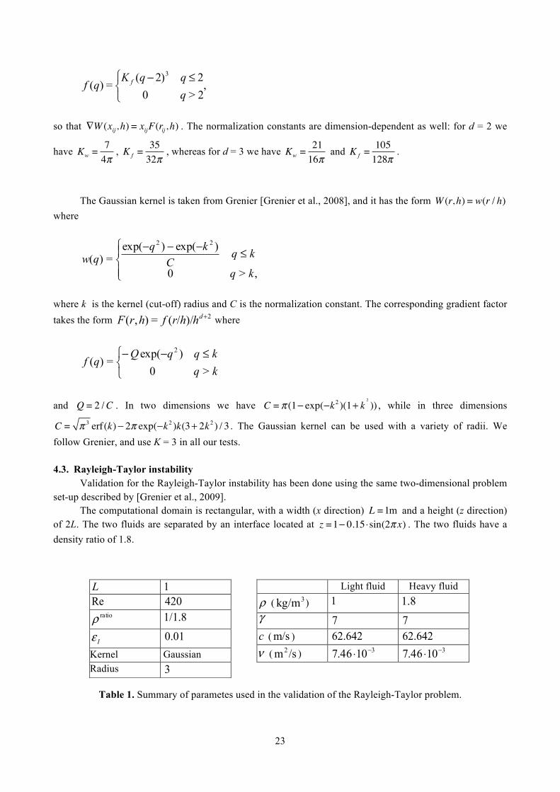
Figure 2. Evolution of the two-dimensional Rayleigh-Taylor problem, obtained with our implementation of Hu & Adams’ method and using the Gaussian kernel. Particles are colored by fluid number.

The most noticeable result in this comparison is the huge influence that the choice of smoothing kernel

has on the simulation: using the Gaussian kernel with radius 3 allows us to recover the expected shape of the interface, while the Wendland kernel with radius 2 introduces a strong numerical viscosity in the simulation, resulting in a significantly delayed progress in the flow.

We can also observe a minor perturbation on the top surface of the tank, due to the initial vertical collapse of the particles, a well-known phenomenon observed in SPH simulations. The influence of this effect on the flow however is small, making it unnecessary, in this case, to use alternative initializations procedures (such as assigning an initial hydrostatic pressure).

4.3.2. Grenier’s formulation

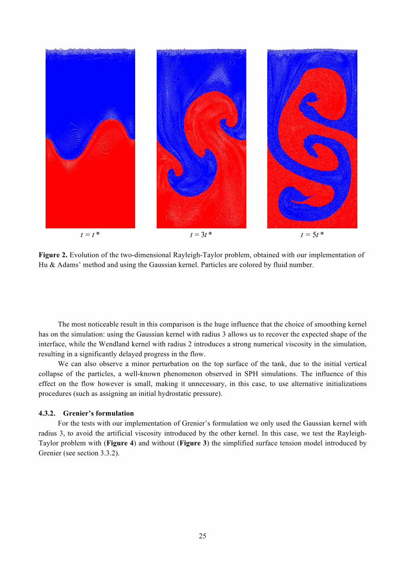
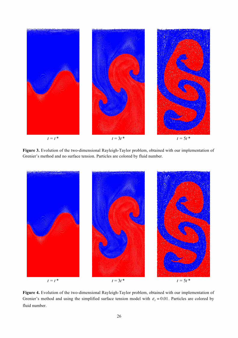
For the tests with our implementation of Grenier’s formulation we only used the Gaussian kernel with radius 3, to avoid the artificial viscosity introduced by the other kernel. In this case, we test the Rayleigh-Taylor problem with (Figure 4) and without (Figure 3) the simplified surface tension model introduced by Grenier (see section 3.3.2).

26

*= tt *3= tt *5= tt

Figure 3. Evolution of the two-dimensional Rayleigh-Taylor problem, obtained with our implementation of Grenier’s method and no surface tension. Particles are colored by fluid number.

*= tt *3= tt *5= tt

Figure 4. Evolution of the two-dimensional Rayleigh-Taylor problem, obtained with our implementation of Grenier’s method and using the simplified surface tension model with ε I = 0.01 . Particles are colored by fluid number.

27

We observe that we manage to reproduce the expected flow behavior and, as expected by the theory, we see that the introduction of the surface tension does not alter the fluid flow in a significant way.

w/o surface tension with surface tension

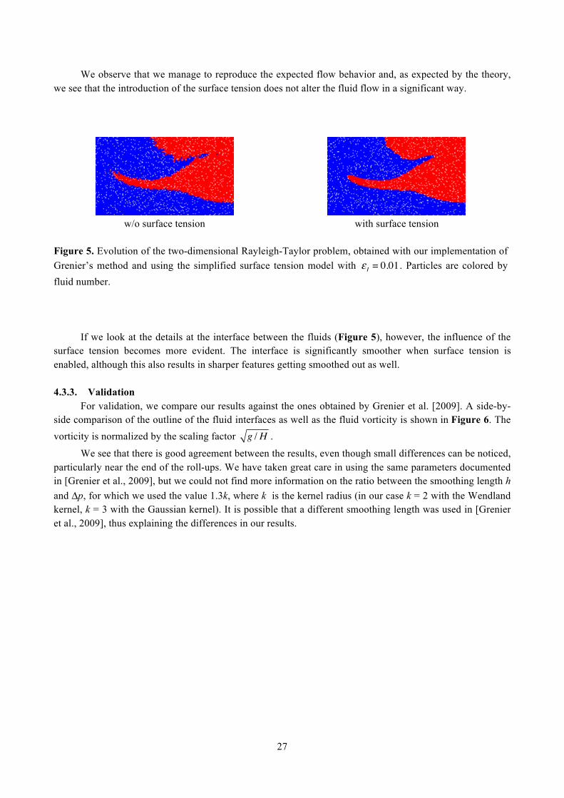
Figure 5. Evolution of the two-dimensional Rayleigh-Taylor problem, obtained with our implementation of Grenier’s method and using the simplified surface tension model with ε I = 0.01 . Particles are colored by fluid number.

If we look at the details at the interface between the fluids (Figure 5), however, the influence of the

surface tension becomes more evident. The interface is significantly smoother when surface tension is enabled, although this also results in sharper features getting smoothed out as well.

4.3.3. Validation

For validation, we compare our results against the ones obtained by Grenier et al. [2009]. A side-by-side comparison of the outline of the fluid interfaces as well as the fluid vorticity is shown in Figure 6. The vorticity is normalized by the scaling factor g /H .

We see that there is good agreement between the results, even though small differences can be noticed, particularly near the end of the roll-ups. We have taken great care in using the same parameters documented in [Grenier et al., 2009], but we could not find more information on the ratio between the smoothing length h and Δp, for which we used the value 1.3k, where k is the kernel radius (in our case k = 2 with the Wendland kernel, k = 3 with the Gaussian kernel). It is possible that a different smoothing length was used in [Grenier et al., 2009], thus explaining the differences in our results.

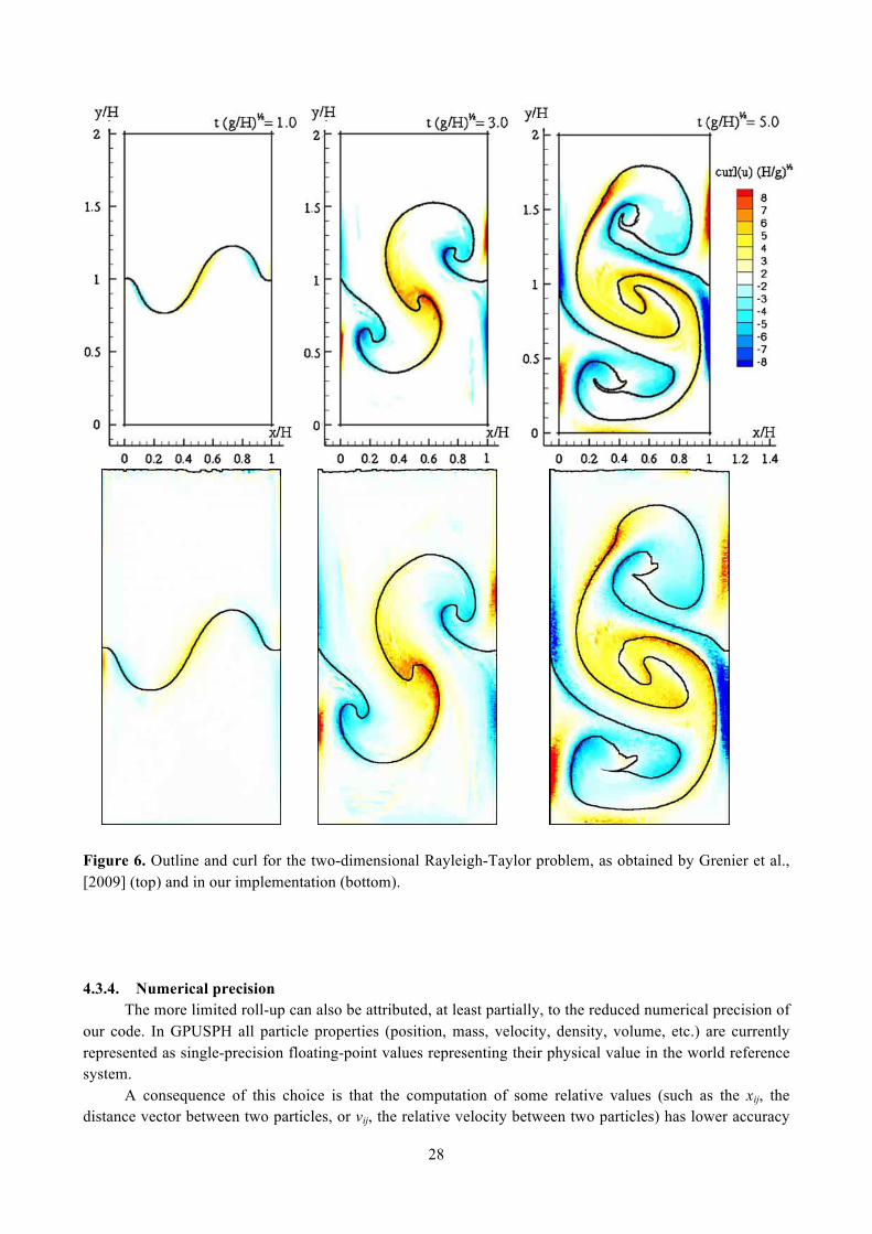
28

Figure 6. Outline and curl for the two-dimensional Rayleigh-Taylor problem, as obtained by Grenier et al., [2009] (top) and in our implementation (bottom).

4.3.4. Numerical precision The more limited roll-up can also be attributed, at least partially, to the reduced numerical precision of

our code. In GPUSPH all particle properties (position, mass, velocity, density, volume, etc.) are currently represented as single-precision floating-point values representing their physical value in the world reference system.

A consequence of this choice is that the computation of some relative values (such as the xij, the distance vector between two particles, or vij, the relative velocity between two particles) has lower accuracy

29

as the absolute values grow larger. For example, the distance vector is less accurate in areas further from the origin of the reference system, and the relative velocity is less accurate for particles with high velocity.

This phenomenon does not usually have a significant impact on a simulation; however, for larger domains it can undermine the capability of the model to represent finer details.

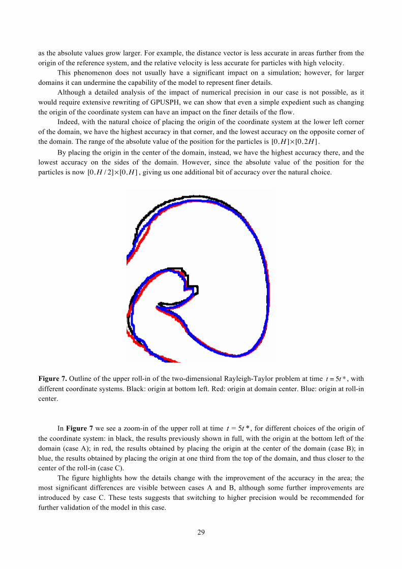
Although a detailed analysis of the impact of numerical precision in our case is not possible, as it would require extensive rewriting of GPUSPH, we can show that even a simple expedient such as changing the origin of the coordinate system can have an impact on the finer details of the flow.

Indeed, with the natural choice of placing the origin of the coordinate system at the lower left corner of the domain, we have the highest accuracy in that corner, and the lowest accuracy on the opposite corner of the domain. The range of the absolute value of the position for the particles is [0,H ]× [0, 2H ] .

By placing the origin in the center of the domain, instead, we have the highest accuracy there, and the lowest accuracy on the sides of the domain. However, since the absolute value of the position for the particles is now [0,H / 2]× [0,H ] , giving us one additional bit of accuracy over the natural choice.

Figure 7. Outline of the upper roll-in of the two-dimensional Rayleigh-Taylor problem at time t = 5t * , with different coordinate systems. Black: origin at bottom left. Red: origin at domain center. Blue: origin at roll-in center.

In Figure 7 we see a zoom-in of the upper roll at time *5= tt , for different choices of the origin of

the coordinate system: in black, the results previously shown in full, with the origin at the bottom left of the domain (case A); in red, the results obtained by placing the origin at the center of the domain (case B); in blue, the results obtained by placing the origin at one third from the top of the domain, and thus closer to the center of the roll-in (case C).

The figure highlights how the details change with the improvement of the accuracy in the area; the most significant differences are visible between cases A and B, although some further improvements are introduced by case C. These tests suggests that switching to higher precision would be recommended for further validation of the model in this case.

30

4.4. Lock exchange / Gravity current The lock exchange is our first fully three-dimensional validation test. Following [Lowe et al., 2005],

our domain is a box which is H = 0.2m tall, 1.82m wide and 0.23m deep. The domain is divided in half by a gate, and each half is filled with a different liquid. The gate is removed (in theory, instantly), causing the heavier fluid to flow below the lighter fluid.

H 2.0 Re 95500 ratioρ 0.681

Iε 0.01 Kernel Gaussian Radius 3

Light fluid Heavy fluid ρ ( 3m/kg ) 1000 1468.43 γ 7 7 c ( s/m ) 28.014 28.014 ν ( s/m2 ) 610− 610−

Table 2. Summary of parametes used in the validation of the Lock Exchange (gravity current) problem.

In Lowe’s experiments, the low density fluid is fresh water with density ρ0 =1000kg / m3 , and the

denser fluid is a solution with NaCl or NaI, with different concentrations to achieve different density ratios. We focus our validation test on a density ratio ρ ratio = 0.681 . In GPUSPH we assume both fluids have the

same equation of state with exponent γ = 7 and sound speed c0 = 20vmax with vmax = gH . The

dimensionless time coefficient is

t* = Hg ⋅(1− ρ ratio )

.

A summary of the parameters used in the validation is shown in Table 2.

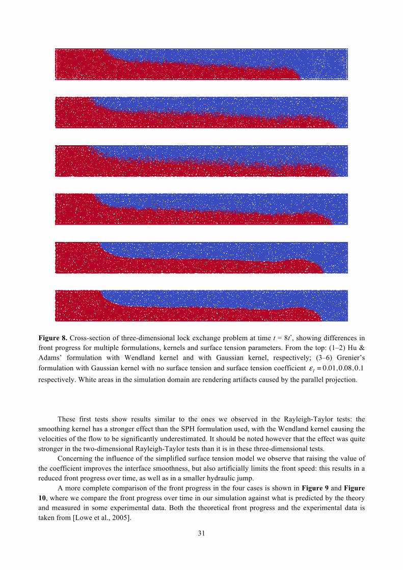
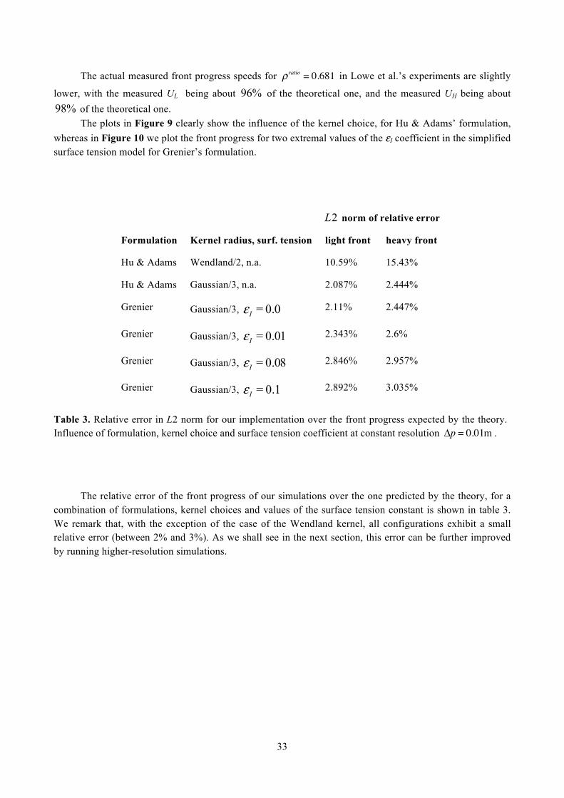
4.4.1. Influence of formulation and surface tension In Figure 8 we show a cross section of the three-dimensional lock exchange problem at time t = 8t* .

From the top we have: Hu & Adams’ formulation, with Wendland and Gaussian kernel respectively, followed by Grenier’s formulation with Gaussian kernel and four different values for the coefficient of the simplified surface tension model: ε I = 0 (no surface tension), ε I = 0.01, 0.08, 0.1 respectively. All these simulations were done with Δp = 0.01m , resulting in about 80 thousand particles.

31

Figure 8. Cross-section of three-dimensional lock exchange problem at time t = 8t*, showing differences in front progress for multiple formulations, kernels and surface tension parameters. From the top: (1–2) Hu & Adams’ formulation with Wendland kernel and with Gaussian kernel, respectively; (3–6) Grenier’s formulation with Gaussian kernel with no surface tension and surface tension coefficient ε I = 0.01, 0.08, 0.1 respectively. White areas in the simulation domain are rendering artifacts caused by the parallel projection.

These first tests show results similar to the ones we observed in the Rayleigh-Taylor tests: the

smoothing kernel has a stronger effect than the SPH formulation used, with the Wendland kernel causing the velocities of the flow to be significantly underestimated. It should be noted however that the effect was quite stronger in the two-dimensional Rayleigh-Taylor tests than it is in these three-dimensional tests.

Concerning the influence of the simplified surface tension model we observe that raising the value of the coefficient improves the interface smoothness, but also artificially limits the front speed: this results in a reduced front progress over time, as well as in a smaller hydraulic jump.

A more complete comparison of the front progress in the four cases is shown in Figure 9 and Figure 10, where we compare the front progress over time in our simulation against what is predicted by the theory and measured in some experimental data. Both the theoretical front progress and the experimental data is taken from [Lowe et al., 2005].

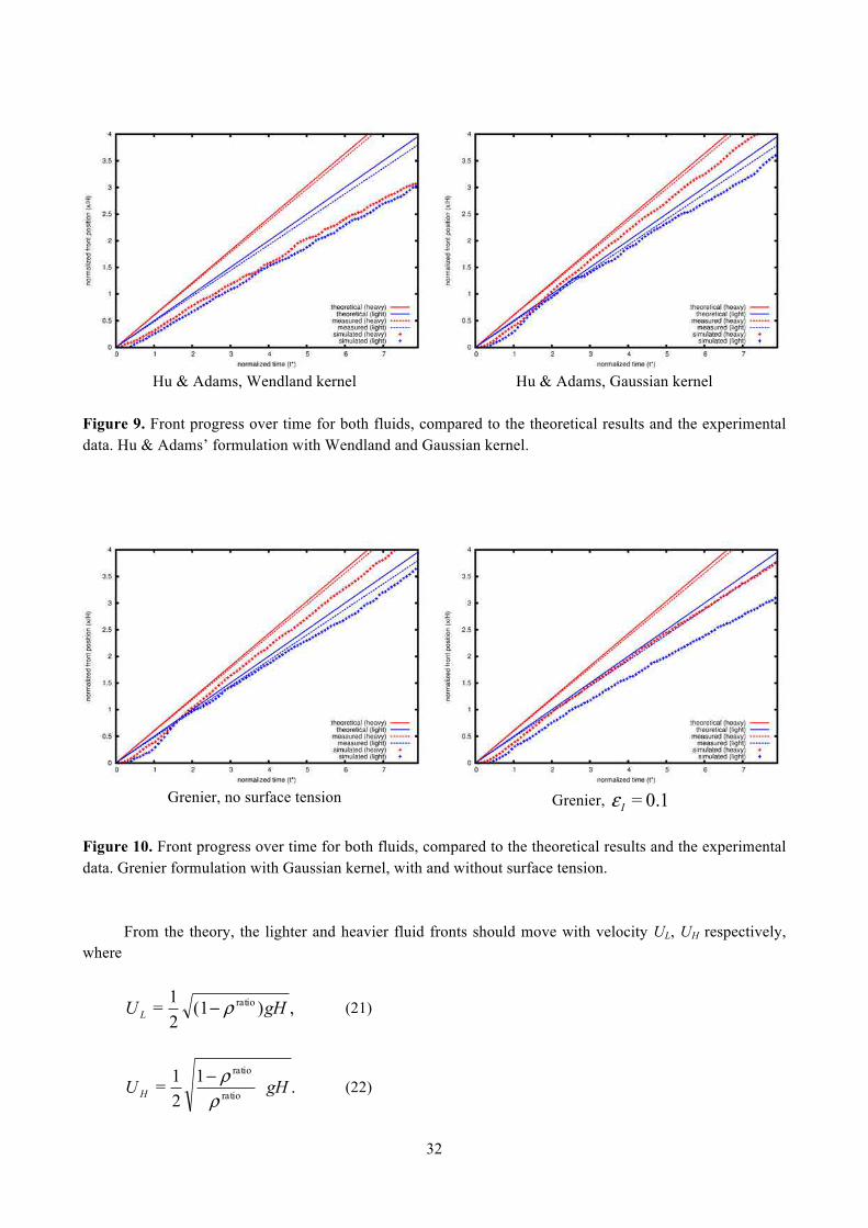
32

Hu & Adams, Wendland kernel Hu & Adams, Gaussian kernel

Figure 9. Front progress over time for both fluids, compared to the theoretical results and the experimental data. Hu & Adams’ formulation with Wendland and Gaussian kernel.

Grenier, no surface tension Grenier, 0.1=Iε

Figure 10. Front progress over time for both fluids, compared to the theoretical results and the experimental data. Grenier formulation with Gaussian kernel, with and without surface tension.

From the theory, the lighter and heavier fluid fronts should move with velocity UL, UH respectively,

where

,)(121= ratio gHUL ρ− (21)

.121= ratio

ratio

gHUH ρρ−

(22)

33

The actual measured front progress speeds for ρ ratio = 0.681 in Lowe et al.’s experiments are slightly

lower, with the measured UL being about 96% of the theoretical one, and the measured UH being about 98% of the theoretical one.

The plots in Figure 9 clearly show the influence of the kernel choice, for Hu & Adams’ formulation, whereas in Figure 10 we plot the front progress for two extremal values of the εI coefficient in the simplified surface tension model for Grenier’s formulation.

2L norm of relative error

Formulation Kernel radius, surf. tension light front heavy front

Hu & Adams Wendland/2, n.a. 10.59% 15.43%

Hu & Adams Gaussian/3, n.a. 2.087% 2.444%

Grenier Gaussian/3, 0.0=Iε 2.11% 2.447%

Grenier Gaussian/3, 0.01=Iε 2.343% 2.6%

Grenier Gaussian/3, 0.08=Iε 2.846% 2.957%

Grenier Gaussian/3, 0.1=Iε 2.892% 3.035%

Table 3. Relative error in L2 norm for our implementation over the front progress expected by the theory. Influence of formulation, kernel choice and surface tension coefficient at constant resolution Δp = 0.01m .

The relative error of the front progress of our simulations over the one predicted by the theory, for a

combination of formulations, kernel choices and values of the surface tension constant is shown in table 3. We remark that, with the exception of the case of the Wendland kernel, all configurations exhibit a small relative error (between 2% and 3%). As we shall see in the next section, this error can be further improved by running higher-resolution simulations.

34

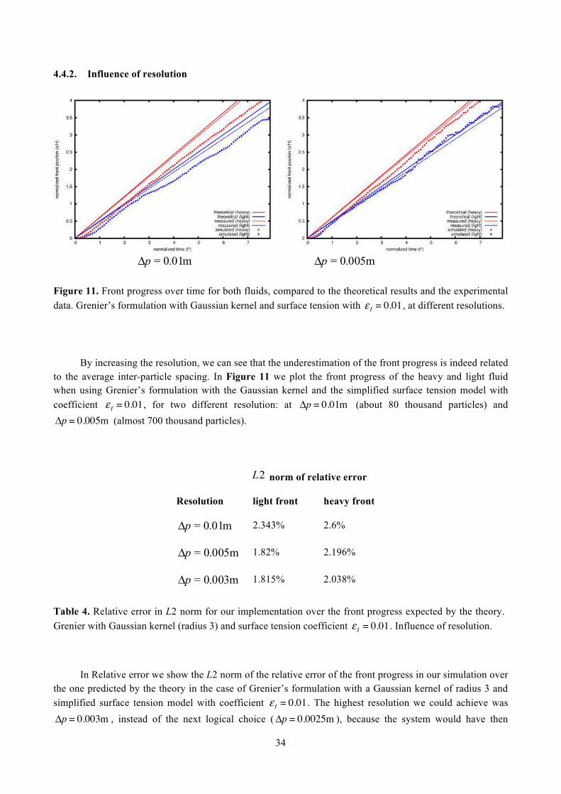
4.4.2. Influence of resolution

m0.01=pΔ m0.005=pΔ

Figure 11. Front progress over time for both fluids, compared to the theoretical results and the experimental data. Grenier’s formulation with Gaussian kernel and surface tension with ε I = 0.01 , at different resolutions.

By increasing the resolution, we can see that the underestimation of the front progress is indeed related

to the average inter-particle spacing. In Figure 11 we plot the front progress of the heavy and light fluid when using Grenier’s formulation with the Gaussian kernel and the simplified surface tension model with coefficient ε I = 0.01 , for two different resolution: at Δp = 0.01m (about 80 thousand particles) and Δp = 0.005m (almost 700 thousand particles).

2L norm of relative error

Resolution light front heavy front

m0.01=pΔ 2.343% 2.6%

m0.005=pΔ 1.82% 2.196%

m0.003=pΔ 1.815% 2.038%

Table 4. Relative error in L2 norm for our implementation over the front progress expected by the theory. Grenier with Gaussian kernel (radius 3) and surface tension coefficient ε I = 0.01 . Influence of resolution.

In Relative error we show the L2 norm of the relative error of the front progress in our simulation over

the one predicted by the theory in the case of Grenier’s formulation with a Gaussian kernel of radius 3 and simplified surface tension model with coefficient ε I = 0.01 . The highest resolution we could achieve was Δp = 0.003m , instead of the next logical choice (Δp = 0.0025m ), because the system would have then

35

required over 6 million particles, which is more than can be handled by the single-device version of GPUSPH on which our implementation is based, as discussed in section 2.1.2.

4.5. Rising bubble

4.5.1. Two-dimensional problem The rising bubble problem is essential to validate our implementation against large density differences.

While the previous validation cases presented density ratios of about an order of magnitude, the fluids present in the rising bubble problem are a liquid and air, with three orders of magnitudes in their density ratio.

R m0.025 Re 1000 ratioρ 310−

Iε 0.08

Kernel Gaussian Radius 3

Light fluid Heavy fluid

ρ ( 3m/kg ) 1 1000 γ 1.4 7 c ( s/m ) 98.055 6.933

ν ( s/m2 ) 3104.48 −⋅ 5103.5 −⋅

Table 5. Summary of parametes used in the validation of the rising bubble problem.

Again, in our set-up we follow [Grenier et al., 2009]. The air bubble has radius R (in our case, we set

R = 0.025m ), and the computational domain is a tank 6R wide and 10R tall. The Reynolds number of the

flow is Re = (2R)3g /νL =1000 and the Bond number is Bo = 4ρLgR2 /σ = 200 . The latter indicates that

effects of the surface tension σ can be neglected, allowing us to use the simplified surface tension model with a small coefficient. Following Grenier, we set ε I = 0.08 . We also use the same density and viscosity

ratios used in [Grenier et al., 2009], and thus ρL / ρG =1000 , νG /νL =128 .

The sound speeds for the two fluids are set respectively to cL =14 gR for the liquid phase and

cG =198 gR for the gaseous phase, with polytropic constants γ L = 7 and γ G =1.4 respectively. Although

the physical speed of sound in air is in fact lower than the physical speed of sound in water, in weakly compressible SPH the situation needs to be reversed, to give both fluids a similar (weak) compressibility; hence the higher speed of sound in the less dense fluid.

The parameters for the validation are summarized in Table 5.

36

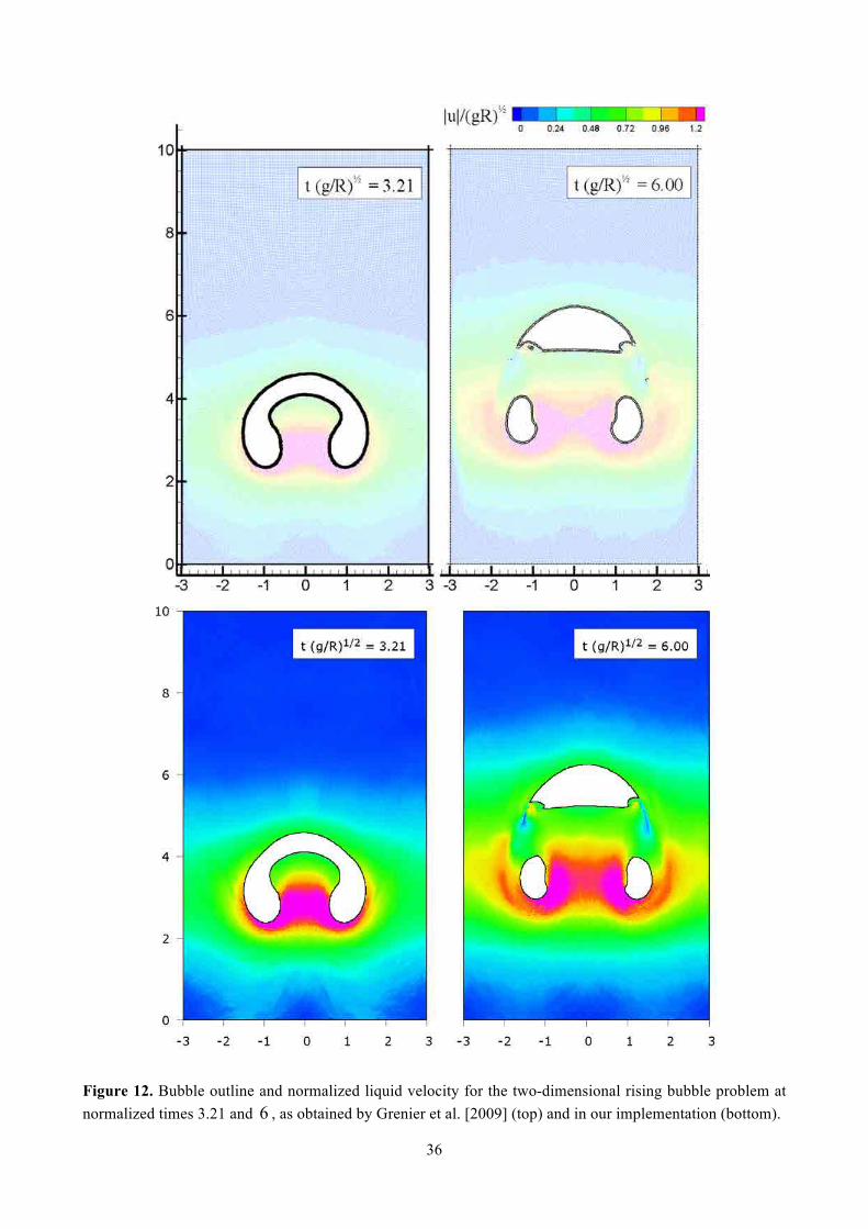
Figure 12. Bubble outline and normalized liquid velocity for the two-dimensional rising bubble problem at normalized times 3.21 and 6 , as obtained by Grenier et al. [2009] (top) and in our implementation (bottom).

37

For our tests, we used the highest resolution reported in [Grenier et al., 2009], with Δp / R = 0.025 , obtaining a system with 96,000 particles. A comparison between the results obtained by Grenier et al. and those obtained with our implementation is shown in Figure 12. The timescale is normalized with a factor t* = R / g and the velocity magnitude is normalized with a factor u* = gR .

We find that both the shape of the bubble and the velocity field are in good agreement, although some minor differences can be observed. Particularly, at normalized time 3.21 the upper surface of the bubble in our results has slightly steeper sides. As with the Rayleigh-Taylor instability, a possible explanation for these difference can be found in the unknown smoothing radius used by Grenier.

4.5.2. Influence of surface tension

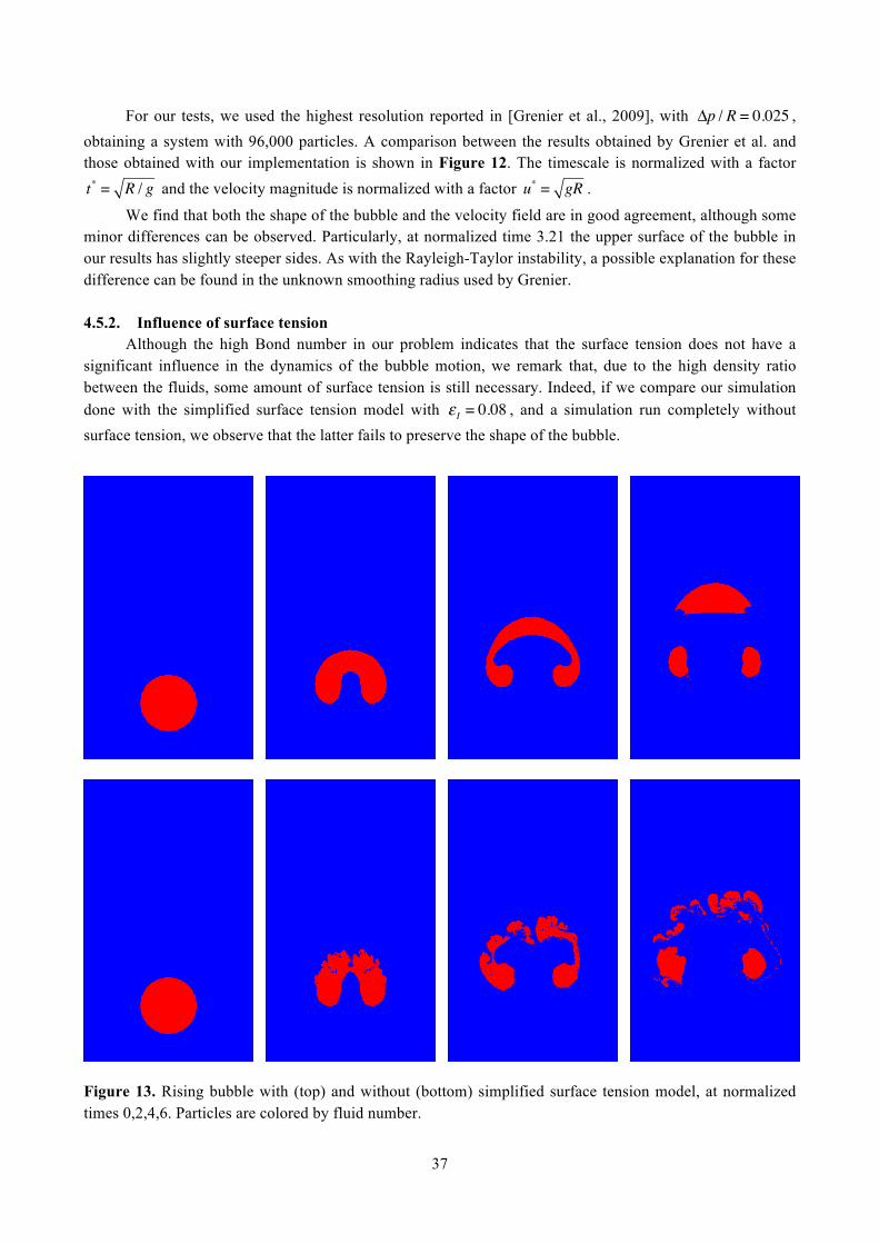
Although the high Bond number in our problem indicates that the surface tension does not have a significant influence in the dynamics of the bubble motion, we remark that, due to the high density ratio between the fluids, some amount of surface tension is still necessary. Indeed, if we compare our simulation done with the simplified surface tension model with ε I = 0.08 , and a simulation run completely without surface tension, we observe that the latter fails to preserve the shape of the bubble.

Figure 13. Rising bubble with (top) and without (bottom) simplified surface tension model, at normalized times 0,2,4,6. Particles are colored by fluid number.

38

As shown in Figure 13, the total absence of surface tension causes numerical noise developed near the interface to amplify and propagate through the bubble structure. It can be observed that despite the loss of the bubble shape, the macroscopic rising speed is still correctly preserved.

In contrast to problems with lower density ratios, such as the Rayleigh-Taylor instability or the lock exchange, the simplified surface tension model in this case is therefore necessary to preserve the shape of the bubble by smoothing out the numerical noise which is amplified by the large density difference between the two fluids.

4.5.3. Three-dimensional problem We also extended the rising bubble problem to a three-dimensional version. The domain and the fluids maintain the same properties as in the two-dimensional test just described, with the addition that the computational domain has a depth of 6R, equal to its width.

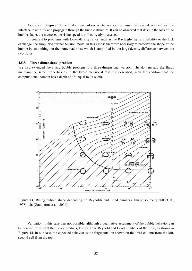
Figure 14. Rising bubble shape depending on Reynolds and Bond numbers. Image source: [Clift et al., 1978], via [Gautheron et al., 2014].

Validation in this case was not possible, although a qualitative assessment of the bubble behavior can

be derived from what the theory predicts, knowing the Reynold and Bond numbers of the flow, as shown in Figure 14. In our case, the expected behavior is the fragmentation shown on the third column from the left, second cell from the top.

39

40

Figure 15. Rising bubble in three dimensions, at normalized times 0,2,4,6. Particles are colored by their ID within the simulation. Left: view from the bottom; right: cross-section from the side.

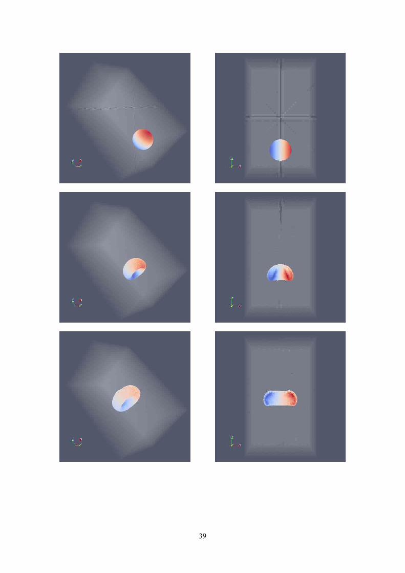
In Figure 15 we show the progress of the simulation for the three-dimensional rising bubble problem

obtained with our implementation of Grenier’s formulation, including the simplified surface tension model with ε I = 0.08 . The resolution is Δp = 2.5 ⋅10−3m , resulting in about 3 million particles, close to the maximum allowed by the single-device version of GPUSPH on which we based our implementation (see also section 2.1.2). The results qualitatively match the expected behavior, further confirming the validity of our implementation.

5. Conclusions and prospective for future work

5.1. Conclusions In the course of the project we managed to fulfill most of the requirements. In particular, completed

tasks include: • implementation of Hu & Adams’ multi-fluid SPH method; • implementation of Grenier’s multi-fluid SPH method; • validation and testing of our implementations on classic multi-fluid problems, including:

o two-dimensional Rayleigh-Taylor; o three-dimensional lock exchange / gravity current; o two-dimensional and three-dimensional rising bubble. In conclusion, we could verify the validity of our implementation both in two and three dimensions,

with density ratios as low as one order of magnitude (or less) and as high as three orders of magnitude (air water).

Our implementation was based on the open-source GPUSPH project, an implementation of SPH for CUDA-enabled GPUs. To achieve our objectives, feature such as support for two-dimensional problems and ghost-particle boundary conditions had to be included in GPUSPH.

41

5.2. Prospective for future work The most notable limitation in Hu & Adams’ and Grenier’s models is the requirement for the

realization of boundary conditions through ghost partils. An interesting prospective for future work would therefore be the extensions of these formulations (particularly Grenier’s) to allow solid boundaries to be realized with different approaches. A good candidate in this sense would be the unified semi-analytical boundary conditions from [Ferrand et al., 2013]. An implementation of Ferrand’s boundary conditions has been recently added to GPUSPH in a separate development branch [Vorobyev, 2013]. Possible future work would be the integration of this branch with the multi-fluid branch and the extension of the semi-analytical boundary condition to the multi-fluid case.

Another area where the work presented in this project could be improved concerns the implementation of the ghost-particles approach for solid boundaries. While the current implementation is correct and validated, it leaves room for optimizations that could significantly improve the performance of the code, which is currently almost an order of magnitude slower when using ghost particles compared to when using other models for the solid boundaries.

There are also a number of minor enhancements that could improve the integration between the additional features implemented for this project and the other formulations already implemented in GPUSPH. For example, the summation density is currently implemented as an option only for Hu & Adams’ formulation, but it could be extended and integrated as an option in the classical SPH formulations already featured by GPUSPH. Likewise, the simplified surface tension model which has been implemented as part of Grenier’s formulation could be extended to other formulations as well.

Finally, the work presented in this report could be integrated in the multi-GPU version of GPUSPH [Rustico et al., 2014], or in the multi-node version currently under development. This would give the possibility to run simulations at much higher resolutions than the one currently allowed on single GPUs.

Acknowledgements This report describes the work done between October 2012 and October 2013 within the framework of

the ATHOS research programme on the topic “Implementation of multi-fluid support in GPUSPH”, as defined in the cooperation contract between Électricité de France (EDF) and Istituto Nazionale di Geofisica e Vulcanologia (INGV). The work here described was performed at INGV in Catania, in the Laboratory for Technological Advance in Volcano Geophysics (TecnoLab) coordinated by Ciro Del Negro, and with the scientific supervision of Alexis Hérault (INGV), Martin Ferrand (EDF) and Damien Violeau (EDF).

References Cleary P.W. and Monaghan J.J., (1999). Conduction Modelling Using Smoothed Particle Hydrodyamics.

Journal of Computational Physics, 148(1), 227–264. Clift R., Grace J.R. and Weber M.E., (1978). Bubbles, Drops and Particles. Academic Press. Ferrand M., Laurence D.R., Rogers B.D., Violeau D., Kassiotis C., (2013). Unified semi-analytical wall

boundary conditions for inviscid, laminar or turbulent flows in the meshless SPH method. International Journal for Numerical Methods in Fluids, 71(4), 446–472.

Gautheron D., Bonnetier A., Sauvage E., Hollebecque J.-F., Brun P., Riva R., Du Terrail Y., (2014). Bubble-Stirred Metls in Vitrification. In: SYMHYDRO 2012 — New Frontiers of Simulation, Part III (P. Goubersville et al., eds.), pp. 445–455. Springer Singapore, Singapore.

42

Grenier N., Le Touzé D., Antuono M. and Colagrossi A., (2008). An improved SPH method for multi-phase simulations. In: Proceedings of the 8th International Conference on Hydrodynamics (P. Ferrant and X. B. Chen eds.). Nantes, Frances.

Grenier N., Antuono M., Le Touzé D. and Alessandrini A., (2009). An hamiltonian interface SPH formulation for multi-fluid and free surface flows. Journal of Computational Physics, 228, 8380–8393.

Grenier N., (2009) Modélisation numérique par la méthode SPH de la séparation eau-huile dans les séparateurs gravitaires. PhD thesis, École Centrale de Nantes.

Hérault A., Bilotta G. and Dalrymple R.A., (2010). SPH on GPU wih CUDA. Journal of Hyraulic Research, 48(extra issue), 74–79.

Hérault A., Bilotta G., Vicari A., Rustico E. and Del Negro C., (2011). Numerical simulation of lava flow using a GPU SPH model. Annals of Geophysics, 54(5).

Hu X. and Adams N., (2006). A multi-phase SPH method for macroscopic and mesoscopic flows. Journal of Computational Physics, 213(2), 844–861.

Lanson N. and Vila J.-P., (2008) Renormalized Meshfree Schemes I: Consistency, Stability and Hybrid methods for Conservation Laws. SIAM Journal on Numerical Analysis, 46(4), 1912–1934.

Liu G.R. and Liu M.B., (2003). Smoothed Particle Hydrodynamics: A Meshfree Particle Method. World Scientific Publishing Company.

Lowe R., Rottman J. and Linden P., (2005). The non-Boussinesq lock-exchange problem. Part 1. Theory and experiments. J. Fluid Mech., 537, 101–124.

Monaghan J.J., (1992). Smoothed Particle Hydrodynamics. Annual Review of Astronomy and Astrophysics, 30(1), 543–574.

Monaghan J.J., (2005). Smoothed Particle Hydrodynamics. Reports on Progress in Physics, 68(8), 1703. Monaghan J.J. and Kajtar J.B., (2009). SPH particle boundary forces for arbitrary boundaries. Computer

Physics Communications, 180(10), 1811–1820. Monaghan J.J and Rafiee A., (2012). A simple SPH algoithm for multi-fluid flow with high density ratios.

International Journal for Numerical Methods in Fluids, 71(5), 537–561. Morris J.P., Fox P.J. and Zhu Y., (1997). Modeling low Reynolds number incompressible flows usin SPH.

Journal of Computational Physics, 136(1), 214–226. Rustico E., Bilotta G., Hérault A., Del Negro C. and Gallo G., (2014). Advances in multi-GPU Smoothed

Particle Hydrodynamics simulations. IEEE Transactions on Parallel and Distributed Systems, 25(1), 43–52.

Shepard D., (1968). A two-dimensional interpolation function for irregularly spaced data. In: ACM ’68 Proceedings of the 1968 23rd ACM national confernce, 517–524.

Vorobyev A., (2013). Implementing unified semi-analytical wall boundary conditions in GPU-SPH. Post-doctoral report.

Wendland H., (1995). Piecewise polynomial, positive definite and compactly supported radial functions of minimal degree. Advances in Computational Mathematics, 4(1), 389–396.

ISSN 1590-2595

ISSN 2039-7941

I Quaderni di Geofisica coprono tutti i campi disciplinari sviluppati all'interno dell'INGV,dando particolare risalto alla pubblicazione di dati, misure, osservazioni e loro elaborazionianche preliminari, che per tipologia e dettaglio necessitano di una rapida diffusione nellacomunità scientifica nazionale ed internazionale. La pubblicazione on-line fornisce accessoimmediato a tutti i possibili utenti. L’Editorial Board multidisciplinare garantisce i requisitidi qualità per la pubblicazione dei contributi.

ISSN 2039-6651

La collana Miscellanea INGV nasce con l'intento di favorire la pubblicazione di contributiscientif ici riguardanti le attività svolte dall'INGV (sismologia, vulcanologia, geologia,geomagnetismo, geochimica, aeronomia e innovazione tecnologica). In particolare, lacollana Miscellanea INGV raccoglie reports di progetti scientifici, proceedings di convegni,manuali, monografie di rilevante interesse, raccolte di articoli ecc..

I Rapporti Tecnici INGV pubblicano contributi, sia in italiano che in inglese, di tipo tecnologicoe di rilevante interesse tecnico-scientifico per gli ambiti disciplinari propri dell'INGV. Lacollana Rapporti Tecnici INGV pubblica esclusivamente on-line per garantire agli autori rapiditàdi diffusione e agli utenti accesso immediato ai dati pubblicati. L’Editorial Boardmultidisciplinare garantisce i requisiti di qualità per la pubblicazione dei contributi.

Quaderni di

apportitecnici

miscellaneaINGV

http://istituto.ingv.it/l-ingv/produzione-scientifica/quaderni-di-geofisica/

http://istituto.ingv.it/l-ingv/produzione-scientifica/rapporti-tecnici-ingv/

http://istituto.ingv.it/l-ingv/produzione-scientifica/miscellanea-ingv/

Coordinamento editoriale e impaginazioneCentro Editoriale Nazionale | INGV

Progetto grafico e redazionaleDaniela Riposati | Laboratorio Grafica e Immagini | INGV

© 2014 INGV Istituto Nazionale di Geofisica e VulcanologiaVia di Vigna Murata, 605

00143 RomaTel. +39 06518601 Fax +39 065041181

http://www.ingv.it

Istituto Nazionale di Geofisica e Vulcanologia