PSZ 19:16 (Pind. 1/97)
UNIVERSITI TEKNOLOGI MALAYSIA
BORANG PENGESAHAN STATUS TESIS JUDUL: DIRECT TORQUE CONTROL OF INDUCTION MOTOR DRIVES USING SPACE VECTOR MODULATION (DTC - SVM)
SESI PENGAJIAN: 2004/2005
Saya ZOOL HILMI BIN ISMAIL (HURUF BESAR)
mengaku membenarkan tesis (PSM/Sarjana/Doktor Falsafah)* ini disimpan di Perpustakaan Universiti Teknologi Malaysia dengan syarat-syarat kegunaan seperti berikut:
1. Tesis adalah hakmilik Universiti Teknologi Malaysia. 2. Perpustakaan Universiti Teknologi Malaysia dibenarkan membuat salinan untuk tujuan
pengajian sahaja. 3. Perpustakaan dibenarkan membuat salinan tesis ini sebagai bahan pertukaran antara institusi
pengajian tinggi. 4. **Sila tandakan ( )
SULIT
(Mengandungi maklumat yang berdarjah keselamatan atau kepentingan Malaysia seperti yang termaktub di dalam AKTA RAHSIA RASMI 1972)
TERHAD
(Mengandungi maklumat TERHAD yang telah ditentukan oleh organisasi/badan di mana penyelidikan dijalankan)
TIDAK TERHAD
Disahkan oleh
(TANDATANGAN PENULIS) (TANDATANGAN PENYELIA)
Alamat Tetap:
Lot 316, Kampung Kubang Tin, Jln. Aril, Dr. Nik Rumzi Nik Idris
Melor, 16400 Kota Bharu, Kelantan. Nama Penyelia
Tarikh: 11 November 2005 Tarikh: 11 November 2005
CATATAN: * Potong yang tidak berkenaan. ** Jika tesis ini SULIT atau TERHAD, sila lampirkan surat dari pihak berkuasa /
organisasi berkenaan dengan menyatakan sekali sebab dan tempoh tesis ini perlu dikelaskan sebagai SULIT atau TERHAD.
Tesis dimaksudkan sebagai tesis bagi Ijazah Doktor Falsafah dan Sarjana secara penyelidikan, atau disertasi bagi pengajian secara kerja kursus dan penyelidikan, atau Laporan Projek Sarjana Muda (PSM).

I hereby declare that I have read this thesis and in my opinion this thesis is sufficient
in term of scope and quality for the award of the degree of Master of Engineering
(Electrical - Mechatronics and Automatic Control).
Signature :
Name : Dr. Nik Rumzi Nik Idris.
Date : 11 November 2005
DIRECT TORQUE CONTROL OF INDUCTION MOTOR DRIVES USING
SPACE VECTOR MODULATION (DTC-SVM)
ZOOL HILMI ISMAIL
A project report submitted in partial fulfillment
of the requirement for the award of the degree of
Master of Engineering
(Electrical - Mechatronics & Automatic Control)
Faculty of Electrical Engineering
Universiti Teknologi Malaysia
NOVEMBER, 2005
ii
I declare that this thesis entitled “Direct Torque Control of Induction Motor
Drives Using Space Vector Modulation (DTC-SVM)” is the result of my own work
and the materials which are not the results of my own work have been clearly
acknowledged.
Signature :
Name : Zool Hilmi Ismail
Date : 11 November 2005

iii
Specially dedicated from ‘Abe Long’ to
my beloved mother, father, brother, sister and a special friend who have
encouraged, guided and inspired me throughout my journey of education

iv
ACKNOWLEDGEMENT
I would like to take this opportunity to express my deepest gratitude to my
project supervisor, Dr. Nik Rumzi Nik Idris who has persistently and determinedly
assisted me during the whole course of this project. It would have been very difficult
to complete this project without the enthusiastic support, insight and advice given by
him.
My outmost thank also goes to my family who has given me support
throughout my academic years. Without them, I might not be the person I am today.
My special gratitude to Arias Pujol, as his thesis has been my guidance and
giving some ideas to support my project. It is of my greatest thanks and joy that I
have met these people. Thank you.
v
ABSTRACT
Direct Torque Control is a control technique used in AC drive systems to
obtain high performance torque control. The conventional DTC drive contains a pair
of hysteresis comparators, a flux and torque estimator and a voltage vector selection
table. The torque and flux are controlled simultaneously by applying suitable voltage
vectors, and by limiting these quantities within their hysteresis bands, de-coupled
control of torque and flux can be achieved. However, as with other hysteresis-bases
systems, DTC drives utilizing hysteresis comparators suffer from high torque ripple
and variable switching frequency. The most common solution to this problem is to
use the space vector depends on the reference torque and flux. The reference voltage
vector is then realized using a voltage vector modulator. Several variations of
DTC-SVM have been proposed and discussed in the literature. The work of this
project is to study, evaluate and compare the various techniques of the DTC-SVM
applied to the induction machines through simulations. The simulations were carried
out using MATLAB/SIMULINK simulation package. Evaluation was made based on
the drive performance, which includes dynamic torque and flux responses, feasibility
and the complexity of the systems.
vi
ABSTRAK
Sistem kawalan tenaga putaran secara terus adalah teknik kawalan yang
digunakan dalam pemacu sistem arus ulang-alik dimana ia bertujuan mencapai
kawalan tenaga putaran yang lebih baik. Sistem kawalan yang ada sekarang ini
terdiri daripada pembanding histeresis, penafsiran fluks dan tenaga putaran dan juga
jadual pemilihan vektor voltan. Fluks dan tenaga putaran dapat dikawal secara
serentak dengan mengenakan vektor voltan yang sesuai dan menghadkan
kuantiti-kuantiti ini dalam batasan yang telah ditetapkan, maka kawalan tenaga
putaran dan fluks secara berasingan dapat dicapai. Walaubagaimanapun, pengunaan
pembanding histeresis boleh menghasilkan riak tenaga putaran yang tinggi di
samping perubahan yang tidak menentu dalam frekuensi pensuisan. Biasanya,
penyelesaian untuk masalah ini adalah dengan menggunakan ruangan vektor (space
vector) yang bergantung kepada fluks dan tenaga putaran. Voltan rujukan
kemudiannya direalisasikan menggunakan pemodulat vektor voltan. Beberapa
kaedah DTC-SVM telah dicadangkan dan dibincangkan dan pelaksanaan tugas untuk
projek ini adalah untuk mengkaji, menilai dan membuat perbandingan secara
simulasi bagi beberapa teknik DTC-SVM yang diaplikasikan terhadap motor
induktor. Simulasi dijalankan dengan menggunakan pakej MATLAB/SIMULINK.
Penilaian dibuat berdasarkan perihal prestasi pemacu yang mana terdiri daripada
dinamik untuk tenaga putaran, kebolehlaksaan, dan kerumitan dalam sistem.

vii
TABLE OF CONTENTS
CHAPTER TITLE PAGE
TITLE i
DECLARATION ii
DEDICATION iii
ACKNOWLEDGEMENT iv
ABSTRACT v
ABSTRAK vi
TABLE OF CONTENTS vii
LIST OF TABLES xi
LIST OF FIGURES xii
LIST OF SYMBOLS xvi
LIST OF APPENDICES xx
1 INTRODUCTION
1.1 Overview of Induction Motor 1
1.2 Aim of the Research Project 5
1.3 Scope of Work Project 6
viii
1.4 Thesis Outline 7
2 INDUCTION MOTOR MODEL
2.1 Equation of Induction Motor Model 9
2.1.1 Voltage Equations 11
2.1.2 Applying Park’s Transform 13
2.1.3 Voltage Matrix Equations 15
2.2 Space Phasor Notation 16
2.2.1 Current Space Phasors 18
2.2.2 Flux Linkage Space Phasors 21
2.2.3 The Space Phasors of Stator and Rotor Voltages 27
2.2.4 Space Phasor Form of the Motor Equations 28
2.3 Torque Expressions
2.3.1 Introduction 34
2.3.2 Deduction of the Torque Expression by
Mean of Energy Considerations 35
3 DIRECT TORQUE CONTROL: PRINCIPLES
AND GENERALITIES
3.1 Induction Motor Controllers
3.1.1 Voltage /Frequency 37
3.1.2 Vector Control 38
3.1.3 Field Acceleration method 39
3.1.4 Direct Torque Control 39
3.2 Principles of Direct Torque Control
3.2.1 Introduction 40
ix
3.2.2 DTC Controller 42
3.2.3 DTC Schematic 45
3.2.4 Parameter Detuning Affects 50
4 DIRECT TORQUE CONTROL –
SPACE VECTOR MODULATION (DTC – SVM)
4.1 Introduction 51
4.2 Various Direct Torque Control–Space Vector Modulations
(DTC-SVM)
4.2.1 DTC-SVM with Closed-Loop Torque Control 53
4.2.2 DTC-SVM with Closed-Loop Flux Control 59
4.2.3 DTC-SVM with Closed-Loop Torque and Flux
Control Operating in Cartesian Coordinates 64
5 ANALYSIS AND COMPARISON
5.1 Introduction 71
5.2 Simulink Model
5.2.1 Equation Used in Model 72
5.2.2 Conventional Direct Torque Control 74
5.2.3 DTC-SVM with Closed-Loop Torque Control 76
5.2.4 DTC-SVM with Closed-Loop Flux Control 77
5.2.5 DTC-SVM with Closed-Loop Torque and Flux
Control Operating in Cartesian Coordinates 79
5.3 Simulated Results 80
5.4 Interim Conclusions 87

x
6 CONCLUSION AND RECOMMENDATION FOR
FUTURE WORK
6.1 Conclusion 92
6.2 Recommendation for Future Work 94
REFERENCES 96
xi
LIST OF TABLES
TABLE NO. TITLE PAGE
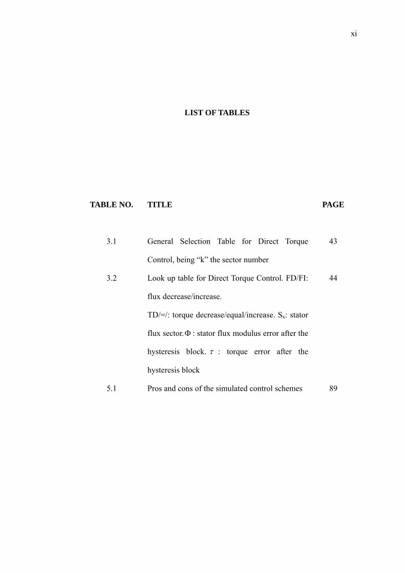
3.1 General Selection Table for Direct Torque
Control, being “k” the sector number
43
3.2 Look up table for Direct Torque Control. FD/FI:
flux decrease/increase.
TD/=/: torque decrease/equal/increase. Sx: stator
flux sector.Φ : stator flux modulus error after the
hysteresis block. τ : torque error after the
hysteresis block
44
5.1 Pros and cons of the simulated control schemes 89
xii
LIST OF FIGURES
FIGURE NO. TITLE PAGE
1.1 Overview of induction motor control methods 4
2.1 Cross-section of an elementary symmetrical
three-phase machine
10
2.2 Equivalence physics transformation 13
2.3 Cross-section of an elementary symmetrical
three-phase machine, with two different frames,
the D-Q axis which represent the stationary
frame fixed to the stator, and α-β axis which
represent rotating frame fixed to the rotor
18
2.4 Stator-current space phasor expressed in
accordance with the rotational frame fixed to the
rotor and the stationary frame fixed to the stator
26
2.5 A magnitude represented by means of the vector,
and its angle referred to the three different axes.
The three different axis are: sD-sQ fixed to the
28
xiii
stator, rα-rβ fixed to the rotor whose speed is wm
and finally the general reference frame
represented by means of the axis x-y whose
speed is equal to wg
3.1 Stator flux vector locus and different possible
switching voltage vectors.
FD: flux decrease. FI : flux increase. TD: torque
decrease. TI: torque increase
43
3.2 Direct Torque Control Schematic 46
4.1 Reference and estimated flux relations 55
4.2 Block scheme of DTC-SVM with closed-loop
torque control
56
4.3 Rotor flux estimator block diagram 58
4.4 Block scheme of DTC-SVM with closed-loop
flux control
60
4.5 Block diagram to determine the reference value
of the stator flux vector
61
4.6 Stator flux components in synchronous reference
frame
62
4.7 Stator flux estimator block diagram 63
4.8 Rotor flux estimator block diagram 64
4.9 Schematic of the stator-flux-oriented control of
an induction machine with a space vector PWM
inverter
65

xiv
4.10 Stator magnetizing-current space phasor and
rotor-current space phasor
68
4.11 Stator flux estimator block diagram 69
5.1 Conventional Direct Torque Control Schematic
using SIMULINK/MATLAB
75
5.2 DTC-SVM scheme with closed-loop torque
control schematic using SIMULINK/MATLAB
77
5.3 DTC-SVM scheme with closed-loop flux control
schematic using SIMULINK/MATLAB
78
5.4 DTC-SVM scheme with closed-loop torque and
flux control operating in Cartesian
coordinates-stator flux-oriented control
schematic using SIMULINK/MATLAB
80
5.5 Dynamic response for conventional DTC 81
5.6 Dynamic response for DTC-SVM with
closed-loop torque control
82
5.7 Dynamic response for DTC-SVM scheme with
closed-loop flux control
82
5.8 Dynamic response for stator field oriented
control
83
5.9 Torque response for conventional DTC 84
5.10 Torque response for DTC-SVM scheme with
closed-loop torque
84
5.11 Torque response for DTC-SVM scheme with
closed-loop flux control
85
xv
5.12 Torque response for stator field oriented control 85
5.13 Stator flux path in d-q plane for conventional
DTC
86
5.14 Stator flux path in d-q for DTC-SVM scheme
with closed-loop torque
86
5.15 Stator flux path in d-q for stator field oriented
control
87
xvi
LIST OF SYMBOLS
a - 120° operator.
rii (t) - Rotor current per phase.
ir - Space phasor of the rotor current expressed in the rotor
reference frame.
i 'r - Space phasor of the rotor current expressed in the stator
reference frame.
sii (t) - Stator current per phase.
is - Space phasor of the stator current expressed in the
stator reference frame.
i 's - Space phasor of the stator current expressed in the rotor
reference frame.
mL - Three phase magnetizing inductance.
rL - Total three phase rotor inductance.
rL - Rotor self-inductance.
r1L - Leakage rotor inductance.
rmL - Rotor magnetizing inductance.
sL - Total three phase stator inductance.
xvii
sL - Stator self-inductance.
smL - Stator magnetizing inductance.
s1L - Leakage stator inductance.
rM - Mutual inductance between rotor windings.
sM - Mutual inductance between stator windings.
srM - Maximal value of the stator-rotor mutual inductance.
p - Derivation operator.
P - Pair of poles.
rR - Rotor resistance.
sR - Stator resistance.
s - Slip.
1/s - Integrator operator.
Te - Instantaneous value of the electromagnetic torque.
pcT - Instant torque referred to the nominal torque and in
percentage.
Ts=Tz - Sampling time.
riu (t) - Rotor voltage per phase.
ru - Space phasor of the rotor voltage expressed in the rotor
reference frame.
ru ' - Space phasor of the rotor voltage expressed in the stator
reference frame.
siu (t) - Stator voltage per phase.
su - Space phasor of the stator voltage expressed in the
stator reference frame.
xviii
su ' - Space phasor of the stator voltage expressed in the rotor
reference frame.
mω - Mechanical speed
gω - General speed
rω - Rotor pulsation
sω - Stator pulsation
ρr - Phase angle of the rotor flux linkage space phasor with
respect to the direct-axis of the stator reference frame.
ρs - Phase angle of the stator flux linkage space phasor with
respect to the direct-axis of the stator reference frame.
θm - Stator to rotor angle.
θr - Rotor angle.
θs - Stator angle.
riψ (t) - Flux linkage per rotor winding.
rψ - Space phasor of the rotor flux linkage expressed in the
rotor reference frame.
rψ ' - Space phasor of the rotor flux linkage expressed in the
stator reference frame.
siψ (t) - Flux linkage per stator winding.
sψ - Space phasor of the stator flux linkage expressed in the
stator reference frame.
sψ ' - Space phasor of the stator flux linkage expressed in the
rotor reference frame.
α/β - Direct- and quadrature-axis components in the rotor
reference frame.
xix
d/q - Rotor direct- and quadrature-axis components in the
stator reference frame.
D/Q - Stator direct- and quadrature-axis components in the
stator reference frame.
g - General reference frame.
m - Magnetizing.
r - Rotor
ra,rb,rc - Rotor phases.
Ref - Reference.
s - Stator.
sA,sB,sC - Stator phases.
x/y - Direct- and quadrature-axis components in general
reference frame or in special reference frames.
x - Cross vector product.
* - Complex conjugate.

xx
LIST OF APPENDICES
APPENDICES TITLE PAGE
A Matlab Function of Induction Motor Model 101
B Voltage Vector Selection Table in Matlab file 106
1
CHAPTER 1
INTRODUCTION
1.1 OVERVIEW OF INDUCTION MOTOR
The induction motors have more advantages over the rest of motors. The
main advantage is that induction motors do not require an electrical connection
between the stationary and the rotating parts of the motor. Therefore, they do not
need any mechanical commutator (brushes), leading to the fact that they are
maintenance free motors.
Besides, induction motors also have low weight and inertia, high efficiency
and a high overload capability. Therefore, they are cheaper and more robust, and less
proves to any failure at high speeds. Furthermore, the motor can work in explosive
2
environments because no sparks are produced.
Taking into account all of the advantages outlined above, the induction
motors must be considered as the perfect electrical to mechanical energy converter.
However, mechanical energy is more than often required at variable speeds, where
the speed control system is not an insignificant matter.
The only effective way of producing an infinitely variable induction motor
speed drive is to supply the induction motor with three phase voltages of variable
frequency and variable amplitude. A variable frequency is requires because the rotor
speed depends on the speed of the rotating magnetic field provided by the stator. A
variable voltage is required because the motor impedance reduces at the low
frequencies and consequently the current has to be limited by means of reducing the
supply voltages.[1][2]
Induction motors are also available with more than three stator windings to
allow a change of the number of pole pairs. However, a motor with several windings
is more expensive because more than three connections to the motor are needed and
only certain discrete speeds are available.
Another alternative method of speed control can be realized by means of a
wound rotor induction motor, where the rotor winding ends are brought out to slip
3
rings. However, this method obviously removes most of the advantages of the
induction motors and it also introduces additional losses. By connecting resistors or
reactance in series with the stator windings of the induction motors, poor
performance is achieved.[2][33]
Historically, several general controllers have been developed:
Scalar controllers: Despite the fact that “Voltage-Frequency” (V/f) is simplest
controller, it is the most widespread, being in the majority of the industrial
applications. It is known as a scalar control and acts by imposing a constant
relation between voltage and frequency. The structure is simple and it is normally
used without speed feedback. However, this controller does not achieve a good
accuracy in both speed and torque responses, mainly regarding to the fact that the
stator flux and torque are not directly controlled. Even though, as long as the
parameters are identified, the accuracy in the speed can be 2% (except in a very
low speed), and the dynamic response can be approximately around 50ms.[3][4]
Vector Controllers: In these types of controller, there are control loops for
controlling both the torque and the flux.[5] The most widespread controllers of
this type are the ones that use vector transform such as either Park or Ku. Its
accuracy can reach values such as 0.5% regarding the speed and 2% regarding
the torque, even when at stand still. The main disadvantages are the huge
computational capability required and the compulsory good identification of the
motor parameters.[6]
4
Field Acceleration Method: This method is based on the maintaining the
amplitude and the phase of the stator current constant, whilst avoiding
electromagnetic transients. Therefore, the equations can be simplified saving the
vector transformation, which occurs in the vector controllers. This technique has
achieved some computation reduction, thus overcoming the main problem with
vector controllers and allowing this method to become an important alternative to
vector controllers.[8][10]
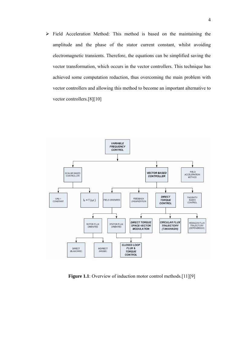
Figure 1.1: Overview of induction motor control methods.[11][9]
5
Direct torque control (DTC) has emerged over the last decade to become one
possible alternative to the well-known Vector Control of Induction Machines. Its
main characteristic is the good performance, obtaining results as good as the classical
vector control but with several advantages based on its simpler structure and control
diagram.[7]
DTC is said to be one of the future ways of controlling the induction machine
in four quadrants.[1][11] In the DTC, it is possible to control directly the stator flux
and the torque by selecting the appropriate inverter state. This method still required
further research in order to improve the motor’s performance, as well as achieve a
better behavior regarding environment compatibility (Electro Magnetic Interference
and Energy), that is desired nowadays for all industrial applications.
1.2 AIM OF THE RESEARCH PROJECT
The main objective of this project is to study on the various techniques of
direct torque control (DTC) based on Space Vector Modulation (DTC-SVM) applied
to induction motor drive systems. With DTC-SVM, it is possible to achieve fixed
switching frequency and low torque ripple, hence overcoming the major drawbacks
of conventional DTC. This project will simulate and perform analysis on some of the
present DTC-SVM drives using MATLAB/SIMULINK simulation package.
6
The conventional DTC is firstly analyzed and proved by means of
MATLAB/SIMULINK simulation. Then, the various technique of direct torque
control based on Space Vector Modulation will be presented and also the pros and
cons of the present DTC-SVM control strategies will be highlighted.
1.3 SCOPE OF WORK PROJECT
The project is divided into three stages. This is to ensure that the project is
conducted within its intended boundary and is heading to the right direction to
achieve it objectives:
The first stage is to study on the working principle of the direct torque control
of induction motor drive that utilizes hysteresis comparators and to
understand on the limitations of this conventional control technique.
Secondly, it will concentrate on performing the simulations on the various
types of DTC-SVM for induction motor drive systems.
The third stage of the project is to analyze on the performance of the various
control techniques of DTC-SVM based on the MATLAB/SIMULINK
simulation results.
7
1.4 THESIS OUTLINE
This section will give an outlines of the structure of the thesis. The following
is an explanation for each chapter.
Chapter 2 discusses a mathematical model of cage rotor induction motors.
Different ways of implementing these models are presented. The elements of space
phasor notation are also introduced and used to develop a compact notation. Then, all
the model equations will be applied on the further chapter.
Chapter 3 is devoted to introduce different Direct Torque Control (DTC)
strategies. This chapter summarizes different induction motor controllers, such as the
very well known vector control and “V/Hz”. The principles of DTC are thoroughly
discussed and presented.
Chapter 4 deals with different kinds of Direct Torque Control with Space
Vector Modulation (DTC-SVM) control techniques. All the basic principles and
detail derivation of voltage reference for each control schemes are discussed within
this chapter. Actually, the comparison between each control algorithm already can be
observed on this chapter.

8
Chapter 5 gives the analysis and states the differences between conventional
DTC, DTC-SVM with torque control, DTC-SVM with flux loop control and
DTC-SVM with torque and flux loop control in term of torque response, control
technique, stator flux trajectory and etc.
Chapter 6 presents the conclusions and recommendation for future works.
Finally, all C-programming used in the simulations are listed in the appendixes.
9
CHAPTER 2
INDUCTION MOTOR MODEL
2.1 EQUATION OF THE INDUCTION MOTOR MODEL
A dynamic model of the machine subjected to control must be known in order
to understand and design vector controlled drives. Due to the fact that every good
control has to face any possible change of the plant, it could be said that the dynamic
model of the machine could be just a good approximation of the real plant.
Nevertheless, the model should incorporate all the important dynamic effects
occurring during both steady state and transient operations. Furthermore, it should be
valid for any changes in the inverter’s supply such as voltages or currents.[6]
Such a model can be obtained by means of either the space vector phasor
10
theory or two-axis theory of electrical machines. Despite the compactness and the
simplicity of the space phasor theory, both methods are actually close and both
methods will be explained.
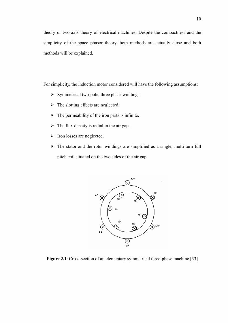
For simplicity, the induction motor considered will have the following assumptions:
Symmetrical two-pole, three phase windings.
The slotting effects are neglected.
The permeability of the iron parts is infinite.
The flux density is radial in the air gap.
Iron losses are neglected.
The stator and the rotor windings are simplified as a single, multi-turn full
pitch coil situated on the two sides of the air gap.
Figure 2.1: Cross-section of an elementary symmetrical three-phase machine.[33]
11
2.1.1 VOLTAGE EQUATIONS
The stator voltages will be formulated in this section from the motor natural
frame, which is the stationary reference frame fixed to the stator. In a similar way,
the rotor voltages will be formulated to the rotating frame fixed to the rotor.
In the stationary reference frame, the equations can be expressed as follows:
sAsA s sA
dΨ (t)u (t)=R i (t)+dt
(2.1)
sBsB s sB
dΨ (t)u (t)=R i (t)+dt
(2.2)
sCsC s sC
dΨ (t)u (t)=R i (t)+dt
(2.3)
Similar way expressions can be obtained for the rotor:
rara r ra
dΨ (t)u (t)=R i (t)+dt
(2.4)
rbrb r rb
dΨ (t)u (t)=R i (t)+dt
(2.5)
rcrc r rc
dΨ (t)u (t)=R i (t)+dt
(2.6)
The instantaneous stator flux linkage values per phase can be expressed as:
sA s sA s sB s sC sr m ra sr m rb sr m rcΨ =L i +M i +M i +M cosθ i +M cos(θ +2π/3)i +M cos(θ +4π/3)i
(2.7)
12
sB s sB s sA s sC sr m rb sr m rc sr m raΨ =L i +M i +M i +M cosθ i +M cos(θ +2π/3)i +M cos(θ +4π/3)i
(2.8)
sC s sC s sA s sB sr m rc sr m ra sr m rbΨ =L i +M i +M i +M cosθ i +M cos(θ +2π/3)i +M cos(θ +4π/3)i
(2.9)
In a similar way’ the rotor flux linkages can be expressed as follows:
ra r ra r rb r rc sr m sA sr m sB sr m sCΨ =L i +M i +M i +M cos(-θ )i +M cos(-θ +2π/3)i +M cos(-θ +4π/3)i
(2.10)
rb r rb r ra r rc sr m sB sr m sC sr m sAΨ =L i +M i +M i +M cos(-θ )i +M cos(-θ +2π/3)i +M cos(-θ +4π/3)i
(2.11)
rc r rc r ra r rb sr m sC sr m sA sr m sBΨ =L i +M i +M i +M cos(-θ )i +M cos(-θ +2π/3)i +M cos(-θ +4π/3)i
(2.12)
Taking into account all the previous equations, and using the matrix notation in order
to compact all the expressions, the following expression is obtained:
s s s sr sr srs m m1 m2sA
s s s sr sr srs m2 msB
s s s sr sr srsC s m1 m2
sr sr sr s sra m m1 m2 s
rb
rc
R +pL pM pM pM cosθ pM cosθ pM cosθupM R +pL pM pM cosθ pM cosθ pM cosθu
u pM pM R +pL pM cosθ pM cosθ pM cosθ=
u pM cosθ pM cosθ pM cosθ R +pL pMuu
⎡ ⎤⎢ ⎥⎢ ⎥⎢ ⎥⎢ ⎥⎢ ⎥⎢ ⎥⎢ ⎥⎢ ⎥⎣ ⎦
m1
m
sA
sB
sC
s ra
rbsr sr sr s s sm2 m m1 s
rcsr sr sr s s sm1 m2 m s
iiiipMipM cosθ pM cosθ pM cosθ pM R +pL pMipM cosθ pM cosθ pM cosθ pM pM R +pL
⎡ ⎤ ⎡ ⎤⎢ ⎥ ⎢ ⎥⎢ ⎥ ⎢ ⎥⎢ ⎥ ⎢ ⎥⎢ ⎥ ⎢ ⎥⎢ ⎥ ⎢ ⎥⎢ ⎥ ⎢ ⎥⎢ ⎥ ⎢ ⎥⎢ ⎥ ⎢ ⎥⎣ ⎦⎢ ⎥⎣ ⎦
(2.13)
13
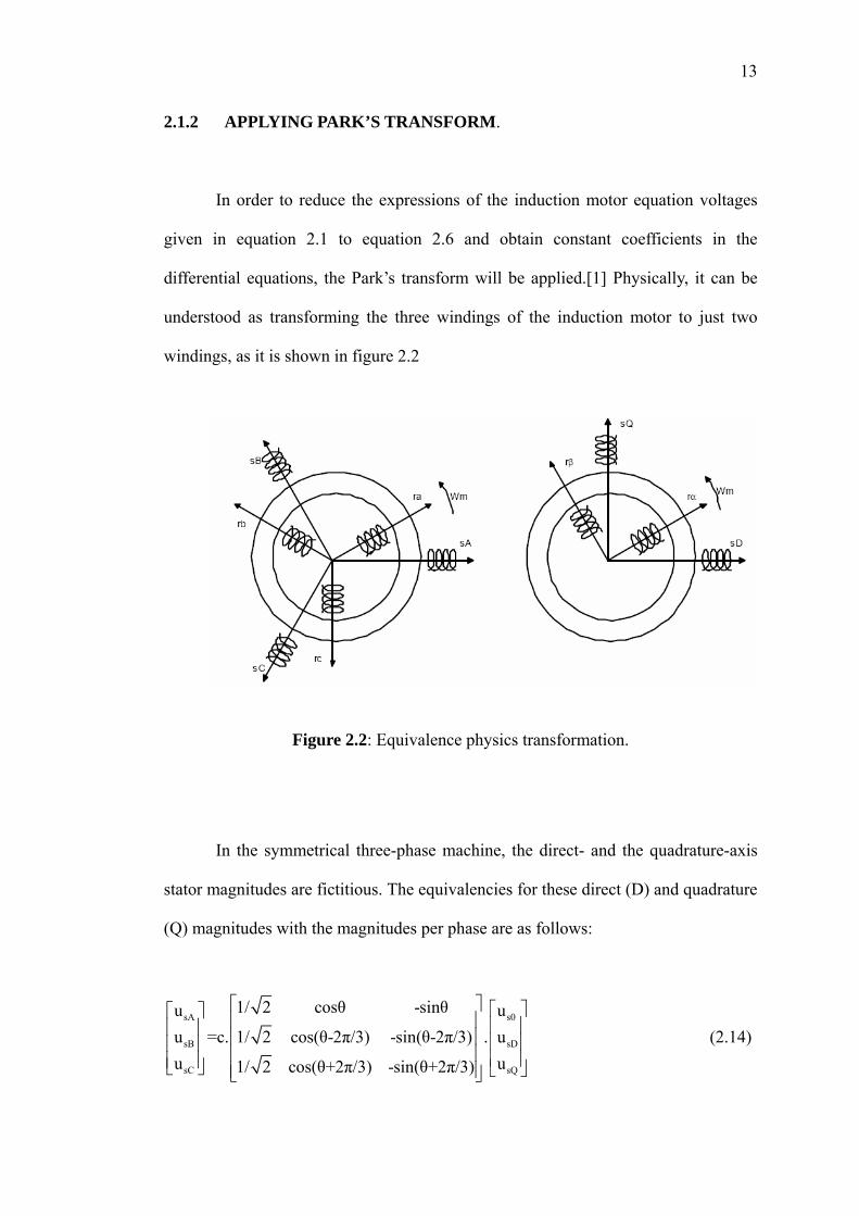
2.1.2 APPLYING PARK’S TRANSFORM.
In order to reduce the expressions of the induction motor equation voltages
given in equation 2.1 to equation 2.6 and obtain constant coefficients in the
differential equations, the Park’s transform will be applied.[1] Physically, it can be
understood as transforming the three windings of the induction motor to just two
windings, as it is shown in figure 2.2
Figure 2.2: Equivalence physics transformation.
In the symmetrical three-phase machine, the direct- and the quadrature-axis
stator magnitudes are fictitious. The equivalencies for these direct (D) and quadrature
(Q) magnitudes with the magnitudes per phase are as follows:
sA s0
sB sD
sC sQ
1/ 2 cosθ -sinθu uu =c. 1/ 2 cos(θ-2π/3) -sin(θ-2π/3) . uu u1/ 2 cos(θ+2π/3) -sin(θ+2π/3)
⎡ ⎤ ⎡ ⎤⎡ ⎤ ⎢ ⎥ ⎢ ⎥⎢ ⎥ ⎢ ⎥ ⎢ ⎥⎢ ⎥ ⎢ ⎥ ⎢ ⎥⎢ ⎥⎣ ⎦ ⎣ ⎦⎢ ⎥⎣ ⎦
(2.14)
14
sA s0
sB sD
sC sQ
1/ 2 cosθ -sinθu uu =c. 1/ 2 cos(θ-2π/3) -sin(θ-2π/3) . uu u1/ 2 cos(θ+2π/3) -sin(θ+2π/3)
⎡ ⎤ ⎡ ⎤⎡ ⎤ ⎢ ⎥ ⎢ ⎥⎢ ⎥ ⎢ ⎥ ⎢ ⎥⎢ ⎥ ⎢ ⎥ ⎢ ⎥⎢ ⎥⎣ ⎦ ⎣ ⎦⎢ ⎥⎣ ⎦
(2.15)
where “c” is a constant that can take either the values 2/3 or 1 for so-called
non-power invariant form or the value 2 / 3 for the power-invariant form as it is
explained in section 2.3.3. These previous equations can be applied as well for any
other magnitudes such as currents and flux.
Notice how the expression 2.13 can be simplified into a much smaller expression in
2.165 by means of applying the mentioned Park’s transform.
sD sDs s s s m m r m
sQ sQs s m r m m
m m s m r r r rrα rα
m s m m r r r rrβ rβ
u iR +pL -L pθ pL -L (pθ +P. )u iL pθ Rs+pLs L (pθ +P. ) pL
= .pL -L (pθ -P. ) R +pL L pθu i
L (pθ -P. ) pL L pθ R +pLu i
ωω
ωω
⎡ ⎤ ⎡⎡ ⎤⎢ ⎥ ⎢⎢ ⎥⎢ ⎥ ⎢⎢ ⎥⎢ ⎥ ⎢⎢ ⎥−⎢ ⎥ ⎢⎢ ⎥
⎢ ⎥⎢ ⎥ ⎢⎣ ⎦⎣ ⎦ ⎣
⎤⎥⎥⎥⎥⎥⎦
(2.16)
where
s ss
r rr
srm
L =L -M
L =L -M
L =(3/2)M
s ss
r rr
srm
L =L -M ,
L =L -M ,
L =(3/2)M
15
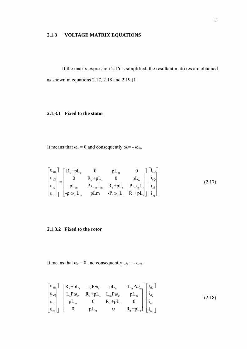
2.1.3 VOLTAGE MATRIX EQUATIONS
If the matrix expression 2.16 is simplified, the resultant matrixes are obtained
as shown in equations 2.17, 2.18 and 2.19.[1]
2.1.3.1 Fixed to the stator.
It means that ωs = 0 and consequently ωr= - ωm.
sD sDs s m
sQ sQs s m
m m m r r m rrd rd
m m m r r rrq rq
u iR +pL 0 pL 0u i0 R +pL 0 pL
=pL P.ω L R +pL P.ω Lu i
-p.ω L pLm -P.ω L R +pLu i
⎡ ⎤ ⎡⎡ ⎤⎢ ⎥ ⎢⎢ ⎥⎢ ⎥ ⎢⎢⎢ ⎥ ⎢⎢⎢ ⎥ ⎢⎢ ⎥
⎢ ⎥⎢ ⎥ ⎢⎣ ⎦⎣ ⎦ ⎣
.
⎤⎥⎥⎥⎥⎥⎥⎥⎦
.
⎤⎥⎥⎥⎥⎥⎥⎥⎦
(2.17)
2.1.3.2 Fixed to the rotor
It means that ωr = 0 and consequently ωs = - ωm.
sD sDs s s m m m m
sQ sQs m s s m m m
m r rrd rd
m r rrq rq
u iR +pL -L P pL -L Pu iL P R +pL L P pL
=pL 0 R +pL 0u i
0 pL 0 R +pLu i
ω ωω ω
⎡ ⎤ ⎡⎡ ⎤⎢ ⎥ ⎢⎢ ⎥⎢ ⎥ ⎢⎢⎢ ⎥ ⎢⎢⎢ ⎥ ⎢⎢ ⎥
⎢ ⎥⎢ ⎥ ⎢⎣ ⎦⎣ ⎦ ⎣
(2.18)
16
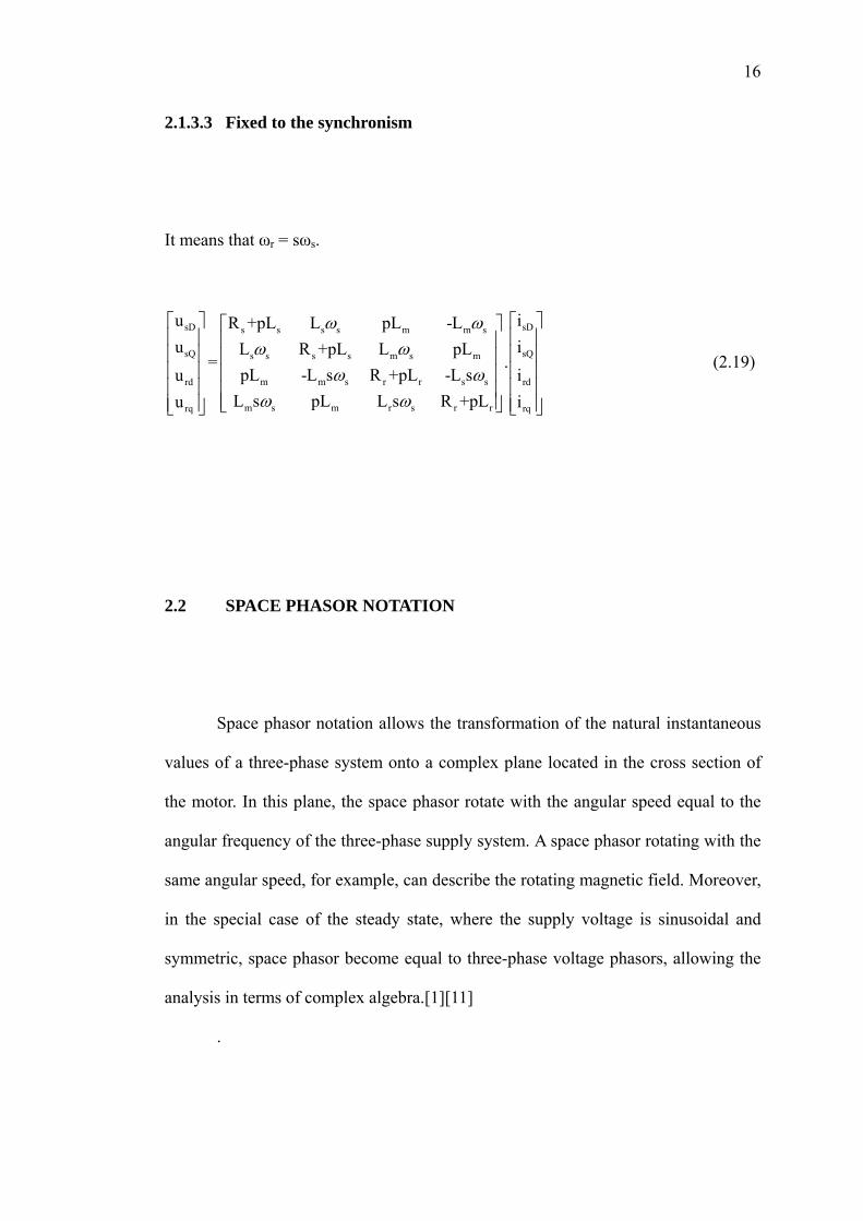
2.1.3.3 Fixed to the synchronism
It means that ωr = sωs.
sD sDs s s s m m s
sQ sQs s s s m s m
m m s r r s srd rd
m s m r s r rrq rq
u iR +pL L pL -Lu iL R +pL L pL
=pL -L s R +pL -L su i
L s pL L s R +pLu i
ω ωω ω
ω ωω ω
⎡ ⎤ ⎡⎡ ⎤⎢ ⎥ ⎢⎢ ⎥⎢ ⎥ ⎢⎢⎢ ⎥ ⎢⎢⎢ ⎥ ⎢⎢ ⎥
⎢ ⎥⎢ ⎥ ⎢⎣ ⎦⎣ ⎦ ⎣
.
⎤⎥⎥⎥⎥⎥⎥⎥⎦
(2.19)
2.2 SPACE PHASOR NOTATION
Space phasor notation allows the transformation of the natural instantaneous
values of a three-phase system onto a complex plane located in the cross section of
the motor. In this plane, the space phasor rotate with the angular speed equal to the
angular frequency of the three-phase supply system. A space phasor rotating with the
same angular speed, for example, can describe the rotating magnetic field. Moreover,
in the special case of the steady state, where the supply voltage is sinusoidal and
symmetric, space phasor become equal to three-phase voltage phasors, allowing the
analysis in terms of complex algebra.[1][11]
.
17
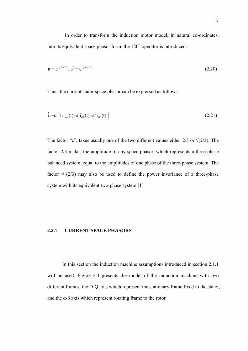
In order to transform the induction motor model, in natural co-ordinates,
into its equivalent space phasor form, the 120° operator is introduced:
j 2π / 3 2 j 4π / 3a = e , a = e (2.20)
Thus, the current stator space phasor can be expressed as follows:
2s sA sB sCi =c. 1.i (t)+a.i (t)+a i (t)⎡⎣ ⎤⎦ (2.21)
The factor “c”, takes usually one of the two different values either 2/3 or √(2/3). The
factor 2/3 makes the amplitude of any space phasor, which represents a three phase
balanced system, equal to the amplitudes of one phase of the three-phase system. The
factor √ (2/3) may also be used to define the power invariance of a three-phase
system with its equivalent two-phase system.[1]
2.2.1 CURRENT SPACE PHASORS
In this section the induction machine assumptions introduced in section 2.1.1
will be used. Figure 2.4 presents the model of the induction machine with two
different frames, the D-Q axis which represent the stationary frame fixed to the stator,
and the α-β axis which represent rotating frame to the rotor.
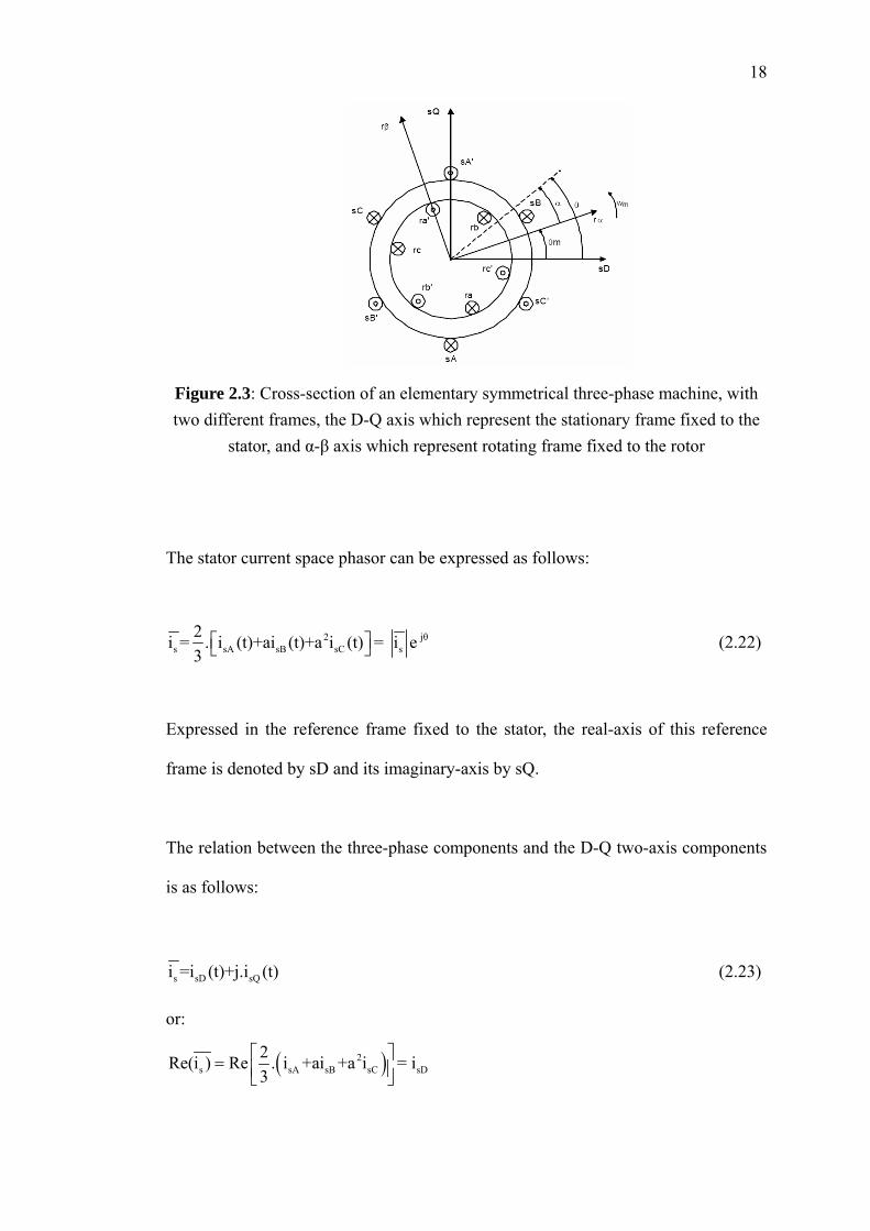
18
Figure 2.3: Cross-section of an elementary symmetrical three-phase machine, with two different frames, the D-Q axis which represent the stationary frame fixed to the
stator, and α-β axis which represent rotating frame fixed to the rotor
The stator current space phasor can be expressed as follows:
2 θs sA sB sC s
2i = . i (t)+ai (t)+a i (t) = i e3⎡⎣
j⎤⎦ (2.22)
Expressed in the reference frame fixed to the stator, the real-axis of this reference
frame is denoted by sD and its imaginary-axis by sQ.
The relation between the three-phase components and the D-Q two-axis components
is as follows:
s sD sQi =i (t)+j.i (t) (2.23)
or:
( )2s sA sB sC
2Re(i ) Re . i +ai +a i = i3⎡ ⎤= ⎢ ⎥⎣ ⎦
sD
19
( )2s sA sB sC
2Im(i ) Im . i +ai +a i = i3⎡= ⎢⎣ ⎦
sQ⎤⎥ (2.24)
The relationship between the space phasor current and the real stator phase current
can be expressed as follows:
2s sA sB sC
2R e(i ) Re . i +ai +a i = i3⎡ ⎤⎡ ⎤= ⎣ ⎦⎢ ⎥⎣ ⎦
sA
2 2s sA sB sC
2Re( i ) Re . i +i + i = i3
a a a⎡ ⎡ ⎤= ⎣ ⎦⎢⎣ ⎦sB
⎤⎥ (2.25)
2s sA sB sC
2Re( .i ) Re . i + i +i = i3
a a a⎡ ⎤⎡ ⎤= ⎣ ⎦⎢ ⎥⎣ ⎦sC
In a similar way, the space phasor of the rotor current can be written as follows:
2r ra rb rc r
2i = . i (t) + ai (t) + a i (t) = i e 3
jα⎡⎣ ⎤⎦ (2.26)
Expressed in the reference frame fixed to the rotor, the real –axis of this reference
frame is denoted by rα and its imaginary-axis by rβ.
The space phasor of the rotor current expressed in the stationary reference frame
fixed to the stator can be expressed as follows:
m j ( α + θ ) jθr r ri' = i e = i e (2.27)
The relation between the current rotor space phasor and the α-β two-axis is as
follows:
20
r rα rβi = i (t) + j.i (t) (2.28)
or:
( )2r ra rb rc
2Re(i ) Re . i +ai +a i = i3 rα⎡ ⎤= ⎢ ⎥⎣ ⎦
( )2r ra rb rc
2Im(i ) Im . i +ai +a i = i3 rβ⎡= ⎢⎣ ⎦
⎤⎥ (2.29)
The relationship between the space phasor current and the real stator currents can be
expressed as follows:
2r ra rb rc
2Re(i ) Re . i +ai +a i =i3 rα⎡ ⎤⎡ ⎤= ⎣ ⎦⎢ ⎥⎣ ⎦
2 2r ra rb rc
2Re( i ) Re . i +i + i =i3
a a a⎡ ⎤⎡ ⎤= ⎣ ⎦⎢ ⎥⎣ ⎦rb
2r ra rb rc
2Re( i ) Re . i + i +i =i3
a a a⎡ ⎡= ⎣⎢⎣ ⎦rc
⎤⎤⎦⎥ (2.30)
The magnetizing current space-phasor expressed in the stationary reference frame
fixed to the stator can be obtained as follows:
si i i'rem
se
NN
⎛= + ⎜⎝ ⎠ r
⎞⎟ (2.31)
21
2.2.2 FLUX LINKAGE SPACE PHASOR
In this section the flux linkage will be formulated in the stator phasor notation
according to the different reference frames.
2.2.2.1 Stator flux-linkage space phasor in the stationary reference frame fixed
to the stator.
Similar to the definitions of the stator current and the rotor current space phasors, it
is possible to define a space phasor for the flux linkage as follows:
( 2s sA sB s
2ψ = ψ +aψ +a ψ3
)C (2.32)
If the flux linkage equations 2.7, 2.8, 2.9 are substituted in equation 2.32, the space
phasor for the stator flux linkage can be expressed as follows:
( ) ( ) ( )( )( )( )
2 2 2
2
2
2
cos cos( 4 / 3) cos( 2 / 3)23 cos cos( 2 / 3) cos( 4 / 3)
cos cos( 2 / 3) cos( 4 / 3)
sA s s s sB s s s sC s s s
ra sr m sr m sr ms
rb sr m sr m sr m
rc sr m sr m sr m
i L aM a M i aL M a M i a L M aM
i M aM a M
i aM M a M
i a M aM M
θ θ π θ π
θ θ π θ π
θ θ π θ π
⎡ + + + + + + + + +⎢⎢+ + + + + +⎢Ψ = ⎢+ + + + + +⎢
+ + + + +⎣
⎤⎥⎥⎥⎥⎥
⎢ ⎥⎢ ⎥⎦
(2.33)
Developing the previous expression 2.33, it is obtained the following expression:
22
( ) ( ) ( )( )( )( )
2 2 2 2
2
2
2 2
.
cos cos( 4 / 3) cos( 2 / 3)23 . cos cos( 2 / 3) cos( 4 / 3)
. cos cos( 2 / 3) cos( 4 / 3)
sA s s s sB s s s sC s s s
ra sr m sr m sr m
s
rb sr m sr m sr m
rc sr m sr m sr m
i L aM a M a i L aM a M a i L a M aM
i M aM a M
a i M a M aM
a i M a M aM
θ θ π θ π
θ θ π θ π
θ θ π θ π
⎡ + + + + + + + +
+ + + + +Ψ =
+ + + + +
+ + + + +
⎤⎢ ⎥⎢ ⎥⎢ ⎥⎢ ⎥⎢ ⎥⎢ ⎥⎢ ⎥⎣ ⎦
(2.34)
And finally, expression 2.34 can be expressed as follows:
( ) ( )2 2s s s s s sr m sr m sr mΨ = L +aM +a M i + M cosθ +aM cos(θ +4π/3)+a M cos(θ +2π/3) ir
( ) ( ) ( )mjθs s s m sr r s s s sr r s s s sr = L -M i +1.5cosθ M i = L -M i +1.5e M i = L -M i +1.5M i 'r
s s m r = L i +L i ' (2.35)
where Ls is the total three-phase stator inductance and the Lm is the so-called
three-phase magnetizing inductance. Finally, the space phasor of the flux linkage in
the stator depends on two components, being the stator currents and the rotor
currents.
Once more, the flux linkage magnitude can be expressed in two-axis as follows:
s sD sψ = ψ + j.ψ Q
.i
(2.36)
Where its direct component is equal to:
sD s sD m rdψ = L .i + L (2.37)
And its quadrature component is expressed as:
23
sQ s sQ m rqψ = L .i + L .i (2.38)
The relationship between the components ird and irα and irq and irβ may be introduced
as follows:
m j θr rd rq ri' = i + j.i = i . e (2.39)
The compactness of the notation in the space phasor nomenclature compared to the
two-axis notation in 1.1 is noticeable.
2.2.2.2 Rotor flux-linkage space phasor in the rotating reference frame fixed to
the rotor.
The rotor flux linkage space phasor, fixed to the rotor natural frame ca be defined as
follows:
( 2s ra rb
2ψ = ψ +aψ +a ψ3
)rc (2.40)
If the flux linkage equations 2.10, 2.11, 2.12 are substituted in equation 2.40, the
space phasor for the rotor flux linkage can be expressed as follows:
( ) ( ) ( )( )( )( )
2 2 2ra r r r rb r r r rc r r r
2sA sr m sr m sr m
r2
sB sr m sr m sr m
2sC sr m sr m sr m
i L +aM +a M +i aL +M +a M +i a L +M +aM +
+i M cosθ +aM cos(θ +4π/3)+a M cos(θ +2π/3) +2Ψ =3 +i aM cosθ +M cos(θ +4π/3)+a M cos(θ +2π/3) +
+i a M cosθ +aM cos(θ +4π/3)+M cos(θ +2π/3)
⎡⎢⎢⎢⎢⎢
⎣
⎤⎥⎥⎥⎥⎥
⎢ ⎥⎢ ⎥⎦
(2.41)
24
By re-arranging the previous expression 2.41, it can be expressed as:
( ) ( ) ( )( )( )( )
2 2 2 2ra r r r rb r r r rc r r r
2sa sr m sr m sr m
s 2sb sr m sr m sr m
2 2sc sr m sr m sr m
i L +aM +a M +a.i L +aM +a M +a i L +a M +aM
+i M cosθ +aM cos(θ +4π/3)+a M cos(θ +2π/3)2Ψ =3 +a.i M cosθ +a M cos(θ +4π/3)+aM cos(θ +2π/3)
+a .i M cosθ +a M cos(θ +4π/3)+aM cos(θ +2π/3)
⎡ ⎤⎢ ⎥⎢ ⎥⎢ ⎥⎢ ⎥⎢ ⎥⎢ ⎥⎢ ⎥⎣ ⎦
(2.42)
And finally:
( ) ( )2 2r r r r r sr m sr m sr mΨ = L +aM +a M i + M cosθ +aM cos(θ +2π/3)+a M cos(θ +4π/3) is
( ) ( ) ( )m-jθr r r m sr s r r r sr s r r r sr= L -M i +1.5cos(-θ )M i = L -M i +1.5e M i = L -M i +1.5M i 's
r r m s= L i +L i ' (2.43)
where si is the stator current space phasor expressed in the frame fixed to the rotor.
Again, the flux linkage magnitude can be expressed in the two-axis form as
follows:
r rα rβψ = ψ + j.ψ (2.44)
Where its direct component is equal to:
rα r rα m sαψ = L .i + L .i (2.45)
And its quadrature component is expressed as:
rβ r rβ m sβψ = L .i + L .i (2.46)
25
2.2.2.3 Rotor flux-linkage space phasor in the stationary reference frame fixed
to the stator.
The rotor flux linkage can also be expressed in the stationary reference frame using
the previously introduced transformation , and can be written as: j. θ me
( )mjθ j ( α + θ )r rd rq r rα rβψ' = ψ + j.ψ = ψ .e = ψ + j.ψ e m (2.47)
The space phasor of the rotor flux linkage can be expressed according to the fixed
co-ordinates as follows:
mj θr r r m s r r mψ' = L .i' + L .i 'e = L .i + L .is (2.48)
The relationship between the stator current referred to the stationary frame fixed to
the stator and the rotational frame fixed to the rotor is as follows:
m
m
j θs s
-jθs s
i = i '.e
i .e = i ' (2.49)
where
s sD s
s sα sβ
i = i + j.i
i' = i + j.iQ (2.50)
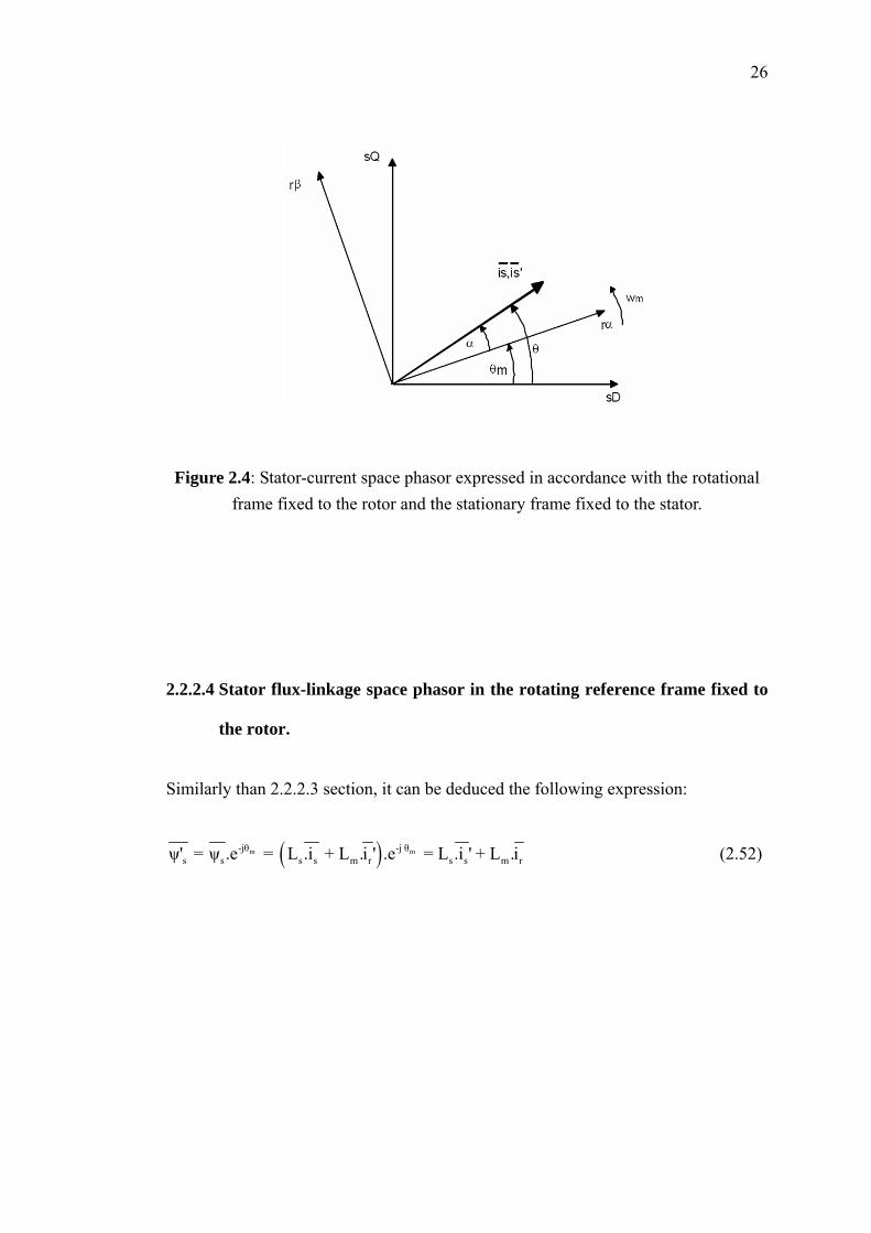
From figure 2.5, the following equivalencies can be deduced:
m m
jθs s
j ( θ - θ ) - θjαs s s s
i = i .e
i ' = i ' .e = i ' .e = i .e j (2.51)
26
Figure 2.4: Stator-current space phasor expressed in accordance with the rotational frame fixed to the rotor and the stationary frame fixed to the stator.
2.2.2.4 Stator flux-linkage space phasor in the rotating reference frame fixed to
the rotor.
Similarly than 2.2.2.3 section, it can be deduced the following expression:
( )m m-jθ -j θs s s s m r s s m rψ' = ψ .e = L .i + L .i ' .e = L .i ' + L .i (2.52)
27
2.2.3 THE SPACE PHASORS OF STATOR AND ROTOR VOLTAGES
The space phasors for the stator and the rotor voltages can be defined in a similar way
like the one used for other magnitudes.
( )
( )
2s sA sB sC sD sQ sA sB sC sB
2r ra rb rc rα rβ ra rb rc rb rc
2 2 1 1u = . u (t) + ai (t) + a i (t) = u + j.u = u - u - u + j u -u3 3 2 2 32 2 1 1u = . u (t) + a.i (t) + a i (t) = u + j.u = . u - u - u + j. . u -u3 3 2 2 3
⎛ ⎞⎡ ⎤ ⎜ ⎟⎣ ⎦ ⎝ ⎠⎛ ⎞⎡ ⎤ ⎜ ⎟⎣ ⎦ ⎝ ⎠
sC1
1
(2.53)
where the stator voltage space phasor is referred to the stationary reference frame and
the rotor voltage space phasor is referred to the rotating frame fixed to the rotor.[1]
Provided the zeros component is zero, it can also be said that:
( )( )( )
sA s
2sB s
sC s
u =Re u
u =Re a u
u =Re au
(2.54)
Equivalent expressions can also be obtained for the rotor.
28
2.2.4 SPACE-PHASOR FORM OF THE MOTOR EQUATIONS
The space phasor forms of the voltage equations of the three-phase and
quadrature -phase smooth air-gap machines will be presented. The equations will be
expressed in a general rotating reference frame, which rotates at a general speed,
and then to the references frames fixed to the stator, rotor, and synchronous speed.
gω
2.2.4.1 Space phasor voltage equation in the general reference frame
If the voltage in the figure 2.6 is the stator current, then its formulation in the space
phasor form is as follows [11]:
g- j θsg s sxi = i .e = i + j sy.i (2.55)
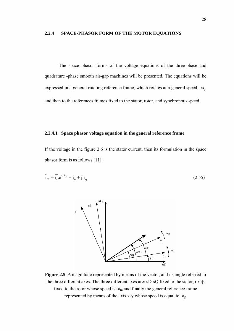
Figure 2.5: A magnitude represented by means of the vector, and its angle referred to the three different axes. The three different axes are: sD-sQ fixed to the stator, rα-rβ
fixed to the rotor whose speed is ωm and finally the general reference frame represented by means of the axis x-y whose speed is equal to ωg.
29
In a similar way and for other magnitudes, it can be written the following equations:
g
g
- j θsg s sx sy
- j θsx sysg s
u = u .e = u + j.u
ψ = ψ .e = ψ + j.ψ (2.56)
where the magnitudes are the voltage space phasor and the stator flux linkage
respectively.
However, if the magnitude in the figure 2.6 is for instance the rotor current, its space
phasor notation will be:
g m-j.(θ -θ )rg r rxi = i e = i + ryj.i (2.57)
and for other magnitudes:
g m
g m
- j (θ -θ )rg r rx ry
- j (θ -θ )rx ryrg r
u = u .e = u + j.u
ψ = ψ .e = ψ + j.ψ (2.58)
Manipulating the previous equations yields the following stator and rotor space
phasor voltage equations in the general reference frame.
( )
( )
g
g g g g
g m
g m g m
g m g m g m
jθsgj θ jθ jθ jθsg
sg s sg s sg g sg
j.(θ -θ )rj (θ -θ ) j.(θ -θ )
rg r rg
j(θ -θ ) j ( θ -θ ) j(θ -θ )rgr rg g m rg
d ψ e dψu .e = R .i e + = R .i e + + j.e ω ψ
dt dtd ψ e
u .e = R .i .e +dt
dψ = R .i .e + e + j.e (ω -P.ω ).ψ
dt
(2.59)
30
Simplifying equation 2.59, it will result as equation 2.60.
sgsgsg s g sg
rgrgrg r g
dψu = R .i + + j.ω .ψ
dtdψ
u = R .i + + j.(ω -P.ω ).ψdt m rg
(2.60)
Where, the flux linkage space phasors are:
sg rgs msg
rg sgr mrg
ψ = L .i + L .i
ψ = L .i + L .i (2.61)
Using the two-axis notation and the matrix form, the voltage equations can be
represented by:
sx sxs s s g m m g
sy sys g s s m g m
m m m g r r r g mrx rx
m g m m r g m r rry ry
u iR +pL -L ω pL -L ωu iL ω R +pL L ω pL
= .pL L (P.ω -ω ) R +pL L (-ω +P.ω )u i
L (ω -P.ω ) pL L (w -P.w ) R +pLu i
⎡ ⎤ ⎡ ⎤⎡ ⎤⎢ ⎥ ⎢ ⎥⎢ ⎥⎢ ⎥ ⎢ ⎥⎢ ⎥⎢ ⎥ ⎢ ⎥⎢ ⎥⎢ ⎥ ⎢ ⎥⎢ ⎥
⎢ ⎥⎢ ⎥ ⎢ ⎥⎣ ⎦⎣ ⎦ ⎣ ⎦
(2.62)
2.2.4.2 Space-phasor voltage equations in the stationary reference frame fixed
to the stator
If ω g=0, equation 2.18 can be expressed as equation 2.67.
31
sD sDs s m
sQ sQs s m
m m m r r m rrd rd
m m m m r r rrq rq
u iR +pL 0 pL 0u i0 R +pL 0 pL
=pL P.ω L R +pL P.ω Lu i
-p.ω L pL -P.ω L R +pLu i
⎡ ⎤ ⎡⎡ ⎤⎢ ⎥ ⎢⎢ ⎥⎢ ⎥ ⎢⎢⎢ ⎥ ⎢⎢⎢ ⎥ ⎢⎢ ⎥
⎢ ⎥⎢ ⎥ ⎢⎣ ⎦⎣ ⎦ ⎣
.
⎤⎥⎥⎥⎥⎥⎥⎥⎦
(2.63)
The stator voltage space phasor can be expressed as follows:
ss s s
dψu = R .i + dt
(2.64)
The rotor voltage space phasor can be expressed as follows:
( )m
m
-jθr-jθ- j θm
r r r
rr r r m r
d ψ' eu' .e = R .i' e +
dtdψ'u' = R .i ' + + j.P.ω ψ'dt
(2.65)
And the flux linkage space phasor can be expressed as follows:
ss ms
r sr mr
ψ = L .i + L .i'
ψ' = L .i' + L .ir
m
(2.66)
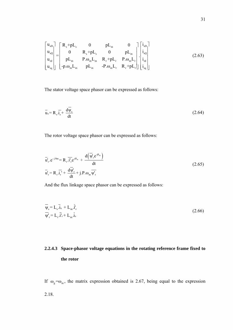
2.2.4.3 Space-phasor voltage equations in the rotating reference frame fixed to
the rotor
If , the matrix expression obtained is 2.67, being equal to the expression
2.18.
gω =ω
32
sD sDs s s m m m m
sQ sQs m s s m m m
m r rrd rd
m r rrq rq
u iR +pL -L Pω pL -L Pωu iL Pω R +pL L Pω pL
=pL 0 R +pL 0u i
0 pL 0 R +pLu i
⎡ ⎤ ⎡⎡ ⎤⎢ ⎥ ⎢⎢ ⎥⎢ ⎥ ⎢⎢⎢ ⎥ ⎢⎢⎢ ⎥ ⎢⎢ ⎥
⎢ ⎥⎢ ⎥ ⎢⎣ ⎦⎣ ⎦ ⎣
.
⎤⎥⎥⎥⎥⎥⎥⎥⎦
(2.67)
The stator voltage space phasor can be expressed as follows:
ss s s m
dψ'u' = R .i' + + j.P.ω ψ'dt s (2.68)
The rotor voltage space phasor can be expressed as follows:
rr rr
dψu = R .i + dt
(2.69)
And the flux linkage space phasor can be expressed as follows:
rs s s m
rr mr
ψ' = L .i' + L .i
ψ = L .i + L .i's
s
(2.70)
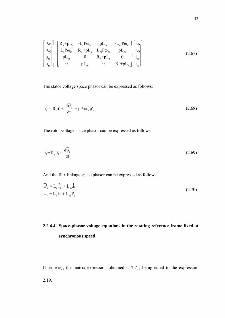
2.2.4.4 Space-phasor voltage equations in the rotating reference frame fixed at
synchronous speed
If , the matrix expression obtained is 2.71, being equal to the expression
2.19.
gω ω=

33
sD sDs s s s m m s
sQ sQs s s s m s m
m m s r r s srd rd
m s m r s r rrq rq
u iR +pL L ω pL -L ωu iL ω R +pL L ω pL
=pL -L sω R +pL -L sωu i
L sω pL L sω R +pLu i
⎡ ⎤ ⎡⎡ ⎤⎢ ⎥ ⎢⎢ ⎥⎢ ⎥ ⎢⎢⎢ ⎥ ⎢⎢⎢ ⎥ ⎢⎢ ⎥
⎢ ⎥⎢ ⎥ ⎢⎣ ⎦⎣ ⎦ ⎣
.
⎤⎥⎥⎥⎥⎥⎥⎥⎦
(2.71)
The stator voltage space phasor can be expressed as follows:
sgsgsg s sg
dψu = R .i + + j.ω ψ
dt s (2.72)
The rotor voltage space phasor can be written as follows:
rgrgrg r s rg
dψu = R .i + + j.(ω -P.ω ).ψ
dt m (2.73)
And the flux linkage space phasor can be expressed as follows:
sg rgs msg
rg sgr mrg
ψ = L .i + L .i
ψ = L .i + L .i (2.74)
34
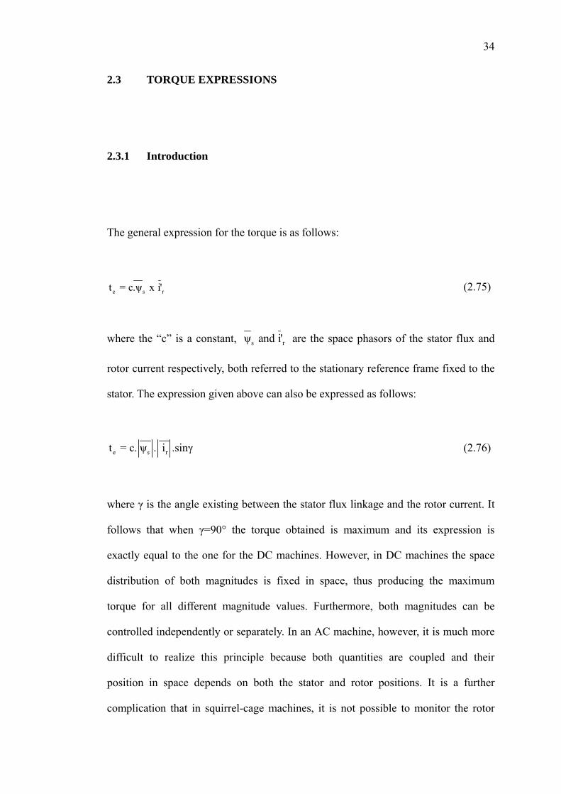
2.3 TORQUE EXPRESSIONS
2.3.1 Introduction
The general expression for the torque is as follows:
e st = c.ψ x i'r (2.75)
where the “c” is a constant, rsψ and i' are the space phasors of the stator flux and
rotor current respectively, both referred to the stationary reference frame fixed to the
stator. The expression given above can also be expressed as follows:
e s rt = c. ψ . i .sinγ (2.76)
where γ is the angle existing between the stator flux linkage and the rotor current. It
follows that when γ=90° the torque obtained is maximum and its expression is
exactly equal to the one for the DC machines. However, in DC machines the space
distribution of both magnitudes is fixed in space, thus producing the maximum
torque for all different magnitude values. Furthermore, both magnitudes can be
controlled independently or separately. In an AC machine, however, it is much more
difficult to realize this principle because both quantities are coupled and their
position in space depends on both the stator and rotor positions. It is a further
complication that in squirrel-cage machines, it is not possible to monitor the rotor
35
current, unless the motor is specially prepared for this purpose in a special laboratory.
It is impossible to find them in a real application. The search for a simple control
scheme similar to the one for DC machines has led to the development of the
so-called vector-control schemes, where the point of obtaining two different currents,
one for controlling the flux and the other one for the rotor current is achieved.
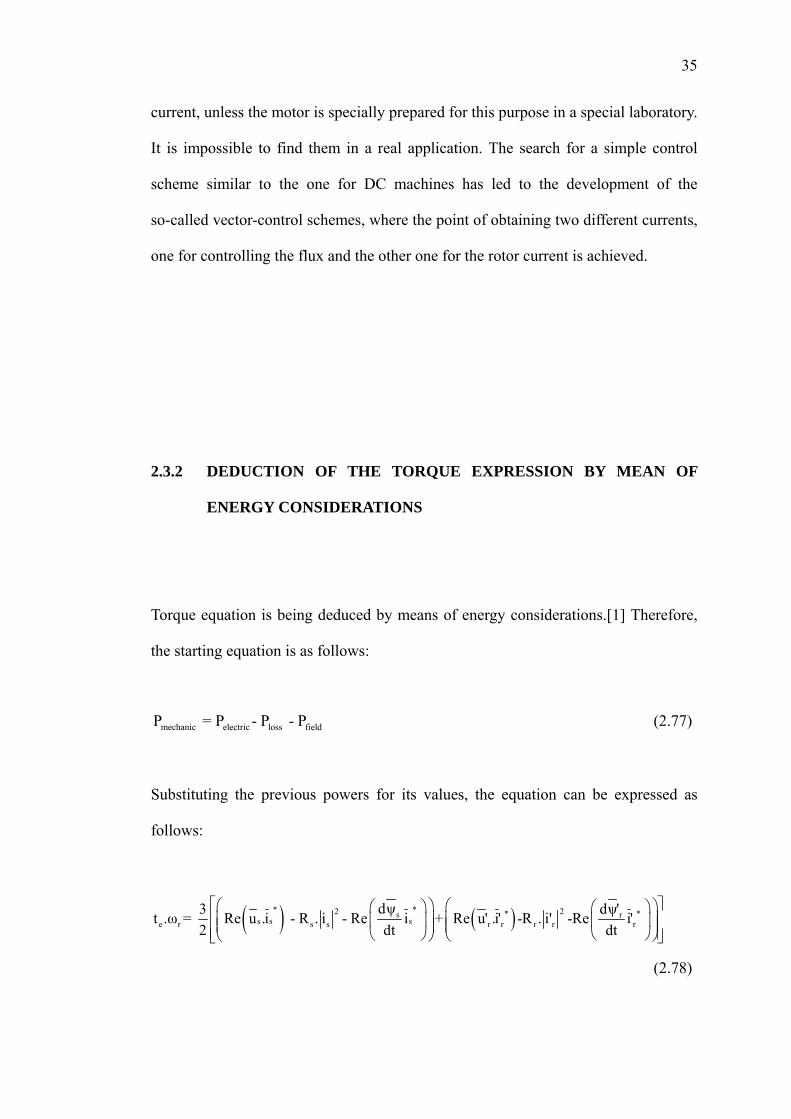
2.3.2 DEDUCTION OF THE TORQUE EXPRESSION BY MEAN OF
ENERGY CONSIDERATIONS
Torque equation is being deduced by means of energy considerations.[1] Therefore,
the starting equation is as follows:
mechanic electric loss fieldP = P - P - P (2.77)
Substituting the previous powers for its values, the equation can be expressed as
follows:
( ) ( )* *2 2* *s rs sse r s s r r r r r
dψ dψ'3t .ω = Re u .i - R . i - Re i + Re u' .i' -R . i' -Re i'2 dt
⎡ ⎤⎛ ⎞ ⎛ ⎞⎛ ⎞ ⎛ ⎞⎢ ⎥⎜ ⎟ ⎜ ⎟⎜ ⎟ ⎜ ⎟⎜ ⎟⎜ ⎟⎢ ⎥⎝ ⎠⎝ ⎠ ⎝ ⎠⎝ ⎠⎣ ⎦dt
(2.78)
36
Since in the stationary reference frame, the stator voltage space phasor us can only
balanced by the stator ohmic drop, plus the rate of change of the stator flux linkage,
previous expression can be expressed as follows:
( ) ( )* *e r r r r r r r r r r
3 3 3t .ω = .Re - j.ω ψ' i' = - ω .Re j ψ' i' = - ω .ψ' x i'2 2 2
(2.79)
Expressing the equation in a general way for any number of pair of poles given:
e r3t = - .P.ψ' x i'2 r (2.80)
If equation 2.66 and 2.35 are substituted in equation 2.80, it is obtained the following
expression for the torque:
se s3t = .P.ψ x i2
(2.81)
If the product is developed, expression 2.81 is as follows:
e sD sQ sQ3t = P(ψ .i -ψ .i )2 sD (2.82)
Finally, different expressions for the torque can be obtained as follows:
s s re r r m r m r m s
m m mse m r s r rs s2
s s s r
3 3 3t = - P(L i' +L i ) x i' = - PL i x i' = - PL i' x i2 2 2
L 3L L3 3t = - P (L i' +L i ) x i' = - P ψ x i' = - P ψ x ψ'2 L 2L 2 L L - L r
m
(2.83)
37
CHAPTER 3
DIRECT TORQUE CONTROL: PRINCIPLES AND
GENERALITIES
3.1 INDUCTION MOTOR CONTROLLERS
3.1.1 Voltage /Frequency
There are too many different ways to drive an induction motor. The main
differences between them are the motor’s performance and the viability and cost in
its real implementation. Despite the fact that –‘Voltage /Frequency’ (V/Hz) is the
simplest controller, it is the most widespread, being in the majority of the industrial
38
applications. It is known as a scalar control and acts imposing a constant relation
between voltage and frequency.
The structure is very simple and it is normally used without speed feedback.
However, this controller does not achieve a good accuracy in both speed and torque
response mainly due to the fact that the stator flux and the torque are not directly
controlled. Even though, as long as the parameters are identified, the accuracy in the
speed can be 2% (except in a very low speed) and dynamic response can be
approximately around 50ms.[3][4][33]
3.1.2 Vector controls.
According to these types of controllers, there are control loops for
controlling both the torque and the flux.[5] The most widespread controllers are the
ones that use vector transform such as either Park or Ku. Its accuracy can reach
values such as 0.5% regarding the speed and 2% regarding the torque, even in stand
still. The main disadvantages are the huge computational capability required and the
compulsory good identification of motor parameters.[6][33]
39
3.1.3 Field Acceleration method.
The equation used in this method can be simplified avoiding the vector
transformation. It is achieved some computational reduction, overcoming the main
problem in the vector controllers and then becoming an important alternative for the
vector controllers.[10][6][8]
3.1.4 Direct Torque Control.
In direct torque control (DTC), it is possible to control directly the stator flux
and the torque by selecting the appropriate inverter switching state [12][11].
Its main features are as follows:
Direct torque control and direct stator flux control.
Indirect control of stator currents and voltages.
Approximately sinusoidal stator fluxes and stator currents
High dynamic performance even at locked rotor.
This method presents the following advantages:
Absences of co-ordinates transform.
Absences of mechanical transducers.
40
Current regulators, PWM pulse generation, PI control of flux and torque and
co-ordinate transformation are not required.
Very simple control scheme and low computation time.
Reduced parameters sensitivity.
Very good dynamic properties.
Although, some disadvantages are present:
High torque ripples and current distortions
Low switching frequency of transistors with relation to computation time
Constant error between reference and real torque
3.2 PRINCIPLES OF DIRECT TORQUE CONTROL
3.2.1 Introduction
As it has been introduced in expression 1.81, the electromagnetic torque in
the three-phase induction machines can be expressed as follows [11][13]:
41
e s3t = PΨ x i2
uur urs (3.1)
where is the stator flux, sΨuur
sir
is the stator current(both fixed to the stationary
reference frame fixed to the stator) and P the number of pair of poles. The previous
equation can be modified and expressed as follows:
s s3 P . .sin(α - ρ )2e s st i= Ψ
uuur ur (3.2)
where is the stator flux angle and α is the stator current one, both referred to the
horizontal axis of the stationary frame fixed to the stator. If the stator flux modulus is
kept constant and the angle sρ is changed quick then the electromagnetic torque is
directly controlled.
sρ s
ly,
The same conclusion can be made by using another expression for the
electromagnetic torque. From equation 1.83, next equation can be written as:
'ms r2
s r m
L3 P x .sin(ρ - ρ )2 L L Le r st = Ψ Ψ
−
uuur uuur (3.3)
The fact that the rotor flux can be assumed constant is true as long as the
response time of the control is much faster than the rotor time constant. As long as
the stator flux modulus is kept constant, then the electromagnetic torque can be
rapidly changed and controlled by means of changing the angle .[7][14] s r(ρ - ρ )
42
3.2.2 DTC Controller
The way to impose the require stator flux is by means of choosing the most
suitable Voltage Source Inverter state. If the ohmic drops are neglected for simplicity,
then the stator voltage impresses directly the stator flux in accordance with the
following equation:
ss
d udtΨ
=uuur
(3.4)
or
s su t∆Ψ = ∆uuur
(3.5)
Decoupled control of the stator flux modulus and the torque is achieved by
acting on the radial and tangential components respectively of the stator flux-linkage
space vector in its locus. These two components are directly proportional (Rs =0) to
the components of the same voltage space vector in the same directions. Figure 3.1
shows the possible dynamics locus of the stator flux, and its different variation
depending on the VSI states chosen. The possible global locus is divided into six
different sectors signaled by the discontinuous line.
43
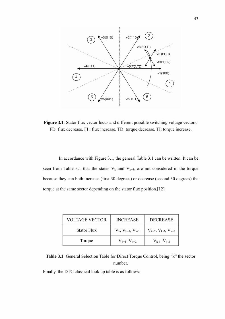
Figure 3.1: Stator flux vector locus and different possible switching voltage vectors. FD: flux decrease. FI : flux increase. TD: torque decrease. TI: torque increase.
In accordance with Figure 3.1, the general Table 3.1 can be written. It can be
seen from Table 3.1 that the states Vk and Vk+3, are not considered in the torque
because they can both increase (first 30 degrees) or decrease (second 30 degrees) the
torque at the same sector depending on the stator flux position.[12]
VOLTAGE VECTOR INCREASE DECREASE
Stator Flux Vk, Vk+1, Vk-1 Vk+2, Vk-2, Vk+3
Torque Vk+1, Vk+2 Vk-1, Vk-2
Table 3.1: General Selection Table for Direct Torque Control, being “k” the sector
number.
Finally, the DTC classical look up table is as follows:

44
Φ τ S1 S2 S3 S4 S5 S6
TI V V V V V V
T= V2 V3 V4 V5 V6 V1
FI
TD V0 V7 V0 V7 V0 V7
TI V3 V4 V5 V6 V1 V2
T= V7 V0 V7 V0 V7 V0
FD
TD V5 V6 V1 V2 V3 V4
Table 3.2: Look up table for Direct Torque Control. FD/FI: flux decrease/increase. TD/=/: torque decrease/equal/increase. Sx: stator flux sector.Φ : stator flux modulus
error after the hysteresis block.τ : torque error after the hysteresis block.
The sectors of the stator flux space vector are denoted from S1 to S6. Stator
flux modulus error after the hysteresis block (Φ ) can take just two values. Torque
error after the hysteresis block (τ ) can take three different values. The zero voltage
vectors V0 and V7 are selected when the torque error is within the given hysteresis
limits, and must remain unchanged.
45
3.2.3 DTC Schematic.
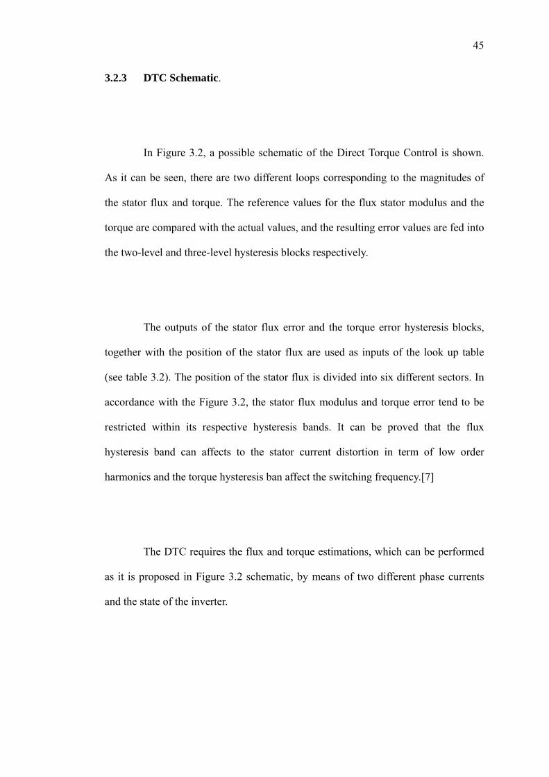
In Figure 3.2, a possible schematic of the Direct Torque Control is shown.
As it can be seen, there are two different loops corresponding to the magnitudes of
the stator flux and torque. The reference values for the flux stator modulus and the
torque are compared with the actual values, and the resulting error values are fed into
the two-level and three-level hysteresis blocks respectively.
The outputs of the stator flux error and the torque error hysteresis blocks,
together with the position of the stator flux are used as inputs of the look up table
(see table 3.2). The position of the stator flux is divided into six different sectors. In
accordance with the Figure 3.2, the stator flux modulus and torque error tend to be
restricted within its respective hysteresis bands. It can be proved that the flux
hysteresis band can affects to the stator current distortion in term of low order
harmonics and the torque hysteresis ban affect the switching frequency.[7]
The DTC requires the flux and torque estimations, which can be performed
as it is proposed in Figure 3.2 schematic, by means of two different phase currents
and the state of the inverter.
46
Figure 3.2: Direct Torque Control Schematic.
However, flux and torque estimations can be performed using other
magnitudes such as two stator currents and the mechanical speed, or two stator
currents again and the shaft position.[14][12]
3.2.3.1 Stator flux and torque estimator using , isA and isB magnitudes. mω
This estimator does not require co-ordinate transform. It is used the motor
model fixed to the stationary reference frame fixed to the stator. Firstly, all
three-phase currents must be converted into its D and Q components. By means of
the Park transformation defined in equation 1.14, it can be assumed:
sD sAi c.1.5.i=
47
sQ sB sAi c. 3/2.(2.i i= )+ (3.6)
If rotor current is extracted from equation 2.65 and substituted into equation 2.66, it
can be said:
r r mr
r r
L L Pω' .(1+p. )=L iR R
jΨ − m s (3.7)
And if the expression 3.7 is arranged:
sr r r m r r r' .(R +p.L )=L R .i +j. ' .L .P.ωΨ Ψ m (3.8)
Expanding the previous equation into its D and Q components, it obtained:
sDrD r r m r rQ r m' .(R +p.L )=L R .i +j. ' .L .P.ωΨ Ψ (3.9)
sQrQ r r m r rD r m' .(R +p.L )=L R .i +j. ' .L .P.ωΨ Ψ (3.10)
And taking into account that this expression will be evaluated in a computer it should
be expressed in z operator. Therefore doing the z transform of equation 3.9 and 3.10
the following equations are obtained:
(r
zr rzr
R- TR L- TL
sDrD mm r rQ rr
1-eΨ' . z-e = .ωL R .i +j.Ψ' .L .PR
⎛ ⎞⎜ ⎟⎛ ⎞⎝ ⎠⎜ ⎟
⎝ ⎠⎛ ⎞⎜ ⎟⎜ ⎟⎝ ⎠
) (3.11)
(r
zr rzr
R- TR L- TL
sQrQ mm r rD rr
1-eΨ' . z-e = .ωL R .i +j.Ψ' .L .PR
⎛ ⎞⎜ ⎟⎛ ⎞⎝ ⎠⎜ ⎟
⎝ ⎠⎛ ⎞⎜ ⎟⎜ ⎟⎝ ⎠
) (3.12)
And in time variable:
48
( ) ( ) ( )r
zr rzr
R- TR L- TL
rD rD m r sD r rQr
1 - eΨ' k =Ψ' k - 1 .e + i (k-1) .P.Ψ (k-1).wm(k-1)L R . +L 'R
⎛ ⎞⎜ ⎟⎛ ⎞⎝ ⎠⎜ ⎟
⎝ ⎠
(3.13)
( ) ( ) ( )r
zr rzr
R- TR L- TL
rQ rQ m r sQ r rDr
1 - eΨ' k =Ψ' k - 1 .e + i (k-1) .P.Ψ (k-1).wm(k-1)L R . +L 'R
⎛ ⎞⎜ ⎟⎛ ⎞⎝ ⎠⎜ ⎟
⎝ ⎠
(3.14)
Finally, stator flux can be obtained as follows:
( ) ( ) ( )s msD sD rD
m r
L LΨ k =i k +Ψ' kL L
(3.15)
( ) ( ) ( )s msQ sQ rQ
m r
L LΨ k =i k +Ψ' kL L
(3.16)
Torque is obtained using equation 2.82.
3.2.3.2 Stator flux and torque estimator using Vdc, isA, isB magnitudes.
In case that sensor-less direct torque control is desired, neither rotor speed nor
rotor positions are available. In order to obtain an estimation of the stator flux space
vector, two possible methods may be applied:
An estimation that does not require speed or position signals may be used.
The motor speed may be estimated and fed into a flux estimator.
49
Stator flux and torque estimation based on the stator voltage equation does
not require speed or position information when stationary co-ordinates are applied.
Thus, from the VSI state and having the instantaneous value of the Vdc, it can be
deduced the voltage in each phase. Once the voltage and the current values are
calculated and measured respectively, they are transformed in D and Q components
by means of Park transformations.
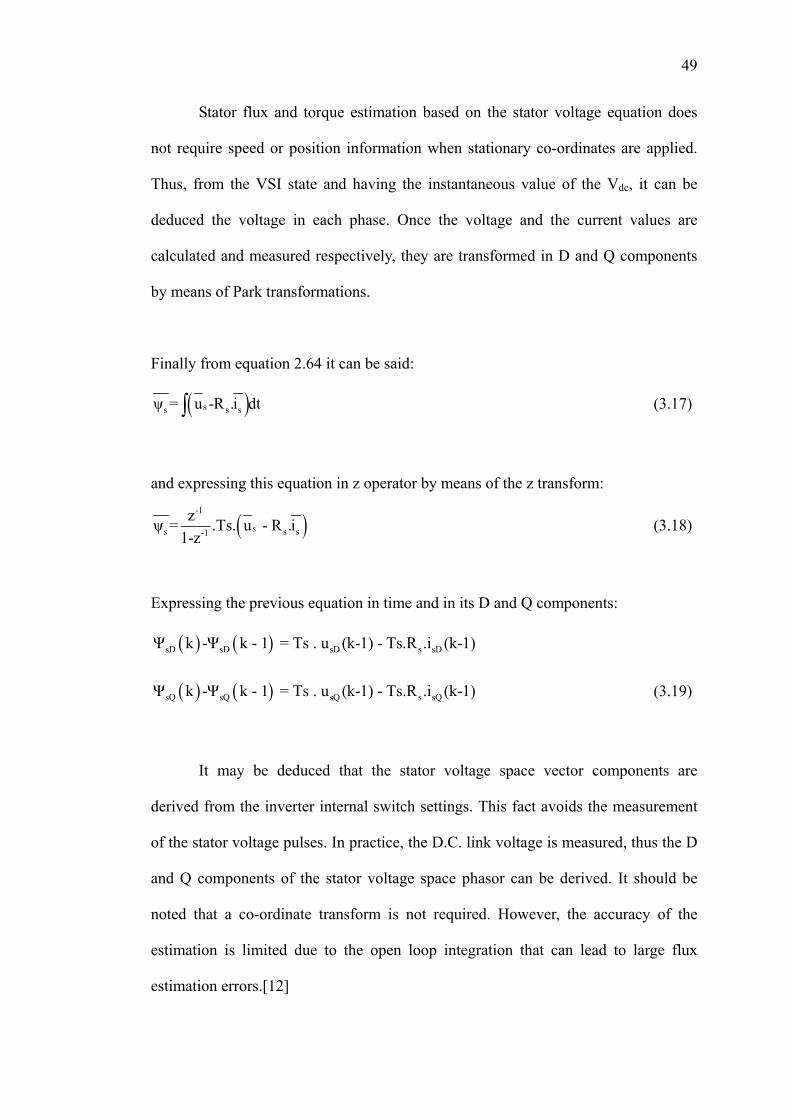
Finally from equation 2.64 it can be said:
( )ss sψ = u -R .i dt∫ s (3.17)
and expressing this equation in z operator by means of the z transform:
(-1
ss -1
zψ = .Ts. u - R .i1-z )s s (3.18)
Expressing the previous equation in time and in its D and Q components:
( ) ( )sD sD sD s sDΨ k -Ψ k - 1 = Ts . u (k-1) - Ts.R .i (k-1)
( ) ( )sQ sQ sQ s sQΨ k -Ψ k - 1 = Ts . u (k-1) - Ts.R .i (k-1) (3.19)
It may be deduced that the stator voltage space vector components are
derived from the inverter internal switch settings. This fact avoids the measurement
of the stator voltage pulses. In practice, the D.C. link voltage is measured, thus the D
and Q components of the stator voltage space phasor can be derived. It should be
noted that a co-ordinate transform is not required. However, the accuracy of the
estimation is limited due to the open loop integration that can lead to large flux
estimation errors.[12]
50
3.2.4 – Parameter detuning affects. [12][33]
Stator flux and torque estimators DTC based systems, shown in section
3.2.3.1 and 3.2.3.2.,depart from their ideal behavior when the motor model parameter
used are not different from the true motor model parameters. It can be proved that
estimators that use either position or speed have similar characteristics, which are
good enough, as long as the estimated parameters have an error lower than 10%.
However, the estimator that uses Vdc performs very poorly when just small errors of
its parameters are present. In further chapters will be used the estimator introduced in
section 3.2.3.1.
51
CHAPTER 4
DIRECT TORQUE CONTROL – SPACE VECTOR MODULATION (DTC – SVM)
4.1 INTRODUCTION
In principle classical DTC selects one of the six voltage vectors and two zero
voltage vectors generated by a VSI in order to keep stator flux and torque within the
limits of two hysteresis bands. The right application of this principle allows a
decoupled control of flux and torque without the need of coordinate transformations,
PWM pulse generation and current regulators.[11][9]
However, the presence of hysteresis controllers leads to a non-constant
switching frequency operation. The time discretization, due to the digital
52
implementation, and the limited number of available voltage vectors determine the
presence of current and torque ripples.[19] In order to overcome these problems,
different methods will been presented, allowing constant switching frequency
operation. They achieve a substantial reduction of current and torque ripples using, at
each cycle period, the calculation of the stator voltage space vector to exactly
compensate the flux and torque errors.
In order to apply this principle, the control system should be able to generate
the desired voltage vector, using the Space Vector Modulation technique (SVM).
These methods require more complex control schemes than basic DTC scheme and
present motor parameters dependence. The increased number of voltage vectors
allows the definition of more accurate switching tables in which the selection of the
voltage vectors is operated according to the rotor speed, the flux error and the torque
error, with no increase the complexity of classical DTC scheme.
The problem of switching table based DTC methods is that just after the
stator flux vector changes its position from one sector to another sector, there is no
active vector available that can assure an increase of stator flux. Therefore, at low
speed, especially with heavy load, stator flux droops systematically, causing the
stator flux trajectory to be nearly hexagonal and stator current distortions.[19]
Clearly the above DTC techniques present reciprocally advantages and disadvantages.
In this work a comparison of various direct torque control methodologies (Classical
DTC and SVM-DTC) will been made in order to evaluate the influence of the motor
operating condition on steady state performance.
53
4.2 VARIOUS DIRECT TORQUE CONTROL – SPACE VECTOR
MODULATION (DTC-SVM)
There are various types of direct torque control-space vector modulation
(DTC-SVM) schemes that have been proposed. Each scheme will perform the
different control technique but its aims are still similar which is to attain the constant
switching frequency and to reduce the torque ripple. The differences between various
DTC-SVM are on how the reference voltage is generated – the reference voltage is
then implemented using SVM. Space Vector Modulation is used to define the
inverter switching state or voltage vector positions different from six standard
positions.
4.2.1 DTC-SVM Scheme with Closed-Loop Torque Control
4.2.1.1 Basic Control Principle.
This method for direct torque control is based on load angle control strategy
and significantly overcomes the most important drawbacks of conventional direct
torque control. [16][21][9]A single space vector that represent the usual space vector
transformation apply to a three phase voltage system is defined as
54
( 2s a b
3u = u + u + u2
a a )c (4.1)
where 12 2
a j= − +3 , and, it is possible to obtain a simple equations set that describe
the AC machine dynamic behavior in a stator fixed coordinate system. These
equations are:
sss s
dψu =R i +dt
(4.2)
rr rr m
d0 = R .i - j.w +dtψψ (4.3)
ss msψ = L .i + L .ir (4.4)
rr mrψ = L .i + L .is (4.5)
The basic relation between torque and machine fluxes is:
re s r
s
k3T = - P [ψ xψ ]2 σL
re s r
s
k3T = - P ψ . ψ sin(δ)2 σL
(4.6)
where δ , known as load angle between stator and rotor fluxes as shown in Figure
4.1, kr =-Lm/Ls and σ =1-Lm2/ (Ls Lr). Based on 4.6, it is possible to achieve
machine speed and torque control directly by actuating over the load angle.
55
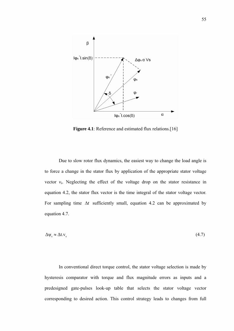
Figure 4.1: Reference and estimated flux relations.[16]
Due to slow rotor flux dynamics, the easiest way to change the load angle is
to force a change in the stator flux by application of the appropriate stator voltage
vector vs. Neglecting the effect of the voltage drop on the stator resistance in
equation 4.2, the stator flux vector is the time integral of the stator voltage vector.
For sampling time sufficiently small, equation 4.2 can be approximated by
equation 4.7.
t∆
s∆ψ ∆t.v≈ s (4.7)
In conventional direct torque control, the stator voltage selection is made by
hysteresis comparator with torque and flux magnitude errors as inputs and a
predesigned gate-pulses look-up table that selects the stator voltage vector
corresponding to desired action. This control strategy leads to changes from full
56
negative torque to full positive causing high torque ripple. The capability to actuate
on torque greatly depends on the electromotive force, s sω ϕ . This means that ripple
frequency varies with rotor speed obtaining variable switching frequency and a wide
spectrum for torque and stator current.
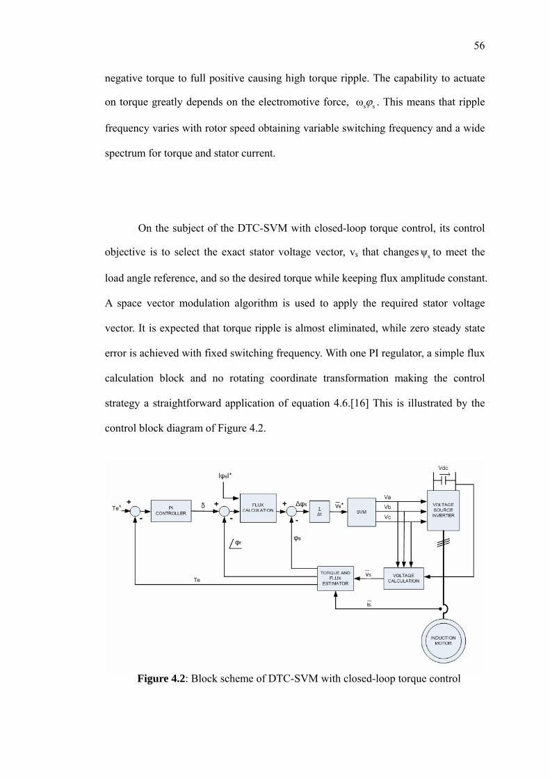
On the subject of the DTC-SVM with closed-loop torque control, its control
objective is to select the exact stator voltage vector, vs that changes to meet the
load angle reference, and so the desired torque while keeping flux amplitude constant.
A space vector modulation algorithm is used to apply the required stator voltage
vector. It is expected that torque ripple is almost eliminated, while zero steady state
error is achieved with fixed switching frequency. With one PI regulator, a simple flux
calculation block and no rotating coordinate transformation making the control
strategy a straightforward application of equation 4.6.[16] This is illustrated by the
control block diagram of Figure 4.2.
sψ
Figure 4.2: Block scheme of DTC-SVM with closed-loop torque control
57
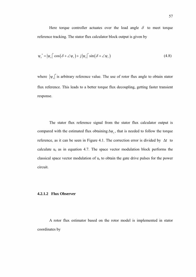
Here torque controller actuates over the load angle δ to meet torque
reference tracking. The stator flux calculator block output is given by
( ) (* **ψ ψ cos ψ ψ sin ψ )s s r sjδ= +∠ + + rδ ∠ (4.8)
where *ψs is arbitrary reference value. The use of rotor flux angle to obtain stator
flux reference. This leads to a better torque flux decoupling, getting faster transient
response.
The stator flux reference signal from the stator flux calculator output is
compared with the estimated flux obtaining sψ∆ , that is needed to follow the torque
reference, as it can be seen in Figure 4.1. The correction error is divided by t∆ to
calculate us as in equation 4.7. The space vector modulation block performs the
classical space vector modulation of us to obtain the gate drive pulses for the power
circuit.
4.2.1.2 Flux Observer
A rotor flux estimator based on the rotor model is implemented in stator
coordinates by
58
m s1ψ L i (1 ψ )
S
r mrr
jτ ωτ
⎡= − −⎢⎣∫S
r dt⎤⎥⎦
(4.9)
and the stator flux derived from
rs s
m
Lψ σL i + ψL
S S
s r= (4.10)
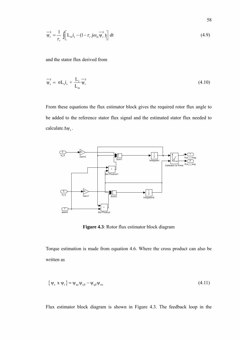
From these equations the flux estimator block gives the required rotor flux angle to
be added to the reference stator flux signal and the estimated stator flux needed to
calculate ψs∆ .
2flux_r_ang
1flux_r_mag
Sum2
Sum1
1s
Integrator2
1s
Integrator
-K-
Gain3
-K-
Gain1
Dot Product1
Dot Product
Cartesian to Polar
3is_q
2is_d
1speed
Figure 4.3: Rotor flux estimator block diagram
Torque estimation is made from equation 4.6. Where the cross product can also be
written as
{ }ψ x ψ ψ ψ ψ ψs r s r s rα β β= − α (4.11)
Flux estimator block diagram is shown in Figure 4.3. The feedback loop in the
59
integration of the rotor model can compensate for finite time disturbance in input is
and unknown initial conditions.
4.2.2 DTC-SVM Scheme With Closed-Loop Flux Control
4.2.2.1 Basic Control Principle
This control technique so-called stator flux vector control (SFVC) utilizes
the stator flux component as control variables. The scheme may be regarded as a
development of a direct torque control scheme, aimed at achieving constant
switching frequency operation. The voltage reference for space vector PWM is
calculated at each sampling period on the basis of the error between the reference
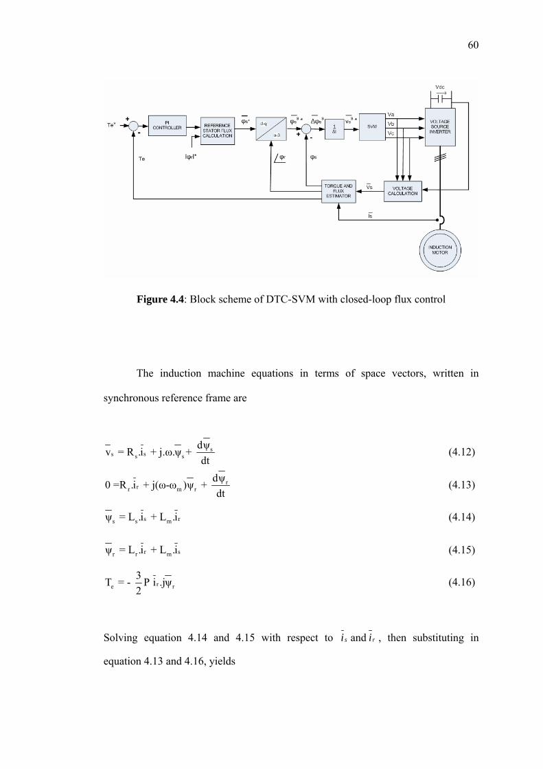
and the estimated stator flux vector.[20][9] Block diagram of the scheme based on
stator flux vector control is shown as Figure 4.4
60
Figure 4.4: Block scheme of DTC-SVM with closed-loop flux control
The induction machine equations in terms of space vectors, written in
synchronous reference frame are
sss s s
dψv = R .i + j.ω.ψ + dt
(4.12)
rrr m r
dψ0 =R .i + j(ω-ω )ψ + dt
(4.13)
ss msψ = L .i + L .ir (4.14)
rr mrψ = L .i + L .is (4.15)
re r3T = - P i .jψ2
(4.16)
Solving equation 4.14 and 4.15 with respect to si and ri , then substituting in
equation 4.13 and 4.16, yields
61
r m r rms
s r r
dψR L R0 = - ψ + + j(ω-ω ) ψ + σL L σL d
⎛ ⎞ ⎡ ⎤⎜ ⎟ ⎢ ⎥
⎣ ⎦⎝ ⎠r t
(4.17)
me s r
s r
L3T = P [ψ .jψ ]2 σL L
(4.18)
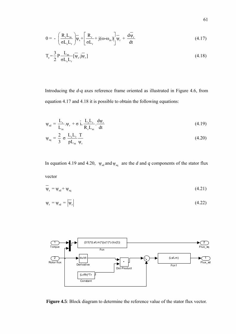
Introducing the d-q axes reference frame oriented as illustrated in Figure 4.6, from
equation 4.17 and 4.18 it is possible to obtain the following equations:
s s r rssd r
m r m
L L L dψψ = .ψ + σ i .L R L dt
(4.19)
s rsq
m r
L L2ψ = σ 3 pL ψ
T (4.20)
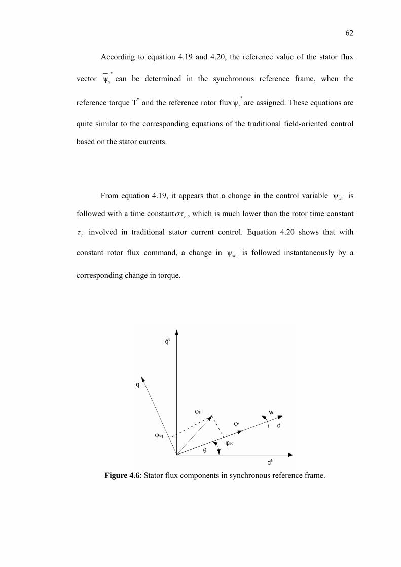
In equation 4.19 and 4.20, and are the d and q components of the stator flux
vector
sdψ sqψ
sd sqsψ = ψ + ψ (4.21)
r rd rψ = ψ = ψ (4.22)
2Flux_sq
1Flux_sd
(Ls/Lm)
Fcn1
(2/3)*(Ls/Lm)*((u(1)*Lr)/u(2))
Fcn
Dot Product
du/dt
Derivative
(Lr/Rr)*Tr
Constant
2Rotor flux
1Torque
Figure 4.5: Block diagram to determine the reference value of the stator flux vector.
62
According to equation 4.19 and 4.20, the reference value of the stator flux
vector *
sψ can be determined in the synchronous reference frame, when the
reference torque T* and the reference rotor flux*
rψ are assigned. These equations are
quite similar to the corresponding equations of the traditional field-oriented control
based on the stator currents.
From equation 4.19, it appears that a change in the control variable is
followed with a time constant
sdψ
rστ , which is much lower than the rotor time constant
rτ involved in traditional stator current control. Equation 4.20 shows that with
constant rotor flux command, a change in is followed instantaneously by a
corresponding change in torque.
sqψ
Figure 4.6: Stator flux components in synchronous reference frame.
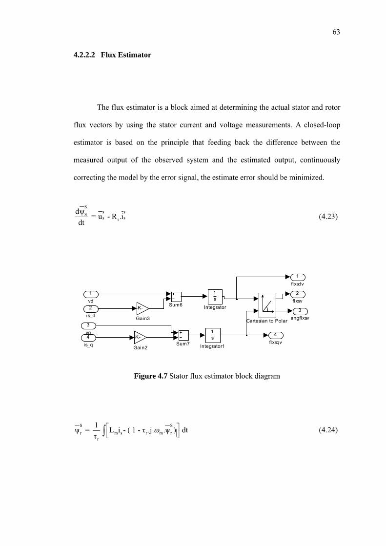
63
4.2.2.2 Flux Estimator
The flux estimator is a block aimed at determining the actual stator and rotor
flux vectors by using the stator current and voltage measurements. A closed-loop
estimator is based on the principle that feeding back the difference between the
measured output of the observed system and the estimated output, continuously
correcting the model by the error signal, the estimate error should be minimized.
S
sSss s
dψ = u - R .idt
s (4.23)
4flxsqv
3angflxsv
2flxsv
1flxsdv
Sum7
Sum6
1s
Integrator1
1s
Integrator-K-
Gain3
-K-
Gain2
Cartesian to Polar
4is_q
3vq
2is_d
1vd
Figure 4.7 Stator flux estimator block diagram
S
m s r mrr
1ψ = L i - ( 1 - τ .j. .ψ ) dtτ
ω⎡⎢⎣∫
S
r⎤⎥⎦
(4.24)
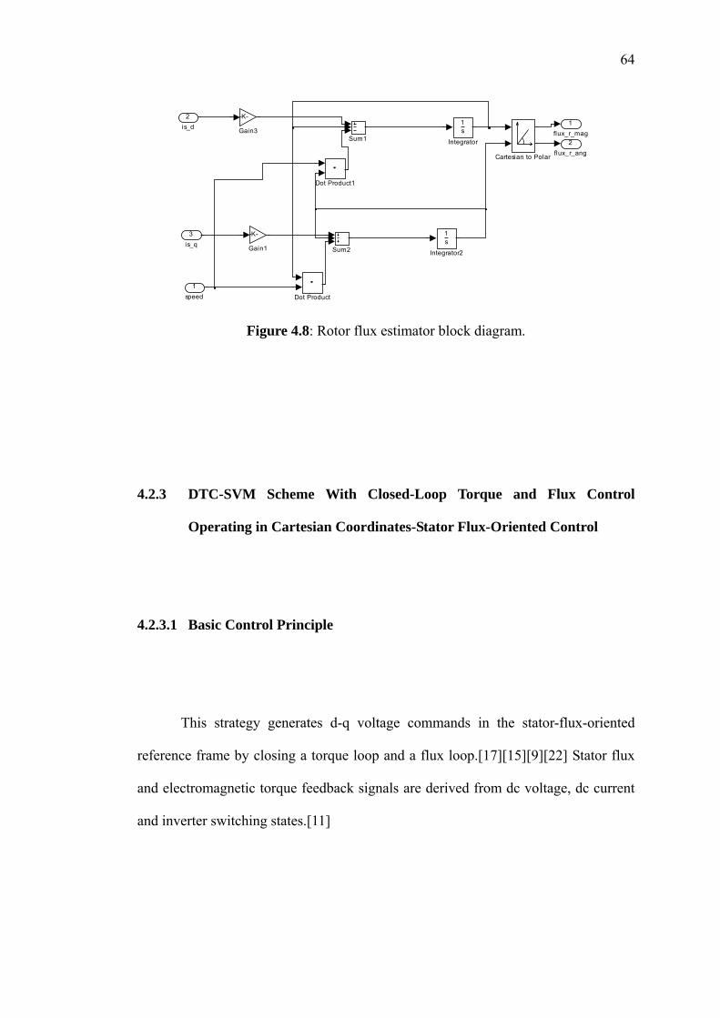
64
2flux_r_ang
1flux_r_mag
Sum2
Sum1
1s
Integrator2
1s
Integrator
-K-
Gain3
-K-
Gain1
Dot Product1
Dot Product
Cartesian to Polar
3is_q
2is_d
1speed
Figure 4.8: Rotor flux estimator block diagram.
4.2.3 DTC-SVM Scheme With Closed-Loop Torque and Flux Control
Operating in Cartesian Coordinates-Stator Flux-Oriented Control
4.2.3.1 Basic Control Principle
This strategy generates d-q voltage commands in the stator-flux-oriented
reference frame by closing a torque loop and a flux loop.[17][15][9][22] Stator flux
and electromagnetic torque feedback signals are derived from dc voltage, dc current
and inverter switching states.[11]
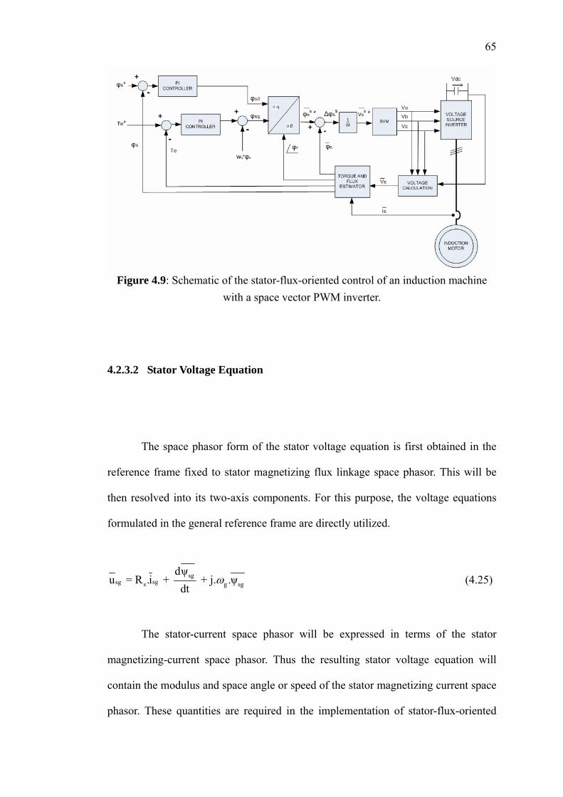
65
Figure 4.9: Schematic of the stator-flux-oriented control of an induction machine with a space vector PWM inverter.
4.2.3.2 Stator Voltage Equation
The space phasor form of the stator voltage equation is first obtained in the
reference frame fixed to stator magnetizing flux linkage space phasor. This will be
then resolved into its two-axis components. For this purpose, the voltage equations
formulated in the general reference frame are directly utilized.
sgsgsg s g
dψu = R .i + + j. .ψ
dtω sg (4.25)
The stator-current space phasor will be expressed in terms of the stator
magnetizing-current space phasor. Thus the resulting stator voltage equation will
contain the modulus and space angle or speed of the stator magnetizing current space
phasor. These quantities are required in the implementation of stator-flux-oriented
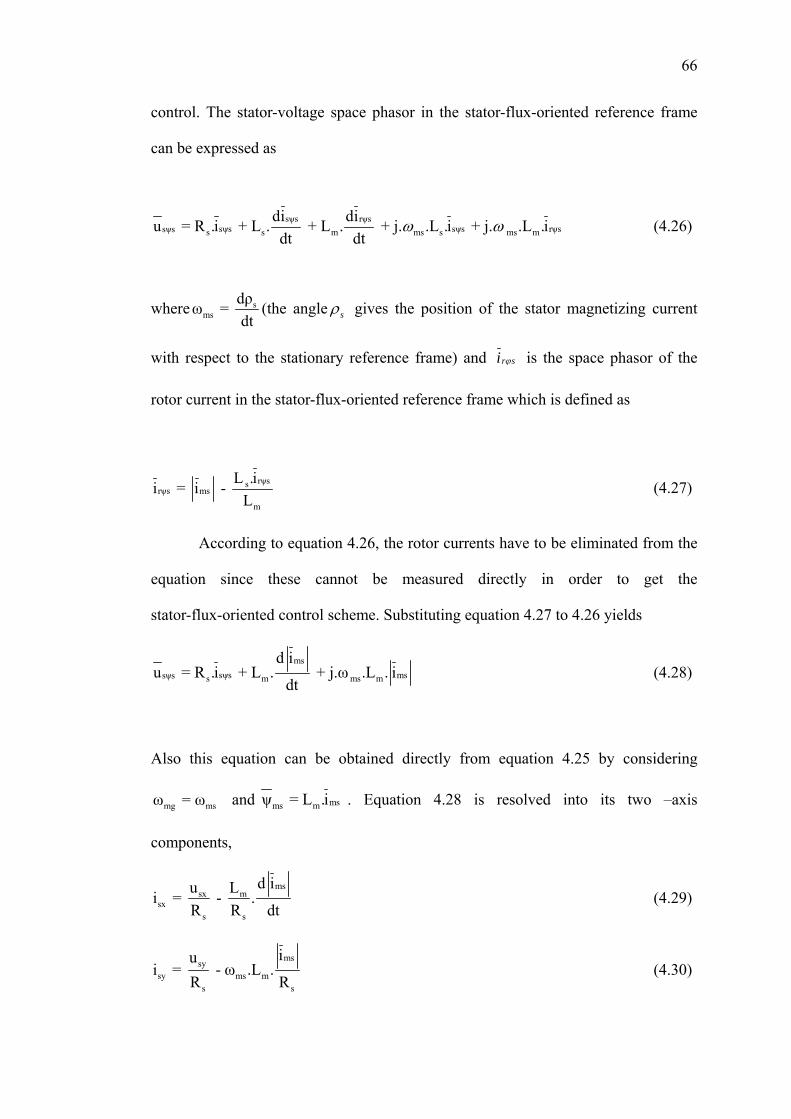
66
control. The stator-voltage space phasor in the stator-flux-oriented reference frame
can be expressed as
sψs rψssψs sψs rψssψs s s m ms s ms m
di diu = R .i + L . + L . + j. .L .i + j. .L .idt dt
ω ω (4.26)
where sms
dρω = dt
(the angle sρ gives the position of the stator magnetizing current
with respect to the stationary reference frame) and r si ϕ is the space phasor of the
rotor current in the stator-flux-oriented reference frame which is defined as
rψssrψs ms
m
L .ii = i - L
(4.27)
According to equation 4.26, the rotor currents have to be eliminated from the
equation since these cannot be measured directly in order to get the
stator-flux-oriented control scheme. Substituting equation 4.27 to 4.26 yields
mssψssψs s m ms m
d iu = R .i + L . + j.ω .L . i
dtms (4.28)
Also this equation can be obtained directly from equation 4.25 by considering
andmg msω = ω msmmsψ = L .i . Equation 4.28 is resolved into its two –axis
components,
mssx m
sxs s
d iu Li = - .R R dt
(4.29)
mssysy ms m
s s
iui = - ω .L .
R R (4.30)
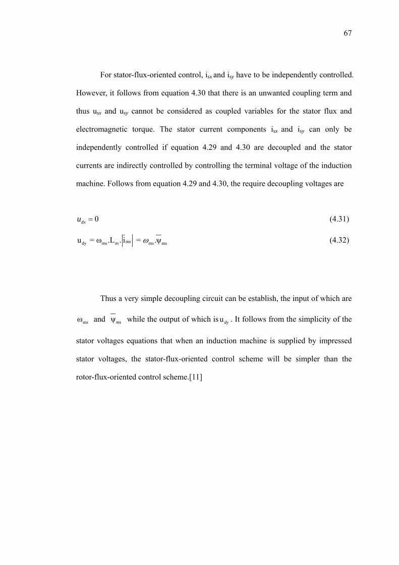
67
For stator-flux-oriented control, isx and isy have to be independently controlled.
However, it follows from equation 4.30 that there is an unwanted coupling term and
thus usx and usy cannot be considered as coupled variables for the stator flux and
electromagnetic torque. The stator current components isx and isy can only be
independently controlled if equation 4.29 and 4.30 are decoupled and the stator
currents are indirectly controlled by controlling the terminal voltage of the induction
machine. Follows from equation 4.29 and 4.30, the require decoupling voltages are
0dxu = (4.31)
msdy ms m ms msu = ω .L . i = .ψω (4.32)
Thus a very simple decoupling circuit can be establish, the input of which are
and msω ψms while the output of which is . It follows from the simplicity of the
stator voltages equations that when an induction machine is supplied by impressed
stator voltages, the stator-flux-oriented control scheme will be simpler than the
rotor-flux-oriented control scheme.[11]
udy
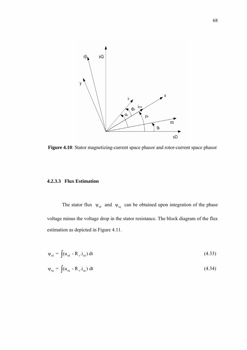
68
Figure 4.10: Stator magnetizing-current space phasor and rotor-current space phasor
4.2.3.3 Flux Estimation
The stator flux and can be obtained upon integration of the phase
voltage minus the voltage drop in the stator resistance. The block diagram of the flux
estimation as depicted in Figure 4.11.
sdψ sqψ
sd sd s sdψ = (u - R .i ) dt∫ (4.33)
sq sq s sqψ = (u - R .i ) dt∫ (4.34)
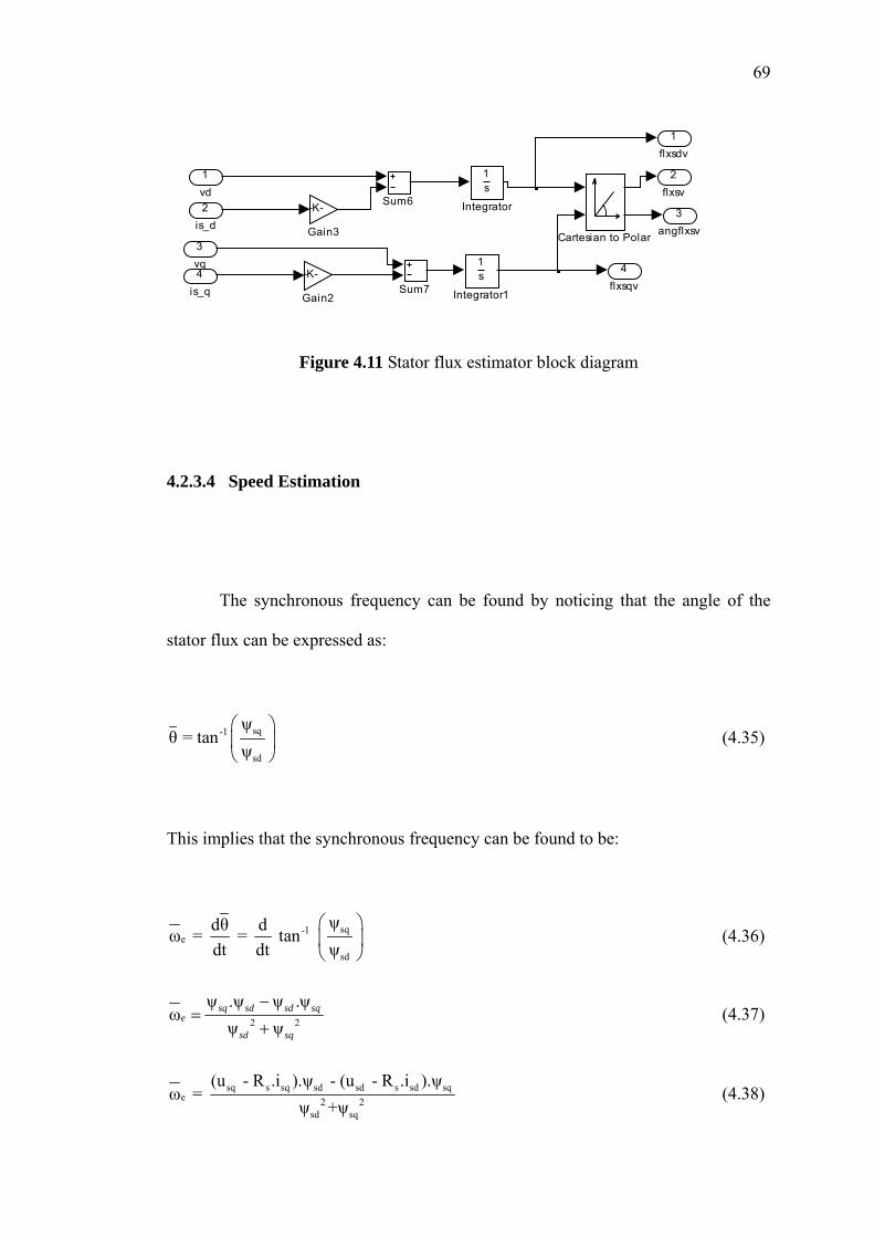
69
4flxsqv
3angflxsv
2flxsv
1flxsdv
Sum7
Sum6
1s
Integrator1
1s
Integrator-K-
Gain3
-K-
Gain2
Cartesian to Polar
4is_q
3vq
2is_d
1vd
Figure 4.11 Stator flux estimator block diagram
4.2.3.4 Speed Estimation
The synchronous frequency can be found by noticing that the angle of the
stator flux can be expressed as:
sq-1
sd
ψθ = tan
ψ⎛ ⎞⎜⎝ ⎠
⎟ (4.35)
This implies that the synchronous frequency can be found to be:
sq-1e
sd
ψdθ dω = = tan dt dt ψ
⎛ ⎞⎜⎝ ⎠
⎟ (4.36)
2 2
ψ .ψ ψ .ψω
ψ ψsq sd sd sq
e
sd sq
−=
+ (4.37)
sq s sq sd sd s sd sqe 2 2
sd sq
(u - R .i ).ψ - (u - R .i ).ψω =
ψ +ψ (4.38)
70
If rotor speed estimation is also desired, simple slip compensation can be derived
using the steady state torque-speed curve for the machine being used:
s s eω = K .T (4.39)
where K, is the slip frequency at rated torque and can be determined from the
nameplate of the machine.
The rotor speed is then given by
r eω = ω - ωs (4.40)
71
CHAPTER 5
ANALYSIS AND COMPARISON
5.1 INTRODUCTION
Convention DTC, DTC-SVM with closed loop-torque control, DTC-SVM
with closed loop-flux control and DTC-SVM with flux and torque control schemes
described in previous chapter have been simulated using Matlab/Simulink simulation
package. All simulations were performed using a model of the motors that have been
discussed in chapter two and the parameters of the motor are given in section 5.2.1.3
and the impact of different control strategies on the induction motor are compared to
each other and will be discussed in this chapter. The comparison will be focused on
the different methods applied to generate voltage reference of space vector PWM,
torque transient responses and flux trajectory for the each control schemes.
72
5.2 SIMULINK MODEL
5.2.1 Equation used in model
All the equations regarding to induction motor model have been expressed
in term of C language before it converted into S-function source - file compiled as a
MEX-file. Details of the C codes are given in the Appendix A.
5.2.1.1 Stator reference frame.
Stator and rotor fluxes can be expressed as follows:
(sD sD s sD1ψ = u - R .is
) (5.1)
(sQ sQ s sQ1ψ = u - R .is
) (5.2)
( ) (rd rd r rd m rq r rd m rq1 1ψ' = u' - R .i' - P.ω .ψ' = -R i' -P.ω ψ's s
) (5.3)
( ) (rq rq r rq m rd r rq m rd1 1ψ' = u' - R .i' - P.ω .ψ' = -R i' -P.ω ψ's s
) (5.4)
Stator and rotor currents can be expressed as follows:
rsD sD rd
x x
Li = ψ . - ψ' .L L
mL (5.5)
73
rsQ sQ rq
x x
Li = ψ . - ψ' .L L
mL (5.6)
s mrd rd sD
x x
L Li' = ψ' . - ψ .L L
(5.7)
s mrq rq sQ
x x
L Li' = ψ' . - ψ .L L
(5.8)
2x s rwhere L = L L - L m
5.2.1.2 The motion equation
The motion equation is defined as follows:
me L m
dωt - t = J + D.ωdt
(5.9)
where, te is the electromagnetic torque, tL is a load torque, J is the inertia of the rotor,
and finally the D is the damping constant.
By using the torque expression from the previous chapter, the motion
equation can be expressed as follows:
( ) ( )sD sQ sQ sD L mP.c ψ .i - ψ .i = t + ω D + J.s (5.10)
( )sD sQ sQ sD Lr
P.c ψ .i -ψ .i - tω =
D+Js (5.11)
where the torque constant take the values either 1 or 2/3.
74
5.2.1.3 Motor characteristics
For all simulation, the motor characteristics will be utilized as below:
Stator Resistance (ohm) = 5.5
Rotor Resistance (ohm) = 4.51
Stator Self Inductance (H) = 306.5e-3
Rotor Self Inductance (H) = 306.5e-3
Mutual Inductance (H) = 291.9e-3
No. of poles = 4
Moment of Inertia (kg.m^2) = 0.03
Load torque (Nm) = 1
While, the reference values for all cases were as follows:
• Torque reference value = 4 Nm
• Flux reference value = 1.2 Weber
• Torque hysteresis value = 2 Nm
• Flux hysteresis value = 0.02 Weber
• Sampling time, Ts = 0.00001 sec.
5.2.2 Conventional direct torque control
Principles of Direct Torque Control have been deeply explained in the chapter
two.[11][9] Using the SIMULINK/MATLAB, it will show that the method of
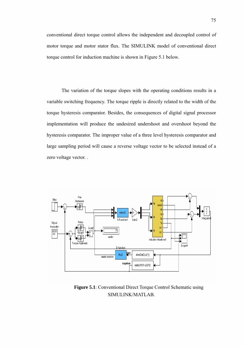
75
conventional direct torque control allows the independent and decoupled control of
motor torque and motor stator flux. The SIMULINK model of conventional direct
torque control for induction machine is shown in Figure 5.1 below.
The variation of the torque slopes with the operating conditions results in a
variable switching frequency. The torque ripple is directly related to the width of the
torque hysteresis comparator. Besides, the consequences of digital signal processor
implementation will produce the undesired undershoot and overshoot beyond the
hysteresis comparator. The improper value of a three level hysteresis comparator and
large sampling period will cause a reverse voltage vector to be selected instead of a
zero voltage vector. .
Figure 5.1: Conventional Direct Torque Control Schematic using SIMULINK/MATLAB.
76
5.2.3 DTC-SVM scheme with closed-loop torque control
Direct torque control based on load angle can result a very high quality
torque control without the need of tuning current controllers or using any co-ordinate
transformations. The use of DTC in conjunction with space vector modulation is
supposed to be one of the solutions to overcome the problems of convention direct
torque control-variable switching frequency, which depend on rotor, load and sample
frequency. Its main principles have been explained in the chapter five. Using the
SIMULINK/MATLAB blocks, it will be shown that the method of DTC-SVM allows
the torque response tracking the torque command at the input with its ripple
significantly reduced.
The SIMULINK model of DTC-SVM scheme with closed-loop torque
control for induction machine is shown in Figure 5.3 below. Obviously, from the
SIMULINK block diagram, this type of control technique is to present a very simple
one-step flux control algorithm and a straightforward controller that avoids
coordinate rotations and complex predictive controllers. Instead of induction motor
(IM), it can also be applied to the permanent magnet synchronous motor (PMSM).
[21][16][9]
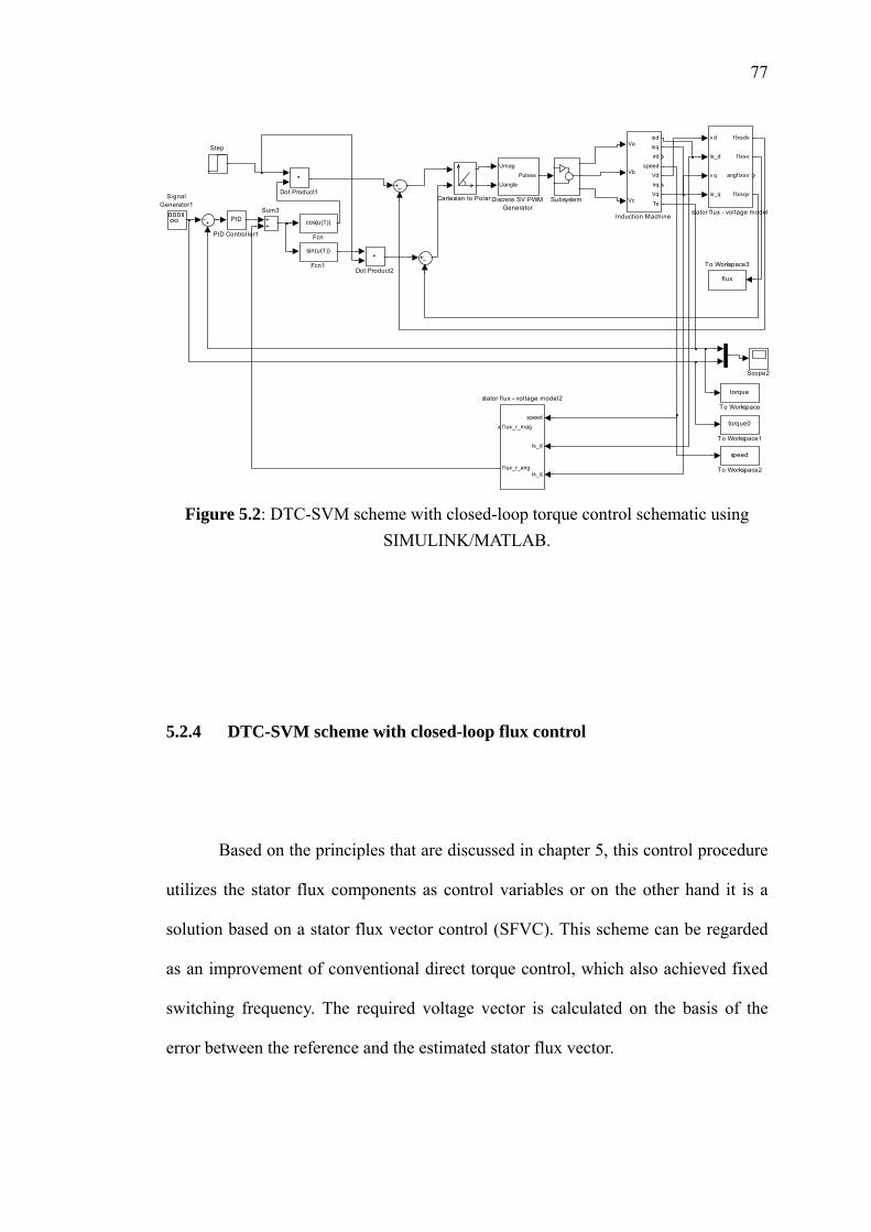
77
speed
is_d
is_q
f lux_r_mag
f lux_r_ang
stator flux - voltage model2
v d
is_d
v q
is_q
f lxsdv
f lxsv
angf lxsv
f lxsqv
stator flux - voltage model
flux
To Workspace3
speed
To Workspace2
torque0
To Workspace1
torque
To Workspace
Sum3
Subsystem
Step
SignalGenerator1
Scope2
PID
PID Control ler1
Va
Vb
Vc
isdisqird
speedVdirq
VqTe
Induction Machine
sin(u(1))
Fcn1
cos(u(1))
Fcn
Dot Product2
Dot Product1
Umag
UanglePulses
Discrete SV PWMGenerator
Cartesian to Polar
Figure 5.2: DTC-SVM scheme with closed-loop torque control schematic using SIMULINK/MATLAB.
5.2.4 DTC-SVM scheme with closed-loop flux control
Based on the principles that are discussed in chapter 5, this control procedure
utilizes the stator flux components as control variables or on the other hand it is a
solution based on a stator flux vector control (SFVC). This scheme can be regarded
as an improvement of conventional direct torque control, which also achieved fixed
switching frequency. The required voltage vector is calculated on the basis of the
error between the reference and the estimated stator flux vector.
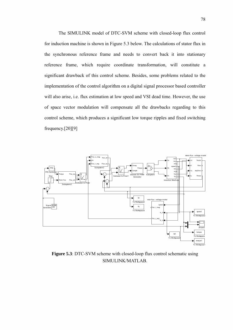
78
The SIMULINK model of DTC-SVM scheme with closed-loop flux control
for induction machine is shown in Figure 5.3 below. The calculations of stator flux in
the synchronous reference frame and needs to convert back it into stationary
reference frame, which require coordinate transformation, will constitute a
significant drawback of this control scheme. Besides, some problems related to the
implementation of the control algorithm on a digital signal processor based controller
will also arise, i.e. flux estimation at low speed and VSI dead time. However, the use
of space vector modulation will compensate all the drawbacks regarding to this
control scheme, which produces a significant low torque ripples and fixed switching
frequency.[20][9]
v d
id
v q
iq
f lxsdv
f lxsv
angf lxsv
f lxsqv
stator flux - voltage model
speed
is_d
is_q
f lux_r_mag
f lux_r_ang
rotor flux - voltage model
isd
To Workspace6
fq
To Workspace5
fd
To Workspace4
speed
To Workspace2
torque1
To Workspace1
torque
To Workspace
Flux_s_mag
phi
Flux_r_ang
f lux_sd
Flux_sq
Subsystem3
Torque
Rotor f lux
Flux_sq
Flux_sd
Subsystem2
SubsystemStep
Figure 5.3: DTC-SVM scheme with closed-loop flux control schematic using SIMULINK/MATLAB.
SignalGenerator
Scope2
PID
PID Controller1
Va
Vb
Vc
isd
isq
ird
speed
Vd
irq
Vq
Te
Induction Machine
Umag
Uangle
Pulses
Discrete SV PWMGeneratorCartesian to Polar1
Cartesian to Polar
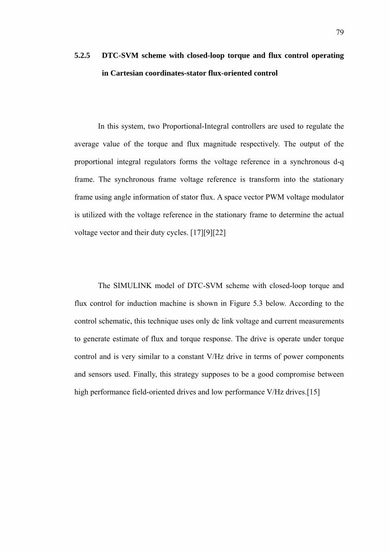
79
5.2.5 DTC-SVM scheme with closed-loop torque and flux control operating
in Cartesian coordinates-stator flux-oriented control
In this system, two Proportional-Integral controllers are used to regulate the
average value of the torque and flux magnitude respectively. The output of the
proportional integral regulators forms the voltage reference in a synchronous d-q
frame. The synchronous frame voltage reference is transform into the stationary
frame using angle information of stator flux. A space vector PWM voltage modulator
is utilized with the voltage reference in the stationary frame to determine the actual
voltage vector and their duty cycles. [17][9][22]
The SIMULINK model of DTC-SVM scheme with closed-loop torque and
flux control for induction machine is shown in Figure 5.3 below. According to the
control schematic, this technique uses only dc link voltage and current measurements
to generate estimate of flux and torque response. The drive is operate under torque
control and is very similar to a constant V/Hz drive in terms of power components
and sensors used. Finally, this strategy supposes to be a good compromise between
high performance field-oriented drives and low performance V/Hz drives.[15]
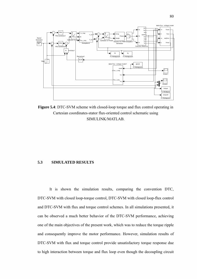
80
speed
is_d
is_q
f lux_r_mag
f lux_r_ang
stator flux - voltage model1
v d
id
v q
iq
f lxsdv
f lxsv
angf lxsv
f lxsqv
stator flux - voltage model
multiply1
fq
To Workspace5
fd
To Workspace4
speed
To Workspace2
torque0
To Workspace1
torque
To Workspace
V_s_mag
phi
Flux_r_ang
V_sd
V_sq
Subsystem2Subsystem
Step
SignalGenerator
Scope2
Scope1
PID
PID Controller2
PID
PID Controller1
Va
Vb
Vc
isd
isq
ird
speed
Vd
irq
Vq
Te
Induction Machine
Umag
Uangle
Pulses
Discrete SV PWMGenerator
du/dt
Derivative2
Cartesian to Polar2Cartesian to Polar1
Figure 5.4: DTC-SVM scheme with closed-loop torque and flux control operating in Cartesian coordinates-stator flux-oriented control schematic using
SIMULINK/MATLAB.
5.3 SIMULATED RESULTS
It is shown the simulation results, comparing the convention DTC,
DTC-SVM with closed loop-torque control, DTC-SVM with closed loop-flux control
and DTC-SVM with flux and torque control schemes. In all simulations presented, it
can be observed a much better behavior of the DTC-SVM performance, achieving
one of the main objectives of the present work, which was to reduce the torque ripple
and consequently improve the motor performance. However, simulation results of
DTC-SVM with flux and torque control provide unsatisfactory torque response due
to high interaction between torque and flux loop even though the decoupling circuit
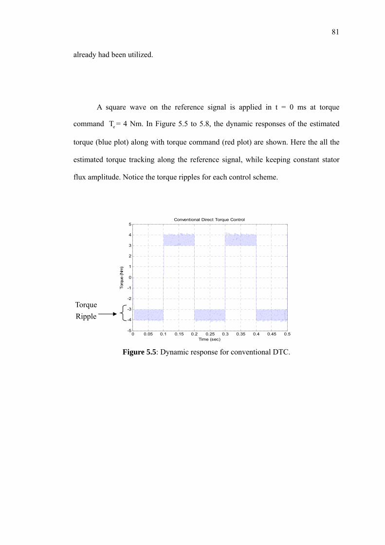
81
already had been utilized.
A square wave on the reference signal is applied in t = 0 ms at torque
command = 4 Nm. In Figure 5.5 to 5.8, the dynamic responses of the estimated
torque (blue plot) along with torque command (red plot) are shown. Here the all the
estimated torque tracking along the reference signal, while keeping constant stator
flux amplitude. Notice the torque ripples for each control scheme.
eT
0 0.05 0.1 0.15 0.2 0.25 0.3 0.35 0.4 0.45 0.5-5
-4
-3
-2
-1
0
1
2
3
4
5Conventional Direct Torque Control
Time (sec)
Torq
ue (N
m)
Torque Ripple
Figure 5.5: Dynamic response for conventional DTC.
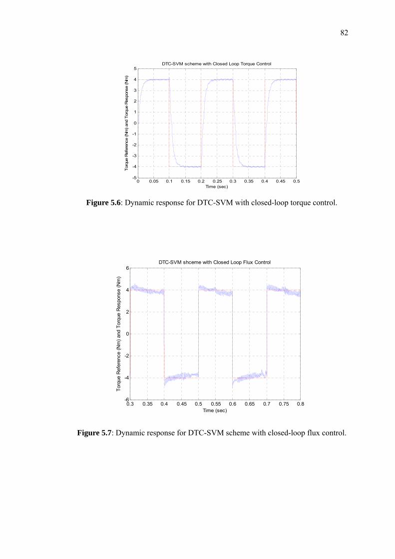
82
0 0.05 0.1 0.15 0.2 0.
25 0.3 0.35 0.4 0.45 0.5
-5
-4
-3
-2
-1
0
1
2
3
4
5
Time (sec)
Torq
ue R
efer
ence
(Nm
) and
Tor
que
Res
pons
e (N
m)
DTC-SVM scheme with Closed Loop Torque Control
Figure 5.6: Dynamic response for DTC-SVM with closed-loop torque control.
0.3 0.35 0.4 0.45 0.5 0.55 0.6 0.65 0.7 0.75 0.8-6
-4
-2
0
2
4
6
Time (sec)
Torq
ue R
efer
ence
(Nm
) and
Tor
que
Res
pons
e (N
m)
DTC-SVM shceme with Closed Loop Flux Control
Figure 5.7: Dynamic response for DTC-SVM scheme with closed-loop flux control.
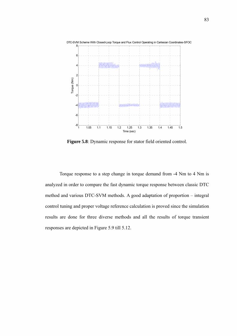
83
1 1.05 1.1 1.15 1.2 1.25 1.3 1.35 1.4 1.45 1.5-8
-6
-4
-2
0
2
4
6
8
Time (sec)
Torq
ue (N
m)
DTC-SVM Scheme With Closed-Loop Torque and Flux Control Operating in Cartesian Coordinates-SFOC
Figure 5.8: Dynamic response for stator field oriented control.
Torque response to a step change in torque demand from -4 Nm to 4 Nm is
analyzed in order to compare the fast dynamic torque response between classic DTC
method and various DTC-SVM methods. A good adaptation of proportion – integral
control tuning and proper voltage reference calculation is proved since the simulation
results are done for three diverse methods and all the results of torque transient
responses are depicted in Figure 5.9 till 5.12.
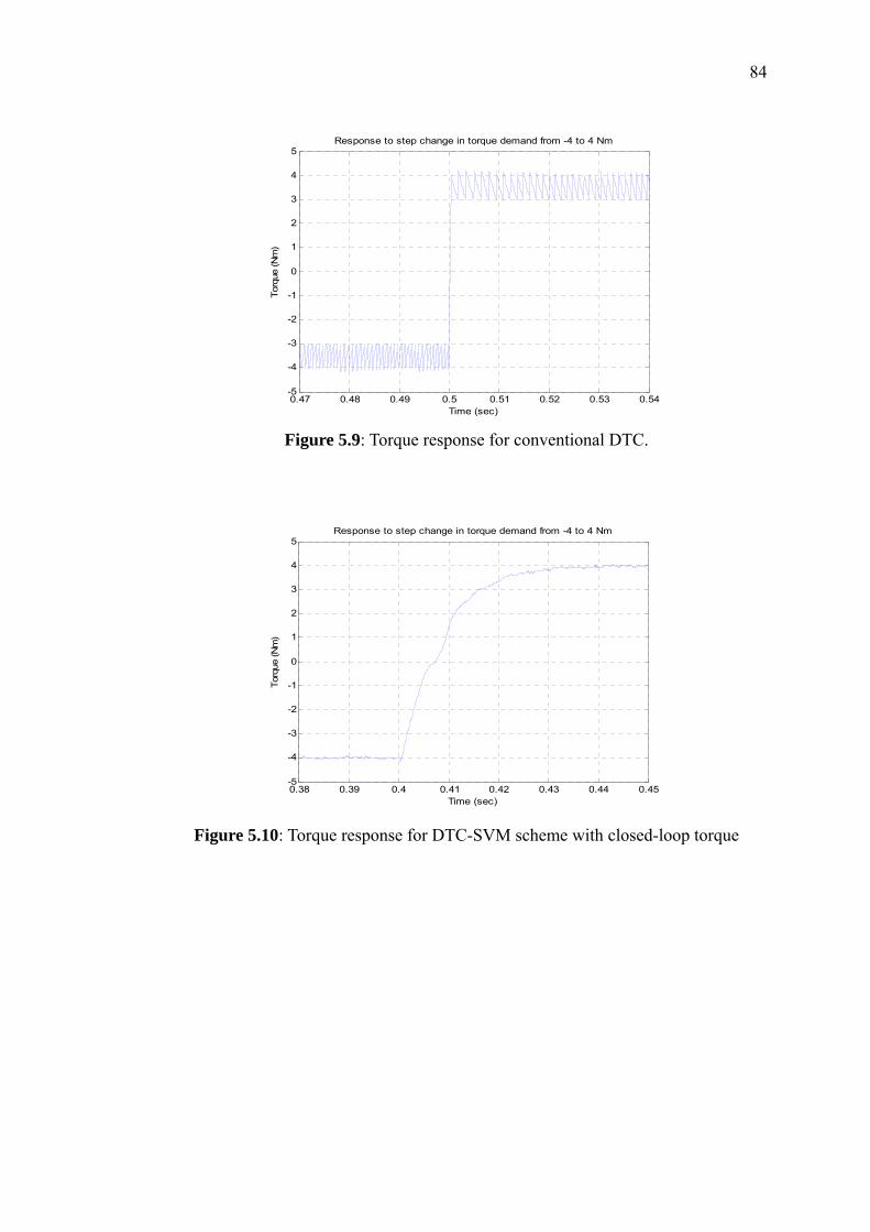
84
0.47 0.48 0.49 0.5 0.51 0.52 0.53 0.54-5
-4
-3
-2
-1
0
1
2
3
4
5
Time (sec)
Torq
ue (N
m)
Response to step change in torque demand from -4 to 4 Nm
Figure 5.9: Torque response for conventional DTC.
0.38 0.39 0.4 0.41 0.42 0.43 0.44 0.45-5
-4
-3
-2
-1
0
1
2
3
4
5
Time (sec)
Torq
ue (N
m)
Response to step change in torque demand from -4 to 4 Nm
Figure 5.10: Torque response for DTC-SVM scheme with closed-loop torque
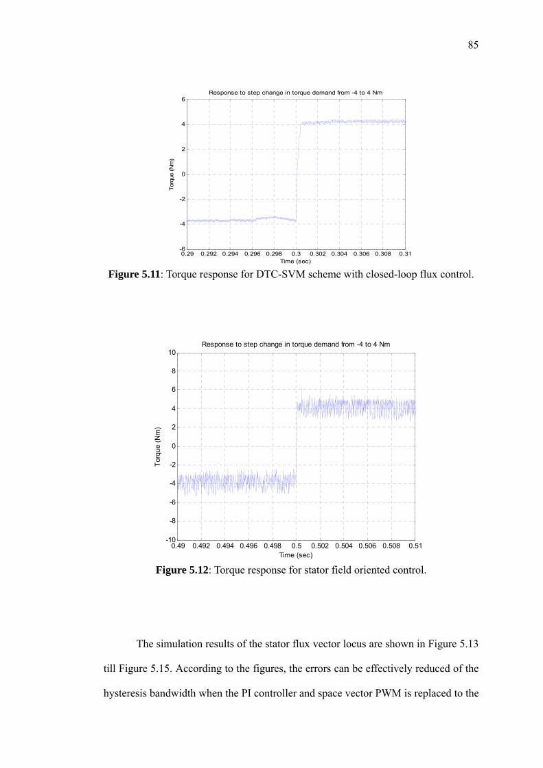
85
0.29 0.292 0.294 0.296 0.298 0.3 0.302 0.304 0.306 0.308 0.31-6
-4
-2
0
2
4
6Response to step change in torque demand from -4 to 4 Nm
Time (sec)
Torq
ue (N
m)
Figure 5.11: Torque response for DTC-SVM scheme with closed-loop flux control.
0.49 0.492 0.494 0.496 0.498 0.5 0.502 0.504 0.506 0.508 0.51-10
-8
-6
-4
-2
0
2
4
6
8
10
Time (sec)
Torq
ue (N
m)
Response to step change in torque demand from -4 to 4 Nm
Figure 5.12: Torque response for stator field oriented control.
The simulation results of the stator flux vector locus are shown in Figure 5.13
till Figure 5.15. According to the figures, the errors can be effectively reduced of the
hysteresis bandwidth when the PI controller and space vector PWM is replaced to the
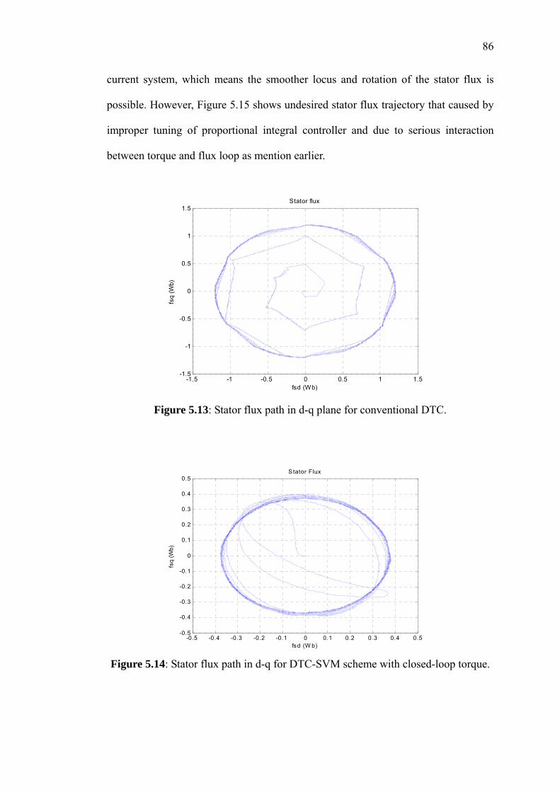
86
current system, which means the smoother locus and rotation of the stator flux is
possible. However, Figure 5.15 shows undesired stator flux trajectory that caused by
improper tuning of proportional integral controller and due to serious interaction
between torque and flux loop as mention earlier.
-1.5 -1 -0.5 0 0.5 1 1.5-1.5
-1
-0.5
0
0.5
1
1.5Stator flux
fsd (Wb)
fsq
(Wb)
Figure 5.13: Stator flux path in d-q plane for conventional DTC.
-0.5 -0.4 -0.3 -0.2 -0.1 0 0.1 0.2 0.3 0.4 0.5-0.5
-0.4
-0.3
-0.2
-0.1
0
0.1
0.2
0.3
0.4
0.5S tator Flux
fsd (W b)
fsq
(Wb)
Figure 5.14: Stator flux path in d-q for DTC-SVM scheme with closed-loop torque.
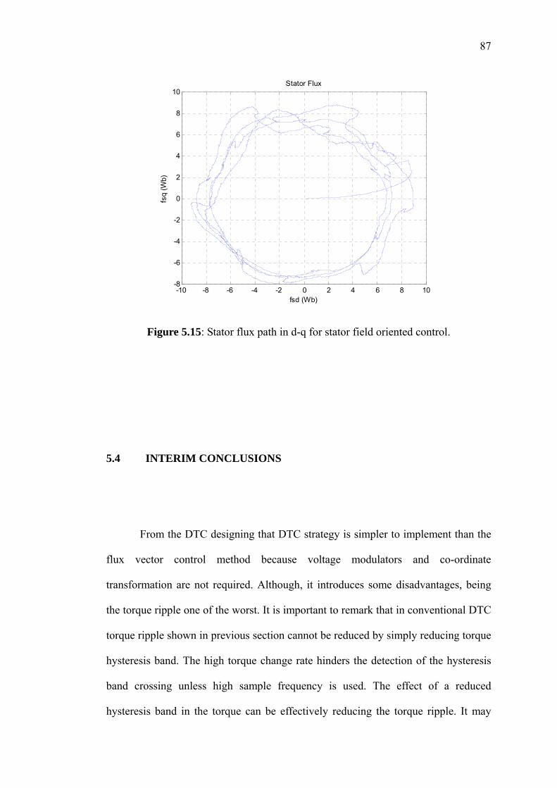
87
-10 -8 -6 -4 -2 0 2 4 6 8 10-8
-6
-4
-2
0
2
4
6
8
10
fsd (Wb)
fsq
(Wb)
Stator Flux
Figure 5.15: Stator flux path in d-q for stator field oriented control.
5.4 INTERIM CONCLUSIONS
From the DTC designing that DTC strategy is simpler to implement than the
flux vector control method because voltage modulators and co-ordinate
transformation are not required. Although, it introduces some disadvantages, being
the torque ripple one of the worst. It is important to remark that in conventional DTC
torque ripple shown in previous section cannot be reduced by simply reducing torque
hysteresis band. The high torque change rate hinders the detection of the hysteresis
band crossing unless high sample frequency is used. The effect of a reduced
hysteresis band in the torque can be effectively reducing the torque ripple. It may
88
conclude then, that the only way to improve classic DTC performance is to increase
sampling frequency, this is normally not possible due to constraints on the switching
frequency and minimum computational time requirement.
By using the predictive one, supposed the classical DTC drawbacks will be
overcoming and consequently improve the DTC performance. The calculation of the
proper voltage reference that needs to feed into space vector PWM is required as
discussed in chapter 5. The fixed switching frequency methods require a fast
processor for realization since the duty cycles or voltage vectors need to be
calculated for every sampling period, particularly when a small sampling period is
required for substantially small torque ripple.
The scheme of DTC-SVM with closed-loop torque control and
field-oriented control share the similar dynamic responses and speed reference
tracking. Basically, the proposed of this control scheme is based on few induction
motor equations. The conventional DTC shows high torque and flux ripples while
this method reduces torque and flux ripple significantly. It is clearly demonstrated
that the use of DTC in conjunction with SVM greatly improves torque performance.
The dynamic behavior of the stator flux vector control (SFVC) scheme has
been verified during a stating transient. A step torque command of 4 Nm has been
applied to the drive system. Figure 3.0 shows the estimated values of torque while on
figure 3.1 is the command torque waveform. The generated torque decreases
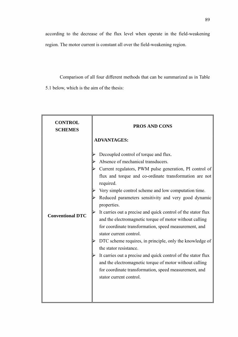
89
according to the decrease of the flux level when operate in the field-weakening
region. The motor current is constant all over the field-weakening region.
Comparison of all four different methods that can be summarized as in Table
5.1 below, which is the aim of the thesis:
CONTROL SCHEMES
PROS AND CONS
Conventional DTC
ADVANTAGES: Decoupled control of torque and flux. Absence of mechanical transducers. Current regulators, PWM pulse generation, PI control of
flux and torque and co-ordinate transformation are not required.
Very simple control scheme and low computation time. Reduced parameters sensitivity and very good dynamic
properties. It carries out a precise and quick control of the stator flux
and the electromagnetic torque of motor without calling for coordinate transformation, speed measurement, and stator current control.
DTC scheme requires, in principle, only the knowledge of the stator resistance.
It carries out a precise and quick control of the stator flux and the electromagnetic torque of motor without calling for coordinate transformation, speed measurement, and stator current control.
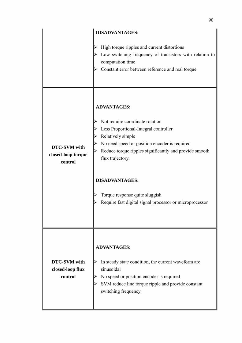
90
DISADVANTAGES: High torque ripples and current distortions Low switching frequency of transistors with relation to
computation time Constant error between reference and real torque
DTC-SVM with closed-loop torque
control
ADVANTAGES: Not require coordinate rotation Less Proportional-Integral controller Relatively simple No need speed or position encoder is required Reduce torque ripples significantly and provide smooth
flux trajectory. DISADVANTAGES: Torque response quite sluggish Require fast digital signal processor or microprocessor
DTC-SVM with closed-loop flux
control
ADVANTAGES: In steady state condition, the current waveform are
sinusoidal No speed or position encoder is required SVM reduce line torque ripple and provide constant
switching frequency
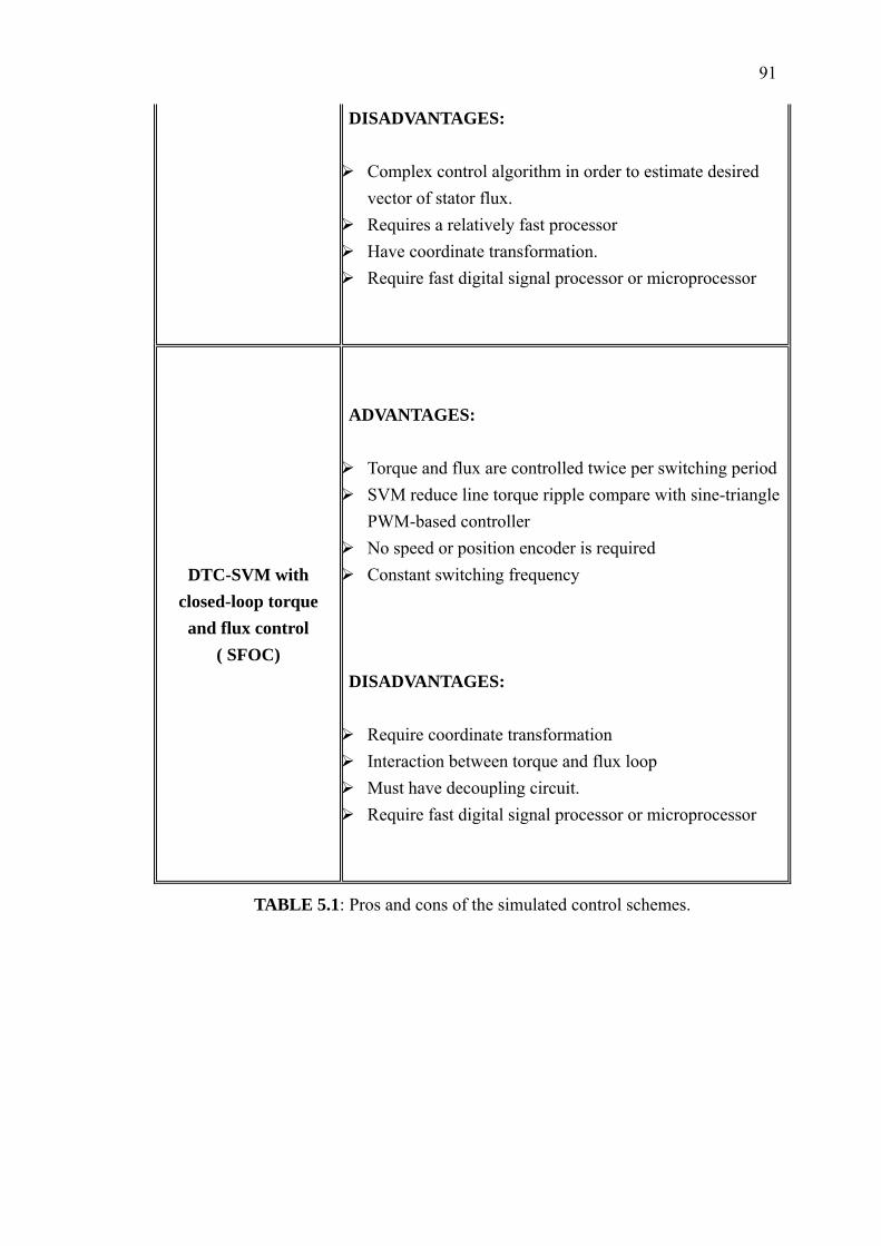
91
DISADVANTAGES: Complex control algorithm in order to estimate desired
vector of stator flux. Requires a relatively fast processor Have coordinate transformation. Require fast digital signal processor or microprocessor
DTC-SVM with closed-loop torque
and flux control ( SFOC)
ADVANTAGES: Torque and flux are controlled twice per switching period SVM reduce line torque ripple compare with sine-triangle
PWM-based controller No speed or position encoder is required Constant switching frequency
DISADVANTAGES: Require coordinate transformation Interaction between torque and flux loop Must have decoupling circuit. Require fast digital signal processor or microprocessor
TABLE 5.1: Pros and cons of the simulated control schemes.
92
CHAPTER 6
CONCLUSION AND RECOMMENDATION FOR FUTURE
WORK
6.1 CONCLUSION
Direct Torque Control is supposed to be one of the best controllers for
driving any induction motor. Its principles and basic concepts have been introduced
and thoroughly explained. It is also demonstrated in the thesis that the method of
direct torque control also allows the decoupled control of motor torque and motor
stator flux. According to the analysis, the DTC strategy is simpler to implement than
the flux vector control method because it does not require voltage modulators, and
co-ordinate transformations. However, it introduces undesired torque ripple. Several
different methods for improving classical DTC can be described as below:
The search of a better look up table. Following some research that have been
93
done in this field, optimum look up table cannot be remarkably improved the
DTC performance. Nevertheless, some improvement can be achieved and it
will give the fundamental idea for the development of ideal controller.
Implies the predictive method, which requires the usage of space vector
modulation and the calculation of the proper voltage reference. This method
exists in various control manners such as torque or flux only control and its
aims are to overcome the drawbacks of conventional DTC. Therefore, the
present thesis has been focused on that.
The application of the fuzzy logic for implementing a simple modulation
between the selected active state and a zero state is another method to
improve conventional DTC.[33]
Another method that looks promising is the regulation of the stator flux
reference value. This method can be applied in any motor drive and instead of
reduces the torque ripple; it also reduces the power reactive consumption
taken from main supply.
After all the research done, this thesis is focused on the analysis of several
DTC-SVM control schemes. Space vector modulation technique is used to synthesize
the desired stator voltage. In other words, SVM technique used the voltage reference
to determine the appropriate controlled duty cycle for every sampling period in order
to compensate the torque and stator flux vector error. It has been deeply described
and justified that the voltage reference can be determined in various ways and
making emphasis on its inputs had to be the torque errors and flux locus.
Simulation results show the validity of the various DTC-SVM techniques
94
not only achieve a considerable reduction in torque and flux ripple, but also provide
constant inverter switching frequency and dramatically increase the inverter
switching frequency without requiring any high frequency dither signal. One of DTC
in conjunction with space vector modulation already been proved that its not only to
produced a powerful alternative to overcome the well known drawbacks of the
original DTC solution, but also perform a simple control method and easy to
implement. [23][24]
6.2 RECOMMENDATION FOR FUTURE WORK
All the further work is summarized as follows :-
Comparative study of various DTC-SVM schemes for Induction Motor
experimentally. Experimental results will show the validity of the entire
research.
Simulation and experimental test of various DTC-SVM techniques applied to
the Permanent Magnet Synchronous Motor (PMSM).
Develop a fuzzy controller to achieve a better performance. This fuzzy
controller should take into account the following ideas:
Develop a completely auto adaptive controller.
The controller must be adaptive to any motor.
Try to overcome the electrical noises, which appear in any power drive.
Study the torque ripple reduction not only with fuzzy modulators but also

95
with multilevel converter.
Find optimum controllers, not only for torque ripple reductions, but also for
improving energy utilizations.[33]
96
REFERENCES
1. Peter Vas, “Electrical machines and drives: A space-vector theory
approach”, Oxford University Press 1992.
2. Mohan, Undeland, Robbins. “Power Electronics” Wiley. Second edition.
1989.
3. Leonhard, W. “Control of Electrical Drives” Springler-Verlag, 1990.
4. Ludtke, I.; Jayne M.G. “ A comparative study of high performance speed
control strategies for voltage sourced PWM inverter fed induction motor
drives”, Seventh International Conference on Electrical Machines and
Drives, 11-13 September 1995, University of Durham, UK.
5. Bose, B. K. “Power Electronics and AC Drives” Prentice Hall, 1986.
6. Romeral, J. L.;”Optimization of Digital Control for AC Motor”
Doctorial Thesis, University de Catalunya, June 1995.
7. N. Mohan, Advanced Electric Drives. Minneapolis, MN: MNPERE,
2001.
8. Yamamura, S.; “AC Motor for high-performance applications. Analysis
and Control” Ed Marcel Dekka, Inc. 1986.
97
9. Giuseppe S. Buja, and Marian P. Kazmierkowski, “Direct Torque
Control of PWM Inverter-Fed AC Motors - A Survey,” IEEE Trans On
Ins Electronics, 50(4) 744-757 August 2004
10. Bedford, D.;” Adaptive Vector Control of Asynchronous Induction
Motor” Doctorial Thesis, University de Catalunya, October 1995.
11. Peter Vas, “Sensor less Vector and Direct Torque Control”, Oxford
University Press, London, 1998.
12. Ludtke, I; “The Direct Torque Control of Induction Motors” Thesis
Department of Electronics and Information Technology, University of
Glamorgan, May 1998.
13. Boldeea, I; “Nasar, S.A. “Vector Control of AC Drives “CRC Press Inc.,
1992.
14. Takahashi, I. and Ohimori, Y. “ High Performance Direct Torque Control
of an Induction Motor” IEEE Trans. Industry applications, Vol. 25,
257-264, March 1989.
15. X. Xue, X. Xu, T. G. Habetler, and D. M. Divan, “A low cost stator flux
oriented voltage source variable speed drive,” in Conf. Rec. IEEE-IAS
Annual Meeting, vol. 1, 1990, pp. 410–415.
98
16. J. Rodriquez, Jorge Pontt, C Selva and H. Miranda, “A Novel Direct
Torque Control Scheme for Induction Machines With Space Vector
Modulation,” IEEE Trans Power Electronic pp 1392-1397, 2004.
17. Yen-Shin Lai and Jian-Ho Chen,” A New Approach to Direct Torque
Control of Induction Motor Drives for Constant Inverter Switching
Frequency and Torque Ripple Reduction” IEEE Trans. on Energy
Conversion, Vol. 2: 220-227 September 2001
18. J. Rodriquez, Jorge Pontt, C Selva and H. Miranda, “ Simple direct
torque control of induction machines using space vector modulation”
Electronics Letter, Volume 40, No. 7.
19. P. Marino, M. D’Incecco and N. Visciano,” A Comparison of Direct
Torque Control Methodologies for Induction Motor,” IEEE Porto Power
Tech. Conference, September 2001, Portugal.
20. D. Casadei, G Serra, A. Tani, L Zaari and F. Profumo, ”Performance
Analysis of a Speed-Sensor less Induction Motor Drive Based on a
Constant-Switching-Frequency DTC Scheme,” IEEE Trans. On Ins.
Application, 39(2) 476-484 March/April 2003.
21. N. R. N. Idris and A. H. Yatim, “Reduced torque ripple and constant
torque switching frequency strategy for induction motors,” in Proc.
IEEE APEC’00, 2000, pp. 154–161.
99
22. T. G. Habetler, F. Profumo, M. Pastorelli, and L. M. Tolbert, “Direct
torque control of induction motor using space vector modulation,” IEEE
Trans. Ind. Application., vol. 28, pp. 1045–1053, Sept. /Oct. 1992.
23. Isao Takahashi and Toshihiko Noguchi,” Take a Look Back upon the
Past Decade of Direct Torque Control,” 546-551, 1997.
24. Toshihiko Noguchi, Masaki Yamamoto, Isao Takahashi,” Enlarging
Switching Frequency in Direct Torque-Controlled Inverter by Means of
Dithering”, IEEE Trans. On Ind. Application, vol. 35, pp. 1358–1366,
Nov. /Dec. 1999.
25. I. Takahashi and T. Noguchi, “A new quick-response and high efficiency
control strategy of an induction machine,” IEEE Trans. Ind. Application,
vol. IA-22, pp. 820–827, Sept. /Oct. 1986.
26. F. Blaschke, “The principle of field-orientation as applied to the
transvector closed-loop control system for rotating-field machines,”
Siemens Rev., vol. 34, pp. 217–220, 1972.
27. M. Depenbrock, “Direct self control of inverter-fed induction
machines,” IEEE Trans. Power Electron., vol. 3, pp. 420–429, Oct.1988.
28. Keliang Zhou and Danwei Wang,” Relationship between Space Vector
Modulation and Three-Phase Carrier-Based PWM: A Comprehensive
Analysis,” IEEE Trans. On Ins Electronics, 49(1), 186-196 August 2004
100
29. Dr. Nik Rumzi Nik Idris, Notes of Direct Torque Control of Induction
Machine.
30. J.C Trounce, S.D Round and R.M Duke, “ Comparison By Simulation of
Three-Level Induction Motor Torque Control Scheme For Electric
Vehicle Application,”
31. L. Xu and M. Fu, “A novel sensorless control technique for permanent
magnet synchronous motors (PMSM) using digital signal processor
(DSP),” in Proc. NEACON’97, Dayton, OH, July 14–17, 1997, pp.
403–406.
32. Implementation of a Direct Torque Control Algorithm for Induction
Motor Based on Discrete Space Vector Modulation,” IEEE Trans On
Power Electronics, 15 (4) 769-776 July 2000
33. Arias Pujol, “Improvements in direct torque control of induction
motors,” Master Thesis, March 2001
34. M.P. Kazmierkowski and A.B. Kasprowicz, “Improved direct torque and
flux control of PWM inverter-fed induction motor drives”, IEEE Trans.
Ind. Electronics, Vol. 42, No. 4 Aug 1995.
35. Bingsen Wang,” Study on an Induction Motor Excited by PWM
Voltage-Source Inverter via Simulation,”2004
101
APPENDIX A
#define S_FUNCTION_NAME imch /* Input Arguments */ /* * Need to include simstruc.h for the definition of the SimStruct and * its associated macro definitions. */ /* #include "tmwtypes.h" */ #include "tmwtypes.h" #include "simstruc.h" #define Rs ssGetArg(S,0) #define Rr ssGetArg(S,1) #define Ls ssGetArg(S,2) #define Lr ssGetArg(S,3) #define Lm ssGetArg(S,4) #define pole ssGetArg(S,5) /*====================* * S-function methods * *====================*/ /* Function: mdlInitializeSizes =============================================== * Abstract: * * The sizes information is used by SIMULINK to determine the S-function * block's characteristics (number of inputs, outputs, states, etc.). * */ static void mdlInitializeSizes(SimStruct *S) {
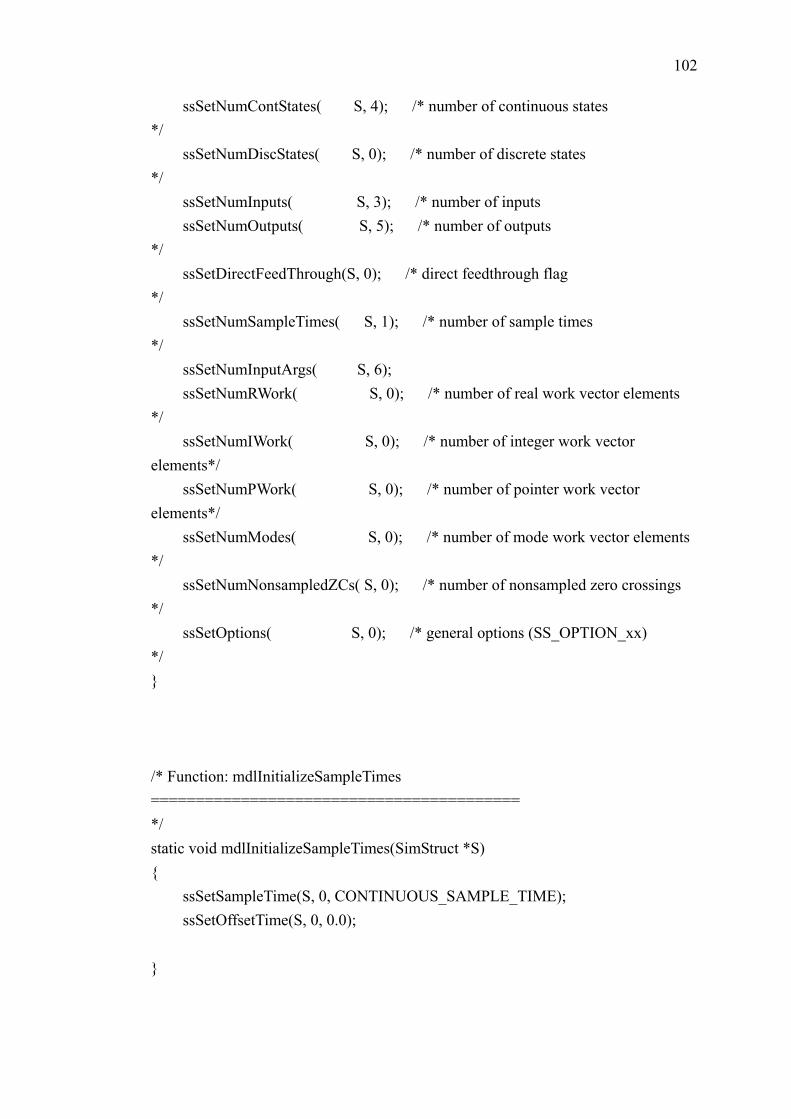
102
ssSetNumContStates( S, 4); /* number of continuous states */ ssSetNumDiscStates( S, 0); /* number of discrete states */ ssSetNumInputs( S, 3); /* number of inputs ssSetNumOutputs( S, 5); /* number of outputs */ ssSetDirectFeedThrough(S, 0); /* direct feedthrough flag */ ssSetNumSampleTimes( S, 1); /* number of sample times */ ssSetNumInputArgs( S, 6); ssSetNumRWork( S, 0); /* number of real work vector elements */ ssSetNumIWork( S, 0); /* number of integer work vector elements*/ ssSetNumPWork( S, 0); /* number of pointer work vector elements*/ ssSetNumModes( S, 0); /* number of mode work vector elements */ ssSetNumNonsampledZCs( S, 0); /* number of nonsampled zero crossings */ ssSetOptions( S, 0); /* general options (SS_OPTION_xx) */ } /* Function: mdlInitializeSampleTimes ========================================= */ static void mdlInitializeSampleTimes(SimStruct *S) { ssSetSampleTime(S, 0, CONTINUOUS_SAMPLE_TIME); ssSetOffsetTime(S, 0, 0.0); }
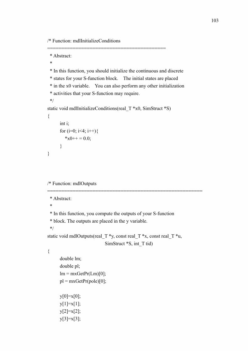
103
/* Function: mdlInitializeConditions ========================================== * Abstract: * * In this function, you should initialize the continuous and discrete * states for your S-function block. The initial states are placed * in the x0 variable. You can also perform any other initialization * activities that your S-function may require. */ static void mdlInitializeConditions(real_T *x0, SimStruct *S) { int i; for (i=0; i<4; i++){ *x0++ = 0.0; } } /* Function: mdlOutputs ======================================================= * Abstract: * * In this function, you compute the outputs of your S-function * block. The outputs are placed in the y variable. */ static void mdlOutputs(real_T *y, const real_T *x, const real_T *u, SimStruct *S, int_T tid) { double lm; double pl; lm = mxGetPr(Lm)[0]; pl = mxGetPr(pole)[0]; y[0]=x[0]; y[1]=x[1]; y[2]=x[2]; y[3]=x[3];
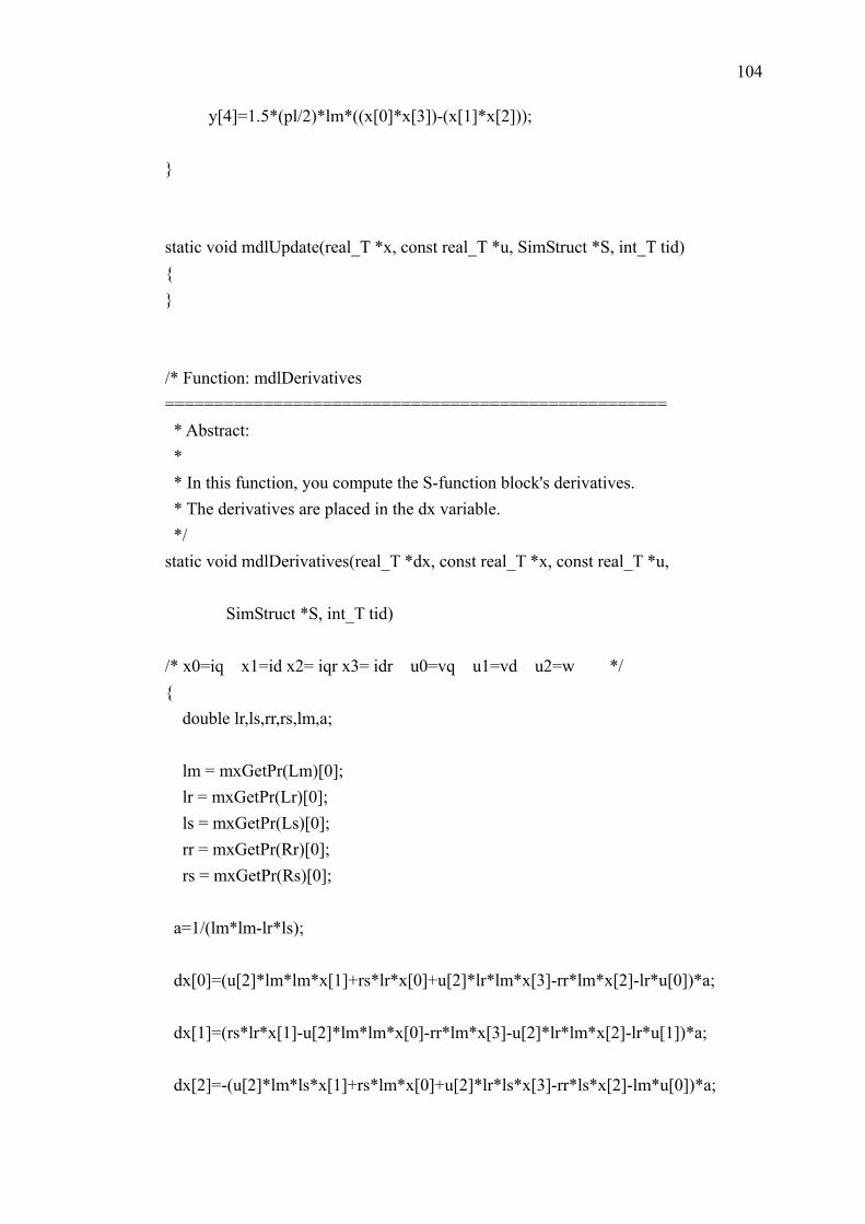
104
y[4]=1.5*(pl/2)*lm*((x[0]*x[3])-(x[1]*x[2])); } static void mdlUpdate(real_T *x, const real_T *u, SimStruct *S, int_T tid) { } /* Function: mdlDerivatives =================================================== * Abstract: * * In this function, you compute the S-function block's derivatives. * The derivatives are placed in the dx variable. */ static void mdlDerivatives(real_T *dx, const real_T *x, const real_T *u, SimStruct *S, int_T tid) /* x0=iq x1=id x2= iqr x3= idr u0=vq u1=vd u2=w */ { double lr,ls,rr,rs,lm,a; lm = mxGetPr(Lm)[0]; lr = mxGetPr(Lr)[0]; ls = mxGetPr(Ls)[0]; rr = mxGetPr(Rr)[0]; rs = mxGetPr(Rs)[0]; a=1/(lm*lm-lr*ls); dx[0]=(u[2]*lm*lm*x[1]+rs*lr*x[0]+u[2]*lr*lm*x[3]-rr*lm*x[2]-lr*u[0])*a; dx[1]=(rs*lr*x[1]-u[2]*lm*lm*x[0]-rr*lm*x[3]-u[2]*lr*lm*x[2]-lr*u[1])*a; dx[2]=-(u[2]*lm*ls*x[1]+rs*lm*x[0]+u[2]*lr*ls*x[3]-rr*ls*x[2]-lm*u[0])*a;
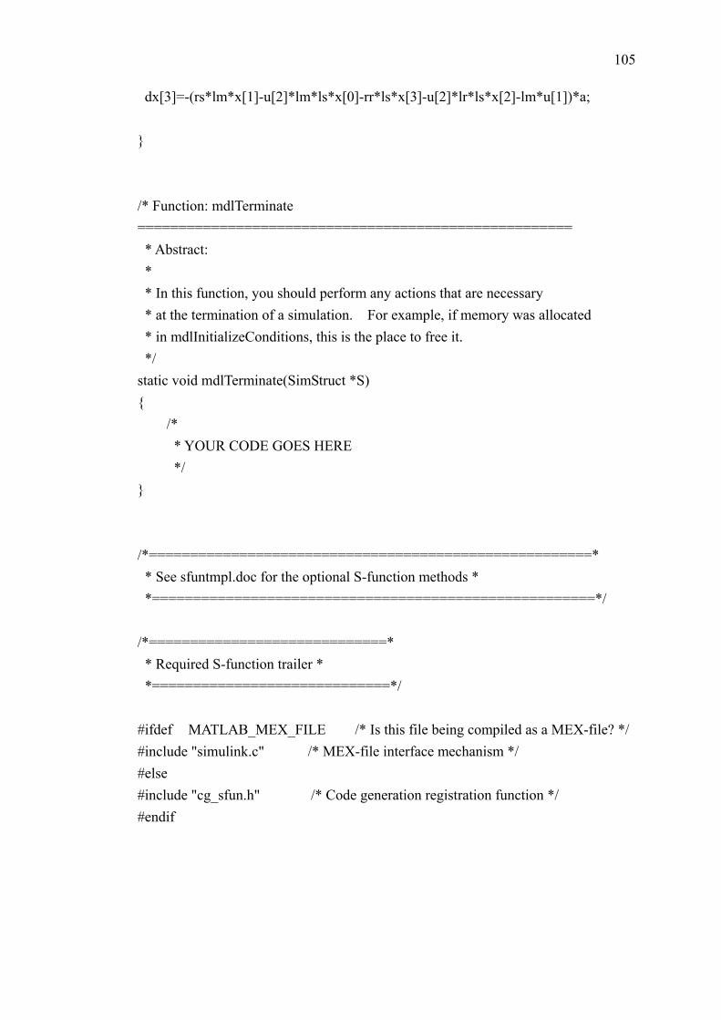
105
dx[3]=-(rs*lm*x[1]-u[2]*lm*ls*x[0]-rr*ls*x[3]-u[2]*lr*ls*x[2]-lm*u[1])*a; } /* Function: mdlTerminate ===================================================== * Abstract: * * In this function, you should perform any actions that are necessary * at the termination of a simulation. For example, if memory was allocated * in mdlInitializeConditions, this is the place to free it. */ static void mdlTerminate(SimStruct *S) { /* * YOUR CODE GOES HERE */ } /*======================================================* * See sfuntmpl.doc for the optional S-function methods * *======================================================*/ /*=============================* * Required S-function trailer * *=============================*/ #ifdef MATLAB_MEX_FILE /* Is this file being compiled as a MEX-file? */ #include "simulink.c" /* MEX-file interface mechanism */ #else #include "cg_sfun.h" /* Code generation registration function */ #endif
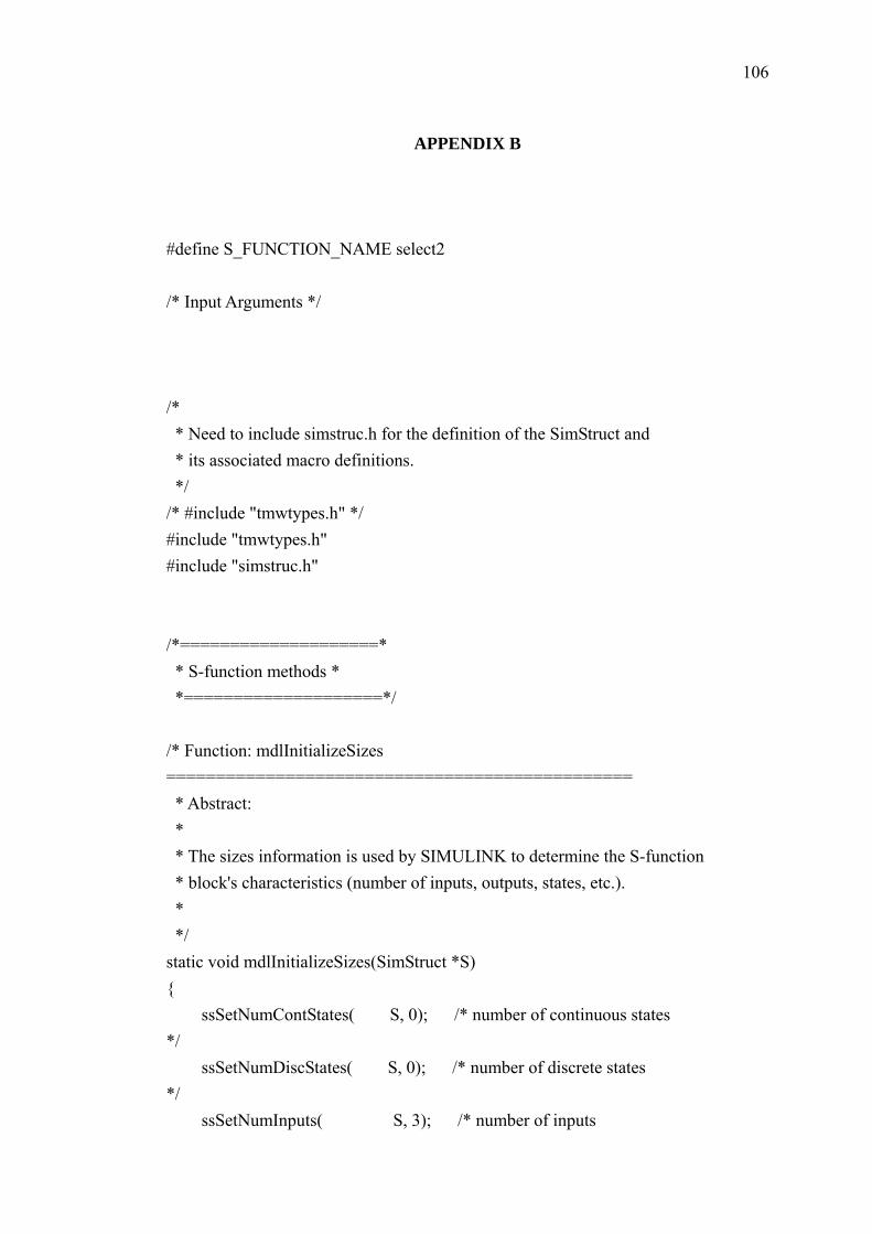
106
APPENDIX B
#define S_FUNCTION_NAME select2 /* Input Arguments */ /* * Need to include simstruc.h for the definition of the SimStruct and * its associated macro definitions. */ /* #include "tmwtypes.h" */ #include "tmwtypes.h" #include "simstruc.h" /*====================* * S-function methods * *====================*/ /* Function: mdlInitializeSizes =============================================== * Abstract: * * The sizes information is used by SIMULINK to determine the S-function * block's characteristics (number of inputs, outputs, states, etc.). * */ static void mdlInitializeSizes(SimStruct *S) { ssSetNumContStates( S, 0); /* number of continuous states */ ssSetNumDiscStates( S, 0); /* number of discrete states */ ssSetNumInputs( S, 3); /* number of inputs
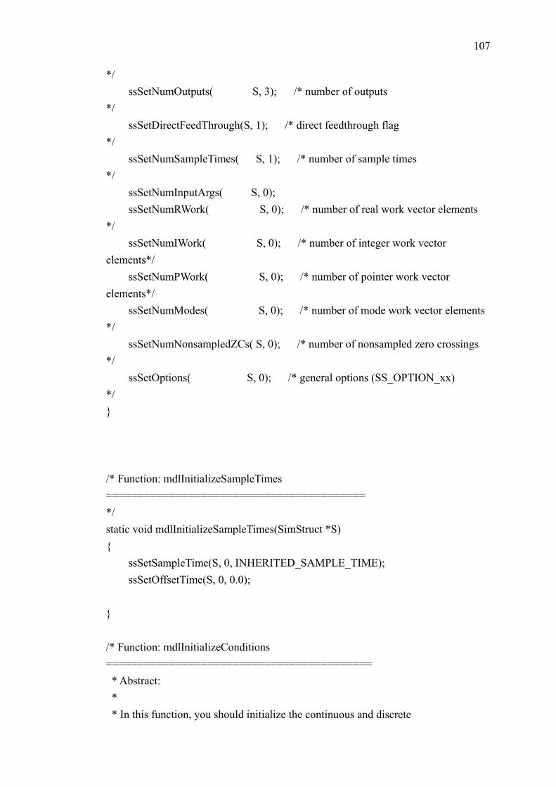
107
*/ ssSetNumOutputs( S, 3); /* number of outputs */ ssSetDirectFeedThrough(S, 1); /* direct feedthrough flag */ ssSetNumSampleTimes( S, 1); /* number of sample times */ ssSetNumInputArgs( S, 0); ssSetNumRWork( S, 0); /* number of real work vector elements */ ssSetNumIWork( S, 0); /* number of integer work vector elements*/ ssSetNumPWork( S, 0); /* number of pointer work vector elements*/ ssSetNumModes( S, 0); /* number of mode work vector elements */ ssSetNumNonsampledZCs( S, 0); /* number of nonsampled zero crossings */ ssSetOptions( S, 0); /* general options (SS_OPTION_xx) */ } /* Function: mdlInitializeSampleTimes ========================================= */ static void mdlInitializeSampleTimes(SimStruct *S) { ssSetSampleTime(S, 0, INHERITED_SAMPLE_TIME); ssSetOffsetTime(S, 0, 0.0); } /* Function: mdlInitializeConditions ========================================== * Abstract: * * In this function, you should initialize the continuous and discrete
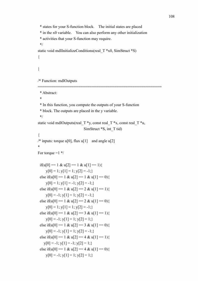
108
* states for your S-function block. The initial states are placed * in the x0 variable. You can also perform any other initialization * activities that your S-function may require. */ static void mdlInitializeConditions(real_T *x0, SimStruct *S) { } /* Function: mdlOutputs ======================================================= * Abstract: * * In this function, you compute the outputs of your S-function * block. The outputs are placed in the y variable. */ static void mdlOutputs(real_T *y, const real_T *x, const real_T *u, SimStruct *S, int_T tid) { /* inputs: torque u[0], flux u[1] and angle u[2] * For torque =1 */ if(u[0] == 1 & u[2] == 1 & u[1] == 1){ y[0] = 1; y[1] = 1; y[2] = -1;} else if(u[0] == 1 & u[2] == 1 & u[1] == 0){ y[0] = 1; y[1] = -1; y[2] = -1;} else if(u[0] == 1 & u[2] == 2 & u[1] == 1){ y[0] = -1; y[1] = 1; y[2] = -1;} else if(u[0] == 1 & u[2] == 2 & u[1] == 0){ y[0] = 1; y[1] = 1; y[2] = -1;} else if(u[0] == 1 & u[2] == 3 & u[1] == 1){ y[0] = -1; y[1] = 1; y[2] = 1;} else if(u[0] == 1 & u[2] == 3 & u[1] == 0){ y[0] = -1; y[1] = 1; y[2] = -1;} else if(u[0] == 1 & u[2] == 4 & u[1] == 1){ y[0] = -1; y[1] = -1; y[2] = 1;} else if(u[0] == 1 & u[2] == 4 & u[1] == 0){ y[0] = -1; y[1] = 1; y[2] = 1;}
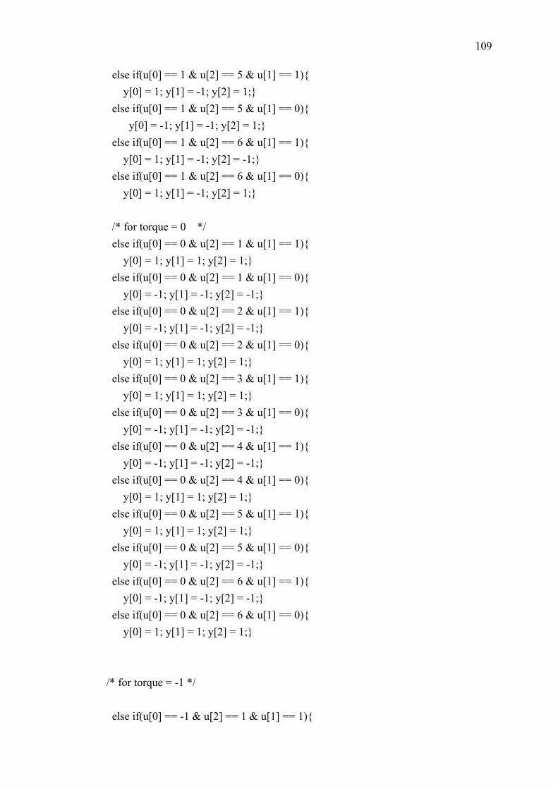
109
else if(u[0] == 1 & u[2] == 5 & u[1] == 1){ y[0] = 1; y[1] = -1; y[2] = 1;} else if(u[0] == 1 & u[2] == 5 & u[1] == 0){ y[0] = -1; y[1] = -1; y[2] = 1;} else if(u[0] == 1 & u[2] == 6 & u[1] == 1){ y[0] = 1; y[1] = -1; y[2] = -1;} else if(u[0] == 1 & u[2] == 6 & u[1] == 0){ y[0] = 1; y[1] = -1; y[2] = 1;} /* for torque = 0 */ else if(u[0] == 0 & u[2] == 1 & u[1] == 1){ y[0] = 1; y[1] = 1; y[2] = 1;} else if(u[0] == 0 & u[2] == 1 & u[1] == 0){ y[0] = -1; y[1] = -1; y[2] = -1;} else if(u[0] == 0 & u[2] == 2 & u[1] == 1){ y[0] = -1; y[1] = -1; y[2] = -1;} else if(u[0] == 0 & u[2] == 2 & u[1] == 0){ y[0] = 1; y[1] = 1; y[2] = 1;} else if(u[0] == 0 & u[2] == 3 & u[1] == 1){ y[0] = 1; y[1] = 1; y[2] = 1;} else if(u[0] == 0 & u[2] == 3 & u[1] == 0){ y[0] = -1; y[1] = -1; y[2] = -1;} else if(u[0] == 0 & u[2] == 4 & u[1] == 1){ y[0] = -1; y[1] = -1; y[2] = -1;} else if(u[0] == 0 & u[2] == 4 & u[1] == 0){ y[0] = 1; y[1] = 1; y[2] = 1;} else if(u[0] == 0 & u[2] == 5 & u[1] == 1){ y[0] = 1; y[1] = 1; y[2] = 1;} else if(u[0] == 0 & u[2] == 5 & u[1] == 0){ y[0] = -1; y[1] = -1; y[2] = -1;} else if(u[0] == 0 & u[2] == 6 & u[1] == 1){ y[0] = -1; y[1] = -1; y[2] = -1;} else if(u[0] == 0 & u[2] == 6 & u[1] == 0){ y[0] = 1; y[1] = 1; y[2] = 1;} /* for torque = -1 */ else if(u[0] == -1 & u[2] == 1 & u[1] == 1){
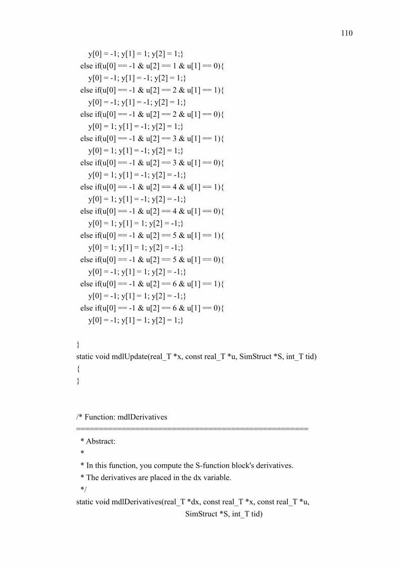
110
y[0] = -1; y[1] = 1; y[2] = 1;} else if(u[0] == -1 & u[2] == 1 & u[1] == 0){ y[0] = -1; y[1] = -1; y[2] = 1;} else if(u[0] == -1 & u[2] == 2 & u[1] == 1){ y[0] = -1; y[1] = -1; y[2] = 1;} else if(u[0] == -1 & u[2] == 2 & u[1] == 0){ y[0] = 1; y[1] = -1; y[2] = 1;} else if(u[0] == -1 & u[2] == 3 & u[1] == 1){ y[0] = 1; y[1] = -1; y[2] = 1;} else if(u[0] == -1 & u[2] == 3 & u[1] == 0){ y[0] = 1; y[1] = -1; y[2] = -1;} else if(u[0] == -1 & u[2] == 4 & u[1] == 1){ y[0] = 1; y[1] = -1; y[2] = -1;} else if(u[0] == -1 & u[2] == 4 & u[1] == 0){ y[0] = 1; y[1] = 1; y[2] = -1;} else if(u[0] == -1 & u[2] == 5 & u[1] == 1){ y[0] = 1; y[1] = 1; y[2] = -1;} else if(u[0] == -1 & u[2] == 5 & u[1] == 0){ y[0] = -1; y[1] = 1; y[2] = -1;} else if(u[0] == -1 & u[2] == 6 & u[1] == 1){ y[0] = -1; y[1] = 1; y[2] = -1;} else if(u[0] == -1 & u[2] == 6 & u[1] == 0){ y[0] = -1; y[1] = 1; y[2] = 1;} } static void mdlUpdate(real_T *x, const real_T *u, SimStruct *S, int_T tid) { } /* Function: mdlDerivatives =================================================== * Abstract: * * In this function, you compute the S-function block's derivatives. * The derivatives are placed in the dx variable. */ static void mdlDerivatives(real_T *dx, const real_T *x, const real_T *u, SimStruct *S, int_T tid)
111
{ } /* Function: mdlTerminate ===================================================== * Abstract: * * In this function, you should perform any actions that are necessary * at the termination of a simulation. For example, if memory was allocated * in mdlInitializeConditions, this is the place to free it. */ static void mdlTerminate(SimStruct *S) { } /*======================================================* * See sfuntmpl.doc for the optional S-function methods * *======================================================*/ /*=============================* * Required S-function trailer * *=============================*/ #ifdef MATLAB_MEX_FILE /* Is this file being compiled as a MEX-file? */ #include "simulink.c" /* MEX-file interface mechanism */ #else #include "cg_sfun.h" /* Code generation registration function */ #endif


