Pertanika 3(2), 162-165 (1980)

SHORT COMMUNICATION (III)

Income and Price Elasticities of Demand for Domestic Water:A Case Study of Alor Setar, Kedah.

RINGKASAN

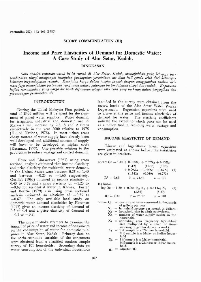
Satu analisa rentasan untuk isi-isi rumah di Alar Setal', Kedah, menunjukkan yang keluarga ber­pendapatan tinggi mempunyai keanjalar: pendapatan perm~ntaan air lima kali ganda lebih dari keluarga­keluarga berpendapatan rendah. KeanJalan harga dalam Jangka pendek dengan menggunakan analisa siri­masa juga menunjukkan perbezaan yang sama antara gulungan berpendapatan tinggi dan rendah. Keputusankajian menunjukkan yang harga air boleh digunakan sebagai satu cara yang berkesan dalam pengagihan danperancangan pembekalan air.

INTRODUCTION

During the Third Malaysia Plan period, atotal of $496 million will be spent for develop­ment of piped water supplies. Water demandfor irrigation, industrial and domestic use inMalaysia will increase by 2.3, 8 and 2 timesrespectively in the year 2000 relative to 1975(United Nations, 1976). In most urban areascheap sources of water supply have already beenwell developed and additional sources of supplywill have to be developed at higher costs(Katzman, 1977). One possible solution to theproblem is to reduce wastage and control demand.

Howe and Linaweaver (1967) using crosssectional analysis estimated that income elasticityand price elasticity for residential water demandin the United States were between 0.35 to 1.40and between -0.23 to -1.60 respectively.Gottlieb (1963) obtained an income elasticity of0.45 to 0.58 and a price elasticity of -1.23 to-0.68 for residential water in Kansas. Fosterand Beattie (1979) also using cross sectionalanalysis estimated an elasticity of -0.35 to-0.67. The only available local study ondomestic water demand elasticities by Katzman(1977) gives an income elasticity of demand of0.2 to 0.4 and a price elasticity of demand of-0.1 to -0.2.

The present study attempts to examine theimpact of price of water and income of consumerson the consumption of water for domestic pur­poses in Alor Setar, Kedah. Primary data onthe socio-economic variables of the consumerswere obtained from a stratified random samplesurvey of 101 households. Secondary data onwater consumption of the individual households

162

included in the survey were obtained from therecord books of the Alor Setar Water WorksDepartment. Regression equations were usedto arrive at the price and income elasticities ofdemand for water. The elasticity coefficientsindicate the extent to which price can be usedas a policy tool in reducing water wastage andconsumption.

INCOME ELASTICITY OF DEMAND

Linear and logarithmic linear equationswere estimated as shown below; the t-statisticsare given in brackets.

linear: Qc = 1.10 + 0.018Xl + 7.67X2 + 6.1 5X3

(4.12) (10.36) (3.49)+ 0.09)4 + 0.49Xs + 0.62X6 (1)

(1.342) (0.089) (0.273)R2 = 0.63 F = 24.43 n = 101

log linear:log Qc = 1.20 + 0.301 log Xl + 0.54 log X2 (2)

(3.86) (5.20)R2 = 0.37 F = 25.17 n = 101

where Qc = quantity of water consumed in thousandsof gallons per year.

Xl household income per month in dOllars.X2 household size in adult equivalents.X3 number of water supply outlets in the

household.X4 sprinkling area frequency (sprinkling

area multiplied by number of timeswatering of garden done in a week).

Xs 1 if sample is a Chinese household.o if sample is a Malay or Indian house­hold.

X6 1 if sample is a Malay household.oif sample is a Chinese or Indian house­hold.

R2 adjusted R2

MOHD. ARIFF HUSSEIN AND K. KUPERAN

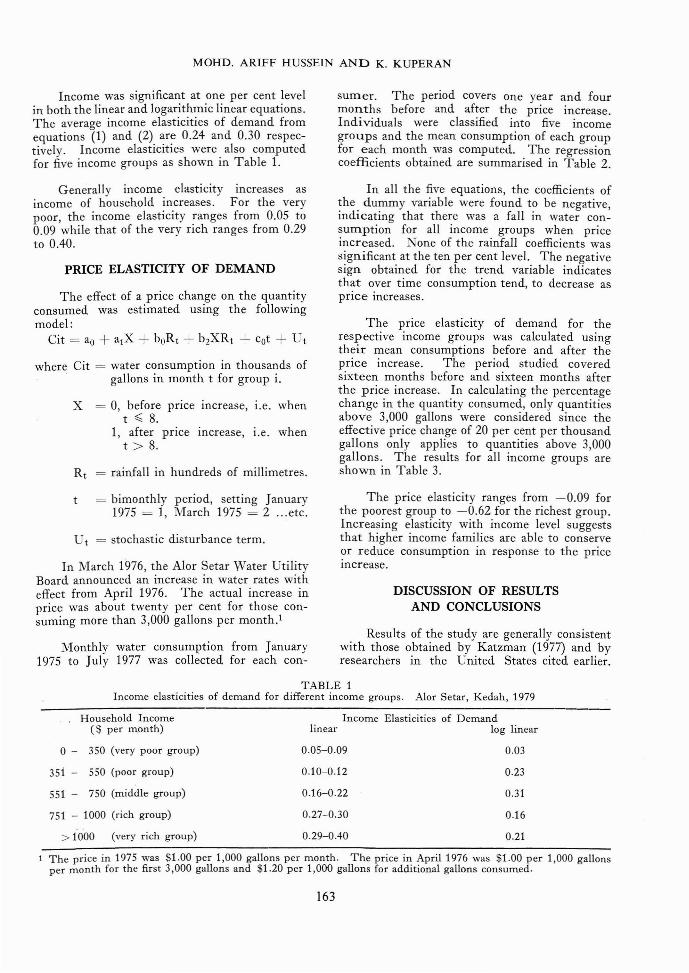
Income was significant at one per cent levelin both the linear and logarithmic linear equations.The average income elasticities of demand fromequations (1) and (2). ~r~ 0.24 and 0.30 respec­tively. Income elasticities were also computedfor five income groups as shown in Table 1.

Generally income elasticity increases asincome of household increases. For the verypoor, the income elasticity ranges from 0.05 to0.09 while that of the very rich ranges from 0.29to 0.40.

PRICE ELASTICITY OF DEMAND

The effect of a price change on the quantityconsumed was estimated using the followingmodel:

Cit = ao + atX + boRt + b 2XRt + cot + U t

where Cit = water consumption in thousands of. gallons in month t for group i.

x = 0, before price increase, i.e. whent ::;; 8.

1, after price increase, i.e. whent> 8.

Rt = rainfall in hundreds of millimetres.

t = bimonthly period, setting January1975 = 1, March 1975 = 2 ... etc.

U t = stochastic disturbance term.

In March 1976, the Alor Setar Water UtilityBoard announced an increase in water rates witheffect from April 1976. The actual increase inprice was about twenty per cent for those con­suming more than 3,000 gallons per month.1

Monthly water consumption from January1975 to July 1977 was collected for each con-

sumer. The period covers one year and fourmonths before and after the price increase.Individuals were classified into five incomegroups and the mean consumption of each groupfor each month was computed. The regressioncoefficients obtained are summarised in Table 2.

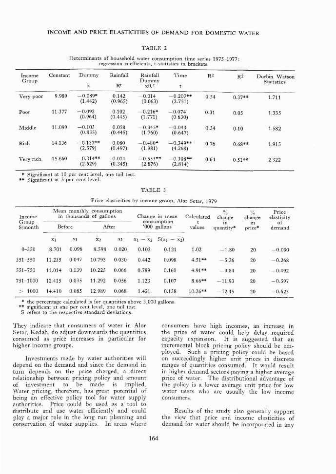
In all the five equations, the coefficients ofthe dummy variable were found to be negative,indicating that there was a fall in water con­sumption for all income groups when priceincreased. None of the rainfall coefficients wassignificant at the ten per cent level. The negativesign obtained for the trend variable indicatesthat over time consumption tend, to decrease asprice increases.

The price elasticity of demand for therespective income groups was calculated usingtheir mean consumptions before and after theprice increase. The period studied coveredsixteen months before and sixteen months afterthe price increase. In calculating the percentagechange in the quantity consumed, only quantitiesabove 3,000 gallons were considered since theeffective price change of 20 per cent per thousandgallons only applies to quantities above 3,000gallons. The results for all income groups areshown in Table 3.

The price elasticity ranges from -0.09 forthe poorest group to -0.62 for the richest group.Increasing elasticity with income level suggeststhat higher income families are able to conserveor reduce consumption in response to the priceincrease.

DISCUSSION OF RESULTSAND CONCLUSIONS

Results of the study are generally consistentwith those obtained by Katzman (1977) and byresearchers in the United States cited earlier.

TABLE 1Income elasticities of demand for different income groups. Alor Setar, Kedah, 1979

Income Elasticities of Demandlinear log linear

Household Income($ per month)

o - 350 (very poor group)

3si - 550 (poor group)

551 - 750 (middle group)

751 - 1000 (rich group)

> 1000 (very rich group)

0.05-0.09

0.10-0.12

0.16-0.22

0.27-0.30

0.29-0.40

0.03

0.23

0.31

0.16

0.21

1 The price in 1975 was $1.00 per 1,000 gallons per month. The price in April 1976 was $1.00 per 1,000 gallonsper month for the first 3,000 gallons and $1.20 per 1,000 gallons for additional gallons consumed.

163

INCOME AND PRICE ELASTICITIES OF DEMAND FOR DOMESTIC WATER

TABLE 2

Determinants of household water consumption time series 1975-1977:regression coefficients, t-statistics in brackets

Income Constant Dummy Rainfall Rainfall Time R2 R2 Durbin WatsonGroup Dummy Statistics

x Rt xR t t

Very poor 9.989 -0.089" 0.142 -0.014 -0.207.... 0.54 0.37.... 1.711(1.442) (0.965) (0.063) (2.751)

Poor 11.377 -0.092 0.102 -0.216" -0.074 0.31 0.05 1.335(0.964) (0.445) (1.771) (0.630)

Middle 11.099 -0.103 0.058 -0.345" -0.043 0.34 0.10 1.582(0.835) (0.445) (1.760) (0.647)

Rich 14.136 -0.137.... 0.080 -0.480" -0.349.... 0.76 0.68.... 1.915(2.579) (0.497) (1.981) (4.268)

Very rich 15.660 -0.314.... 0.074 -0.533.... -0.308.... 0.64 0.51 .... 2.322(2.629) (0.345) (2.876) (2.814)

.. Significant at 10 per cent level, one tail test ..... Significant at 5 per cent level.

TABLE 3

Price elasticities by income group, Alor Setar, 1979

Mean monthly consumption % % PriceIncome in thousands of gallons Change in mean Calculated change change elasticityGroup consumption t m m ofS/month Before After '000 gallons values quantity" price" demand

Xl sl X2 S2 XI - x2 S(iZl - X2)

0-350 8.701 0.096 8.598 0.020 0.103 0.121 1.02 -1.80 20 -0.090

351-550 11.235 0.047 10.793 0.030 0.442 0.098 4.51 .... -5.36 20 -0.268

551-750 11.014 0.139 10.225 0.066 0.789 0.160 4.91 .... -9.84 20 -0.492

751-1000 12.415 0.035 11.292 0.056 1.123 0.107 8.66.... -11.93 20 -0.597

> 1000 14.410 0.085 12.989 0.068 1.421 0.138 10.26.... -12.45 20 -0.623

.. the percentage calculated is for quantities above 3,000 gallons..... significant at one per cent level, one tail test.S refers to the respective standard deviations.

They indicate that consumers of water in AlorSetar, Kedah, do adjust downwards the quantitiesconsumed as price increases in particular forhigher income groups.

Investments made by water authorities willdepend on the demand and since the demand inturn depends on the price charged, a directrelationship between pricing policy and amountof investment to be made is implied.\iVater pricing, therefore, h2.s gre2.t potential ofbeing an effective policy tool for water supplyauthorities. Price could be used as a tool todistribute and use water efficiently and couldplaya major role in the long run planning andconservation of water supplies. In areas where

164

consumers have high incomes, an increase inthe price of water could help delay requiredcapacity expansion. It is suggested that anincremental block pricing policy should be em­ployed. Such a pricing policy could be basedon succeedingly higher unit prices in discreteranges of quantities consumed. It would resultin higher demand sectors paying a higher averageprice of water. The distributional advantage ofthe policy is a lower average unit price for lowwater users who are usually the low incomeconsumers.

Results of the study also generally supportthe view that price and income elasticities ofdemand for water should be incorporated in any

MOHD. ARIFF HUSSEIN AND K. KUPERAN

projection of water demand. Future studiesshould concentrate on the relevant ranges ofprice changes that wil1 make significant differencesin the design systems and storage capacities ofa water utility.

Mohd. Ariff Hussein andK. Kuperan

Faculty of Resource Economics and AgribusinessUniversiti Pertanian Malaysia,Serdang, Selangor.

REFERENCES

FOSTER, H.S. JR. and BEATTIE, B.R. (1979): UrbanResidential Demand for Water in the UnitedStates. Land Eco1lS. 55, 43-58.

GOTTLIEB, M. (1963): Urban Domestic Demand forWater: Arkansas Case Study. Land Econs. 39,204-210.

GOVERNMENT OF MALAYSIA (1970): The Third Malay­sia Plan, Prime Minister's Department Malaysia.

HOWE, C.W. and LINAWEAVER, J.P. (1967): TheImpact of Pr ce on Residential Water Demandand Its Relation to System Design and PriceStructure. Water Resources Research. Vol. 3.First Quarter, 1967, 13-32.

KATZMAN, MARTIN, T.K. (1977): Income and PriceElasticities of Demand for Water in DevelopingCountries. Water Resources Bulletin Vol. XLLLNo. I, February 1977, 47-55.

A ON. (1976): Secr~tariate, Malaysian National Com­mittee of the International Hydrological Pro­gramme, c/o Drainage and Irrigation DivisionKuala Lumpur (1976); United rations Water

Conference Country Report for Malaysia. Paperpresented at ESCAP Regional preparatory meeting:Bangkok. July 27 - August 2, 1976.

(Received 18 June 1980)

•

165