from optimal control problems to foliations, some kinds of multifoliations … · 2011-03-07 ·...

FROM OPTIMAL CONTROL PROBLEMS TO FOLIATIONS, SOME KINDS OFMULTIFOLIATIONS AND RELATIONS TO GENERALISED JETS

(Daripada Masalah Kawalan Optimum kepada Foliasi, Beberapa Jenis Multifoliasidan Hubungan dengan Jet Teritlak)

MIROSLAV KURES

ABSTRACT

Transversal foliations and jets modulo foliations are studied. It is shown that multifoliations providesa way for a more general description of (R, S, Q)-jets.Keywords: Optimal control; regulation; foliation; multifoliation; transversality; jet; (R, S, Q)-jet

ABSTRAK

Foliasi rentas lintang dan jet modulo foliasi dikaji. Ditunjukkan bahawa multifoliasi membuka jalanuntuk pemerihalan yang lebih umum bagi jet-(R, S, Q).Kata kunci: Kawalan optimum; regulasi; foliasi; multifoliasi; kerentas-lintangan; jet; jet-(R, S, Q)

1. Introduction

This paper represents an extended version of the author’s contribution (Kures 2008) to the Inter-national Symposium on New Developments of Geometric Function Theory and its Applications,Bangi 2008. In particular, the first section is completely new and it represents a possible motivationfor a study of foliations and multifoliations. It refers to fundamentals of geometric optimal controltheory and it also refers to some classical examples (cf. Chapter 15 of La Valle (2006)) which areelaborated in detail here. The second section is focused to the study of foliations of smooth mani-folds. We introduce concepts of ∩-transversality and ∪-transversality as we hope that this approachprovides a more precise view to the transversality in itself and gives a good arrangement of variousmultifoliated structures. Further, we initialise jet formalism for such multifoliated structures. Wehave two main inspirations here: Ikegami’s paper (Ikegami 1986) about jets modulo foliations andthe concept of (R, S, Q)-jet, see e.g. Kolar et al. (1993) or Doupovec & Kolar (1999). We presenta way to a generalisation and unification (in a way) of both these jet languages.

We remark that multifoliations can be meaningfully used just in the optimal control. Indeed,partitions of manifolds induced by integrable distributions even satisfy some of transversality con-ditions (introduced in Section 2) in a number of practical situations.

As usually, all manifolds and maps are assumed to be smooth, i.e. of class C∞.

Journal of Quality Measurement and Analysis JQMA 6(2) 2010, 19-32Jurnal Pengukuran Kualiti dan AnalisisJournal of Quality Measurement and Analysis JQMA 6(2) 2010, 19-32Jurnal Pengukuran Kualiti dan AnalisisJournal of Quality Measurement and Analysis JQMA 6(2) 2010, 19-32Jurnal Pengukuran Kualiti dan Analisis

Journal of Quality Measurement and Analysis JQMA 6(2) 2010, 19-32Jurnal Pengukuran Kualiti dan Analisis

2. Possible motivations for study of foliations by differential geometry

2.1. Lie bracket

Let M be a smooth manifold, dimM = m, for an initial simplification it suffices think aboutM = Rm. Points of M are written as

x = (x1, . . . , xm), x0 = (x10, . . . , x

m0 ), etc. (1)

We consider a smooth map γ : I → M , where I is an interval in R, usually containing 0. Such amap is called a (smooth) curve in M . Its equations1 are

xi = γi(t), i = 1, . . . , m. (2)

Let γ(0) = x0, then dγdt (0) determines a tangent vector to γ in x0 with coordinates

(x1

0, . . . , xm0 , y1

0, . . . , ym0

)=

(γ1(0), . . . , γm(0),

dγ1

dt(0), . . . ,

dγm

dt(0)

). (3)

Tangent vectors to all curves γ going through x0 form a m-dimensional vector space Tx0M , tangentspace in x0. The vector coordinates are

(x1

0, . . . , xm0 , y1, . . . , ym

). (4)

We define the tangent bundle TM by the (disjoint) union

TM =⋃

x0∈M

Tx0M ; (5)

TM is 2m-dimensional as a manifold with coordinates(x1, . . . , xm, y1, . . . , ym

)= (x, y). (6)

We have a canonical projection π : TM → M sending (x, y) to (x). The vector field on M is asmooth section X : M → TM , i.e. such a smooth map, for which π ◦X = idM . In coordinates,

X :(x1, . . . , xm

) 7→ (x1, . . . , xm, ξ1(x), . . . , ξm(x)

)(7)

and X(x0) is (for a fixed point x0) a tangent vector as in (3). If f : M → R is a smooth functionand X a vector field on M , we define a new function Xf : M → R called the Lie derivative of falong X by

Xf(x0) =∂f

∂xiξi(x0). (8)

We also write Xf = ∂f∂xi ξ

i and X = ξi ∂∂xi . The vector field X is called smooth, if Xf is smooth

for every smooth function f . If X is a given vector field on M , then the integral curve ofX is sucha curve γ which has a tangent vector in every its pointx0 equal to X(x0), i.e.

(dγ1

dt, . . .

dγm

dt

)=

(ξ1(γ(t)), . . . , ξm(γ(t))

); (9)

1for a general M ( 6= Rm) we have local expressions in local coordinates

20

Miroslav KurešMiroslav KurešMiroslav Kureš

for a finding of integral curves is necessary to solve a system of m first order ordinary differentialequations

γ = X(γ). (10)

In particular, we apply maximal integral curves: such a integral curve can not be a proper subset ofanother integral curve. If γx : I → M is a maximal integral curve of X satisfying γx(0) = x, then,by

FlXt (x) = FlX(t, x) = γx(t), (11)

are defined maps

FlXt : M → M and FlX : I ×M → M. (12)

The map FlX is called the flow 2 of the vector field X . Evidently,

ddt

FlXt (x) = X(FlXt (x)

)(13)

holds. The important property of the flow is

FlX(t + s, x) = FlX(t, FlX(s, x)

). (14)

A real vector space V is called the Lie algebra, if it contains a binary operation named the bracketand denoting by [, ] having the following properties:

1. (u, v) 7→ [u, v] is bilinear,

2. (u, v) 7→ [u, v] is antisymmetric,

3. Jacobi identity [u, [v, w]] + [v, [w, u]] + [w, [u, v]] = 0 holds.

We define the Lie bracket [X, Y ] of vector fields X = ξi ∂∂xi , Y = ηi ∂

∂i by

[X, Y ]f = X(Yf)− Y (Xf), (15)

it follows coordinates of Z = [X, Y ] = ζi ∂∂xi are

ζi = ξj ∂ηi

∂xj− ηj ∂ξi

∂xj(16)

and this bracket provides the structure of Lie algebra to every vector space Tx0M . We say thatvector fields X, Y commute, if [X, Y ] = 0.

2the flow maps the point x to another point lying just on the maximal curve going through x; viewing this curve as amotion, x has time 0 and its image a time t

2121

From optimal control problems to foliations, some kinds of multifoliations and relations to generalised jets

2.2. Why is the Lie bracket so important in optimal control

The system (10) can be written as

xi = ξi(x) = ξi(x1, . . . , xm), i = 1, . . . , m. (17)

In optimal control, we investigate the system

xi = φi(x, u) = φi(x1, . . . , xm, u1, . . . , uk), i = 1, . . . , m, (18)

where u1(t), . . . , uk(t) is so-called regulation3. The linear system has a form

xi = Aijx

j + Bipu

p, i = 1, . . . , m, (19)

otherwise we have nonlinear systems. A frequent nonlinear system is so-called affine system

x = Xp(x)up + X0(x), p = 1, . . . , k (20)

where X1, . . . , Xk, X0 are vector fields. For X0 = 0, we talk about the driftless affine system (X0

is called the drift term). In particular, let us consider a driftless affine optimal control system

x = X(x)u1 + Y (x)u2, where u(t) =(u1(t), u2(t)

)=

(1, 0) for t ∈ [0, ε](0, 1) for t ∈ [ε, 2ε](−1, 0) for t ∈ [2ε, 3ε](0,−1) for t ∈ [3ε, 4ε]

(21)

We compute Taylor expansions for the first part of the motion as

x(ε) = x(0) + εx(0) +12ε2x(0) +O(ε3)

= x(0) + εX(x(0)) +12ε2

∂X

∂x(x(0))X(x(0)) +O(ε3), (22)

and for the second part as

x(2ε) = x(ε) + εx(ε) +12ε2x(ε) +O(ε3)

= x(ε) + εY (x(ε)) +12ε2

∂Y

∂x(x(ε))Y (x(ε)) +O(ε3), (23)

in which we substitute x(ε) from (22) and use the fact that for the infinitesimal ε the relationY (x(0) + X(x(0))) = ε∂Y

∂x (x(0))X(x(0)) holds 4; we obtain

x(2ε) = x(0) + Y (x(0)

+ ε2(

12

∂X

∂x(x(0))X(x(0)) +

∂Y

∂x(x(0))X(x(0)) +

12

∂Y

∂x(x(0))Y (x(0))

)(24)

+ O(ε3).3see the next section4this fact is a slight generalisation of the well-known expression f(x0 + ε) ≈ εf ′(x0) for a function f and a point x0

22


The same process is used for x(3ε) and x(4ε), the final result is

x(4ε) = x(0) + ε2(

∂Y

∂x(x(0))X(x(0))− ∂X

∂x(x(0))Y (x(0))

)+ O(ε3). (25)

The computation shows that, at each point, infinitesimal motion is possible not only in the directionscontained in the span of the input vector fields X and Y , but also in the directions of their Lie bracket[X, Y ] = ∂Y

∂x X− ∂X∂x Y . It is also possible to obtain motion in the direction of higher-order brackets,

such as [X, [X, Y ]], [Y, [X, Y ]], etc.

2.3. A note about regulations

For the regulation u : R → Rk, u(t) =(u1(t), . . . , uk(t)

)are not any requirements for a smooth-

ness nor even for a continuity of functions up : R → R, p = 1, . . . , k. Hereafter regulations areconsidered to be piecewise constant functions, it means there is a partition of the time line intointervals and in every such an interval J is

u(t) = c = (c1, . . . , ck), t ∈ J, cp, p = 1, . . . , k, are real constants. (26)

(Cf. (21) as an example.) Moreover, only some special subclasses of piece-wise constant functionsare considered. Then we talk about admissible regulations and the subclass of admissible regulationsis denoted by U, so we write u ∈ U.

2.4. Distributions and foliations

Suppose that for each x0 ∈ M and k < m a k-dimensional vector subspace Dx0M of Tx0M . Letus consider the (disjoint) union

DM =⋃

x0∈M

Dx0M. (27)

The k-distribution on M is a smooth section D : M → DM , i.e. such a map, which assigns to eachpoint x0 such a k-dimensional subspace. This is possible by such a way that

D(x) = span{X1(x), . . . , Xk(x)}, (28)

where X1, . . . , Xk are linear independent smooth vector fields. Nevertheless, if arbitrary vectorfields X1, . . . , Xk are given, then a dimension of span{X1(x), . . . , Xk(x)} can be less than k andcan differ in different points. (Such a map is counted as a distribution, not a k-distribution.) LetD be a k-distribution on M and N a n-dimensional submanifold of M , n ≤ k. Then N is said anintegral manifold of D, if Tx0N ⊆ D(x0). An integral manifold of D is called the maximal integralmanifold if it is not contained in any strictly larger integral manifold of D. The k-distribution D onM is called an integrable distribution, if each point of M is contained in some integral manifoldof D. Then each point is contained in a unique maximal integral manifold, so the maximal integralmanifolds form a partition of M . This partition is called the foliation of M induced by the integrabledistribution D, and each maximal integral manifold is called a leaf of this foliation. Further, we saythat a vector field X lies in D, if X(x0) ∈ D(x0) for all x0 ∈ M . If X lies in D, then integral

2323


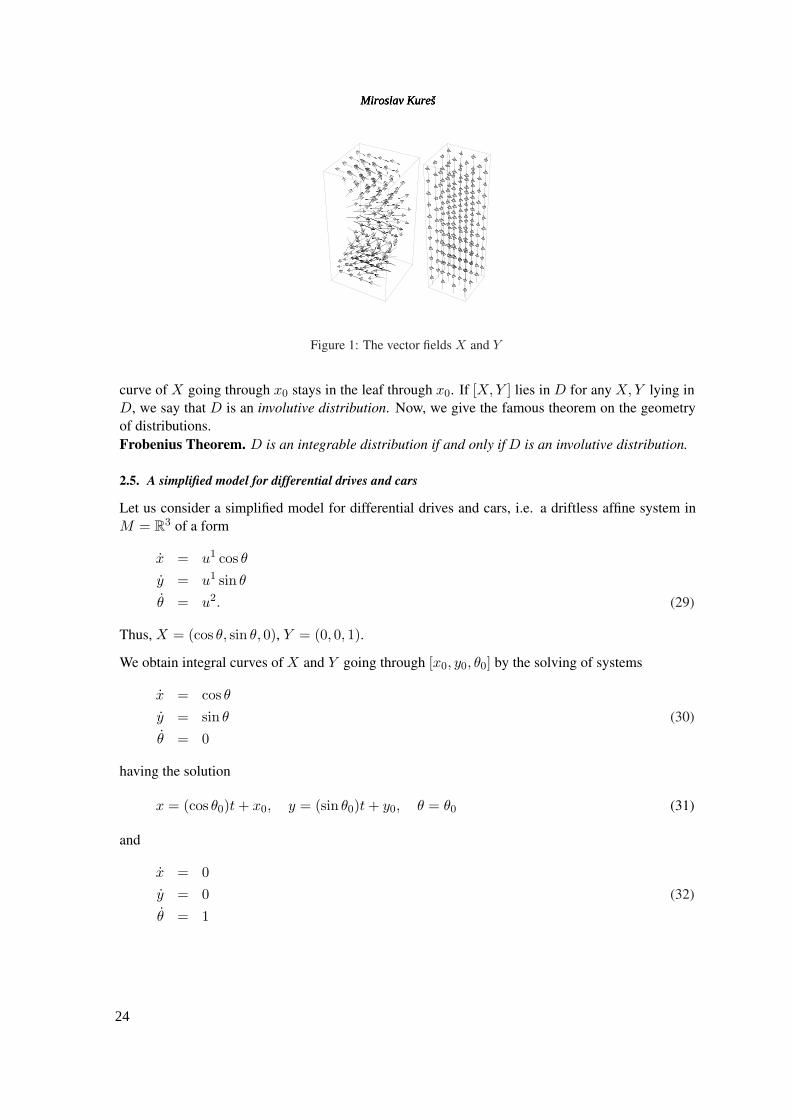
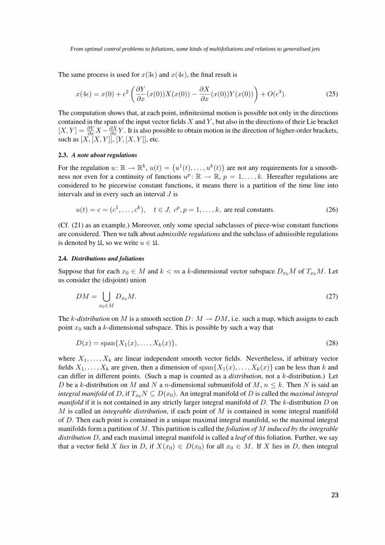
Figure 1: The vector fields X and Y

curve of X going through x0 stays in the leaf through x0. If [X, Y ] lies in D for any X, Y lying inD, we say that D is an involutive distribution. Now, we give the famous theorem on the geometryof distributions.Frobenius Theorem. D is an integrable distribution if and only if D is an involutive distribution.

2.5. A simplified model for differential drives and cars

Let us consider a simplified model for differential drives and cars, i.e. a driftless affine system inM = R3 of a form

x = u1 cos θ

y = u1 sin θ

θ = u2. (29)

Thus, X = (cos θ, sin θ, 0), Y = (0, 0, 1).

We obtain integral curves of X and Y going through [x0, y0, θ0] by the solving of systems

x = cos θ

y = sin θ (30)

θ = 0

having the solution

x = (cos θ0)t + x0, y = (sin θ0)t + y0, θ = θ0 (31)

and

x = 0y = 0 (32)

θ = 1

24


-1.0

-0.5

0.0

0.5

1.0

-1.0

-0.5

0.0

0.5

1.0

0.0

0.5

1.0

1.5

2.0

-1.0

-0.5

0.0

0.5

1.0

-1.0

-0.5

0.0

0.5

1.0

0.0

0.5

1.0

1.5

2.0

Figure 2: The integral curves of X and Y

having the solution

x = x0, y = y0, θ = t + θ0. (33)

The distribution D maps every point to a plane given by this point and by direction vectors of linesabove:

D : (x0, y0, θ0) 7→ {(x0, y0, θ0) + u1(cos θ0, sin θ0, 0) + u2(0, 0, 1);u1, u2 ∈ R} (34)

The distribution is a 2-distribution, because it is 2-dimensional in every point. Nevertheless,

[X, Y ] = (sin θ,− cos θ, 0) (35)

and this vector field is not a linear combination of X and Y . Hence [X, Y ] does not lie in D and Dis not involutive. By Frobenius theorem, D is not integrable.

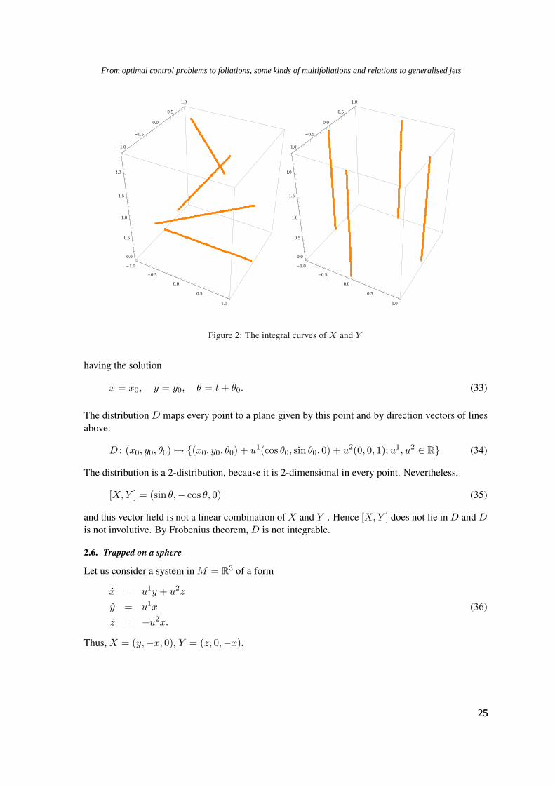
2.6. Trapped on a sphere

Let us consider a system in M = R3 of a form

x = u1y + u2z

y = u1x (36)

z = −u2x.

Thus, X = (y,−x, 0), Y = (z, 0,−x).

2525


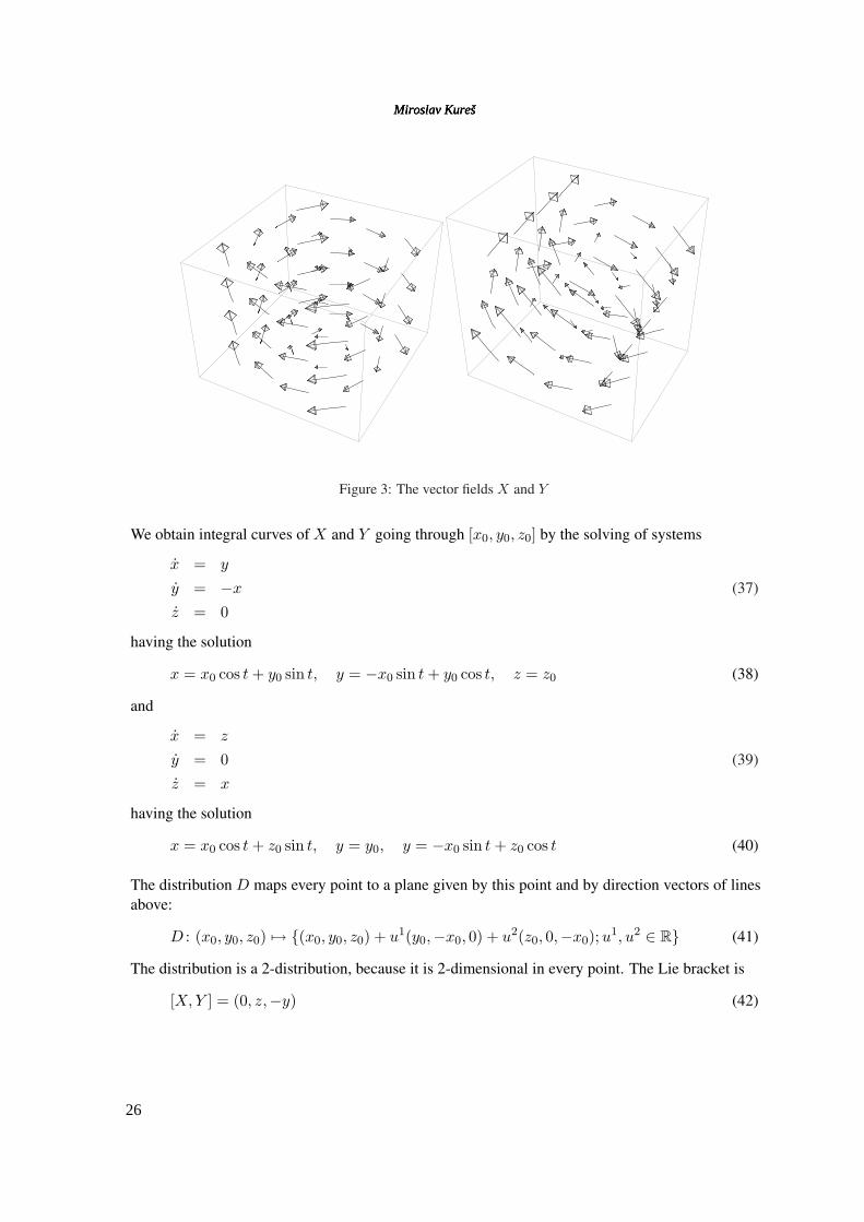
Figure 3: The vector fields X and Y

We obtain integral curves of X and Y going through [x0, y0, z0] by the solving of systems

x = y

y = −x (37)

z = 0

having the solution

x = x0 cos t + y0 sin t, y = −x0 sin t + y0 cos t, z = z0 (38)

and

x = z

y = 0 (39)

z = x

having the solution

x = x0 cos t + z0 sin t, y = y0, y = −x0 sin t + z0 cos t (40)

The distribution D maps every point to a plane given by this point and by direction vectors of linesabove:

D : (x0, y0, z0) 7→ {(x0, y0, z0) + u1(y0,−x0, 0) + u2(z0, 0,−x0);u1, u2 ∈ R} (41)

The distribution is a 2-distribution, because it is 2-dimensional in every point. The Lie bracket is

[X, Y ] = (0, z,−y) (42)

26


-2

0

2

-2

0

2

-1.0

-0.5

0.0

0.5

1.0

-2

0

2

-1.0-0.5

0.00.5

1.0

-2

0

2

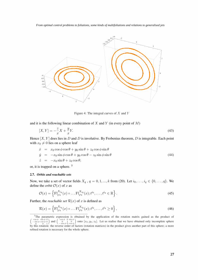
Figure 4: The integral curves of X and Y

and it is the following linear combination of X and Y (in every point of M )

[X, Y ] = − z

xX +

y

xY. (43)

Hence [X, Y ] does lies in D and D is involutive. By Frobenius theorem, D is integrable. Each pointwith x0 6= 0 lies on a sphere leaf

x = x0 cosφ cos θ + y0 sin θ + z0 cosφ sin θ

y = −x0 sinφ cos θ + y0 cos θ − z0 sinφ sin θ (44)

z = −x0 sin θ + z0 cos θ;

or, it is trapped on a sphere. 5

2.7. Orbits and reachable sets

Now, we take a set of vector fields Xq , q = 0, 1, ..., k from (20). Let i0, . . . , iq ∈ {0, . . . , q}. Wedefine the orbit O(x) of x as

O(x) ={

FlXiq

tiq(x) ◦ . . .Fl

Xi0

ti0(x); ti0 , . . . , tiq ∈ R

}. (45)

Further, the reachable set R(x) of x is defined as

R(x) ={

FlXiq

tiq(x) ◦ . . .Fl

Xi0

ti0(x); ti0 , . . . , tiq ≥ 0

}, (46)

5The parametric expression is obtained by the application of the rotation matrix gained as the product of(cos φ sin φ 0− sin φ cos φ 0

0 0 1

)and

(cos φ 0 sin φ

0 1 0− sin φ 0 cos φ

)onto [x0, y0, z0]. Let us realise that we have obtained only incomplete sphere

by this rotation: the reverse order of factors (rotation matrices) in the product gives another part of this sphere; a morerefined rotation is necessary for the whole sphere.

2727


the reachable set R(x, τ) in time τ of x is defined as

R(x, τ) ={

FlXiq

tiq(x) ◦ . . .Fl

Xi0

ti0(x); ti0 , . . . , tiq ≥ 0, ti0 + · · ·+ tiq = τ

}(47)

and the reachable set RT (x) until time T of x is defined as

RT (x) =⋃

τ≤T

R(x, τ) ={

FlXiq

tiq(x) ◦ . . .Fl

Xi0

ti0(x); ti0 , . . . , tiq ≥ 0, ti0 + · · ·+ tiq ≤ T

}(48)

There are two notable restrictions of sets above. The first one is a restriction on admissible regula-tions and the second one is a restriction on trajectories contained in a given neighborhood V of x.Then we write, e.g., RU

T (x), RVT (x), RU,V

T (x).

3. The foliations again and more precisely, and moreover the multifoliations

3.1. Foliations

We refer to Milnor (1970), Lawson (1974) and Bejancu and Farran (2006) for detailed introductionsto the theory of foliations; our adoption is as follows. Let M be a m-dimensional smooth manifold,m = p + q, m ∈ N, p, q ∈ N ∪ {0}, (x, y) = (x1, . . . , xp, y1, . . . , yq) ∈ Rp × Rq = Rm. Forconstants c ∈ Rp, c ∈ Rq, we consider spaces Rq

c = {(x, y) ∈ Rm;x1 = c1, . . . , xp = cp} andRp

c = {(x, y) ∈ Rm; y1 = c1, . . . , yq = cq}. Intersections of Rqc and Rp

c with open sets (balls)with respect to the standard topology are denoted by P q

c and P pc and called the (c, q)-coplaque and

the (p, c)-plaque in Rm. Suppose that F = {Lt}t∈J is a partition of M into connected subsets,M =

⋃t∈J Lt, Lt ∩ Ls = ∅ for t 6= s. Further, we consider a foliated atlas on M , i.e., a collection

{Ui, ϕi}i∈I , ϕi = αi × βi, αi : Ui → Rp, βi : Ui → Rq, of charts satisfying

(i) {Ui}i∈I is a cover of M by open sets

(ii) each connected component of Lt ∩ Ui (for all i ∈ I , t ∈ J) is mapped by ϕi onto an (p, c)-plaque in Rm, i.e., for u ∈ Ui

xa = αai (u) a = 1, . . . , p (49)

yb = βbi (u) = cb b = 1, . . . , q

(iii) transition functions ϕij = ϕj ◦ ϕ−1i on Ui ∩ Uj , ϕij = αij × βij , send (p, c)-plaques onto

(p, c)-plaques, i.e.

xa = αaij(x, y) a = 1, . . . , p (50)

yb = βbij(y) b = 1, . . . , q.

(Maps are regarded as smooth.) ThenF is called the foliation of M of dimension p and codimensionq, Lt, t ∈ J leaves of F and M the foliated manifold written shortly by (M,F). Trivial cases arisefor p = 0, q = m (leaves = points) and for p = m, q = 0 (the unique leaf = M ).

Let F , F ′ be two foliations of M with dimensions p and p′. Then F ′ is called a subfoliation ofF and F is called a superfoliation of F ′, denoted by F ′ ¹ F , if the following conditions hold:

28


(i) 0 ≤ p′ ≤ p ≤ m

(ii) for any leaf L′ of F ′, there exists a leaf L of F such that L′ ⊆ L, and the restriction of F ′ ona leaf L of F is a foliation of dimension p− p′ of L.

The relation ¹ is an order in the set of foliations of M .Fibered manifolds are canonically foliated, their fibers can be viewed as leaves. On the other

hand, there exist manifolds, which are foliated but not fibered.

3.2. Transversality of maps, transversality of foliations, multifoliations

Concepts of a transversality is rather varied, we suggest e.g. Tamura & Sato (1981). Let ∆ be aninteger greater than 1. Let us consider manifolds Hδ, δ = 1, . . . ,∆, and M . Let fδ : Hδ → M ,δ = 1, . . . ,∆, be (smooth) maps.

We take an arbitrary non-empty subset E ⊆ {1, . . . ,∆} and denote by Im fE the intersection ofall images of fε, ε ∈ E.

For uE ∈ Im fE and every ε ∈ E, let (Tfε)uE denote the image of the tangent map to fε inuE ; tangent vectors belonging to (Tfε)uE generate a vector subspace of TuEM ; we denote it by〈(Tfε)uE 〉. Further, we denote by 〈⋃

E

(Tfε)uE 〉 the vector space generated by the union of vectors

in all (Tfε)uE , ε ∈ E, and by 〈⋂E

(Tfε)uE 〉 the vector space generated by vectors belonging to the

intersection of all (Tfε)uE , ε ∈ E.For simplicity, we consider only maps for which vector spaces above have constant dimensions

for all uE ∈ Im fE .Now, it is evident that for every chosen ε0 ∈ E

0 ≤ dim〈⋂

E

(Tfε)uE 〉 ≤ dim〈(Tfε0)uE 〉 ≤ dim〈⋃

E

(Tfε)uE 〉 ≤ m, (51)

or, in the codimension language,

m ≥ codim〈⋂

E

(Tfε)uE 〉 ≥ codim〈(Tfε0)uE 〉 ≥ codim〈⋃

E

(Tfε)uE 〉 ≥ 0. (52)

Definition 1 Maps fδ : Hδ → M , δ = 1, . . . ,∆, are said to be

∩-transversal, if

codim〈⋂

E

(Tfε)uE 〉 =∑

E

codim〈(Tfε)uE 〉 (53)

for all E ⊆ {1, . . . ,∆};

∪-transversal, if∑

E

dim〈(Tfε)uE 〉 = dim〈⋃

E

(Tfε)uE 〉 (54)

for all E ⊆ {1, . . . ,∆}.

2929


Remark 1 The Definition 1 implies that fδ can be ∩-transversal only for

∆∑

δ=1

codim〈(Tfδ)u{1,...,∆}〉 ≤ m (55)

and, analogously, fδ can be ∪-transversal only for

∆∑

δ=1

dim〈(Tfδ)u{1,...,∆}〉 ≤ m. (56)

It is easy to show that

∆∑

δ=1

codim〈(Tfδ)u{1,...,∆}〉 ≤ m and∆∑

δ=1

dim〈(Tfδ)u{1,...,∆}〉 ≤ m (57)

comes into being simultaneously only for ∆ = 2 and codim〈(Tf1)u{1,2}〉+ codim〈(Tf2)u{1,2}〉 =dim〈(Tf1)u{1,2}〉 + dim〈(Tf2)u{1,2}〉 = m. In this special case, concepts of ∩-transversality and∪-transversality are identical.

Let us consider ∩-transversal maps fδ : Hδ → M , δ = 1, . . . ,∆ in the following situation: Hδ

are subsets (submanifolds) of M and fδ : Hδ → M are their inclusion maps (immersions). ThenHδ are called ∩-transversal, too. Moreover, if we have ∆ foliations Fδ of M , we take in everyu ∈ M their leaves: if they are ∩-transversal on each choice of u, we say that foliations Fδ of Mare ∩-transversal.

The concept ∪-transversal foliations Fδ of M comes quite analogously.

Definition 2 A collection F = {Fδ}∆δ=1 of foliations of M (dimM = m) with dimensions pδ and

codimensions qδ is called the ∩-multifoliation (∪-multifoliation), if foliations Fk are ∩-transversal(∪-transversal). Especially, the ∩-multifoliation (∪-multifoliation) is called total ∩-multifoliation(total ∪-multifoliation) if ∆ = m.

Remark 2 It is clear that q1 = · · · = q∆ = 1 for total ∩-multifoliation and p1 = · · · = p∆ = 1 fortotal ∪-multifoliation.

3.3. Jets modulo multifoliations

G. Ikegami has defined in his paper (Ikegami 1986) jets modulo foliations. We generalise his con-cept by the following definition. (In this section, we mean by a multifoliation either∩-multifoliationor ∪-multifoliation.)

Definition 3 Let H , M be two manifolds, f, g : H → M maps satisfying f(h) = g(h) = u ∈ Mand let F = {Fδ}∆

δ=1 be a multifoliation of M . Then f is said to have the (r1, . . . , r∆)-multiordercontact modulo F with g at u, if for every ∆-tuple of charts

{U δ 3 u, ϕδ

}1≤δ≤∆

the maps

αδ ◦ f : U δ → Rpδ and αδ ◦ g : U δ → Rpδ (58)

30


belong to the same (classical) rδ-jet at u. (It means that for every curve γ : R→ H with γ(0) = h,the curves αδ ◦ f ◦ γ and αδ ◦ g ◦ γ have the rδ-order contact in zero.) As the relation ”have the(r1, . . . , r∆)-multiorder contact modulo F” is evidently an equivalence relation, we denote the classof maps having the (r1, . . . , r∆)-multiorder contact modulo F with f at u by

jr1,...,r∆

h f mod F (59)

and call it (r1, . . . , r∆)-jet modulo the multifoliation F with the source h ∈ H and the targetu = f(h) ∈ M .

We denote by Jr1,...,r∆

h (H, M ;F)u the set of all (r1, . . . , r∆)-jets modulo the multifoliation Fwith the h and the target u. Further, we denote

Jr1,...,r∆

h (H, M ;F) =⋃

u∈M

Jr1,...,r∆

h (H, M ;F)u, (60)

Jr1,...,r∆(H, M ;F)u =⋃

h∈H

Jr1,...,r∆

h (H, M ;F)u (61)

and

Jr1,...,r∆(H, M ;F) =⋃

u∈M

⋃

h∈H

Jr1,...,r∆

h (H, M ;F)u. (62)

For manifolds H and M and a multifoliation F of M , Jr1,...,r∆

h (H, M ;F)u, Jr1,...,r∆

h (H, M ;F),Jr1,...,r∆(H, M ;F)u, and Jr1,...,r∆(H, M ;F) have a smooth manifold structure. We have bundleprojections

Jr1,...,r∆(H, M ;F) → H and Jr1,...,r∆(H, M ;F) → M (63)

as well as canonical bundle projections

Jr1,...,r∆(H, M ;F) → J r1,...,r∆(H, M ;F) (64)

by restricting the multiorder, i.e. for 0 ≤ r1 ≤ r1, . . . , 0 ≤ r∆ ≤ r∆. In doing so

J0,...,0(H, M ;F) = H ×M. (65)

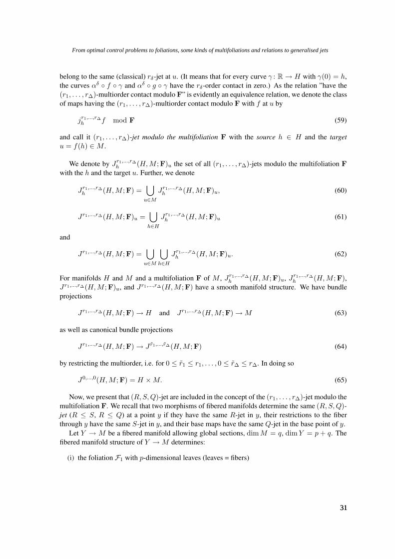
Now, we present that (R, S, Q)-jet are included in the concept of the (r1, . . . , r∆)-jet modulo themultifoliation F. We recall that two morphisms of fibered manifolds determine the same (R, S, Q)-jet (R ≤ S, R ≤ Q) at a point y if they have the same R-jet in y, their restrictions to the fiberthrough y have the same S-jet in y, and their base maps have the same Q-jet in the base point of y.

Let Y → M be a fibered manifold allowing global sections, dimM = q, dimY = p + q. Thefibered manifold structure of Y → M determines:

(i) the foliation F1 with p-dimensional leaves (leaves = fibers)

3131


(ii) the foliation F2 with q-dimensional leaves (leaves = suitable smooth sections, e.g. for vectorbundles can be taken smooth sections including zero section, such as constant smooth sectionsor something like that); F2 is non-unique

Thus, we have a (non-unique) multifoliation which is simultaneously∪-multifoliation and∩-multifoliation,see Remark 1. Our construction implies:

Theorem 1 Let F be a multifoliation given by the fibration as stated above. Then there is a repre-sentation of every (R, S, Q)-jet as a (S, Q)-jet modulo F.

Acknowledgements

The author would like to thank the organisers of the International Symposium on New Developmentsof Geometric Function Theory and its Applications, Bangi, Malaysia, 2008, for the great organisa-tion, hospitality and interest. The authors’ participation in the conference was supported by theMinistry of Education, Youth and Sports of the Czech Republic, research plan MSM 0021630518.This paper was written using the subsidisation of the GACR, grant No. 201/09/0981.

References

Bejancu A. & Farran H. R. 2006. Foliations and Geometric Stuctures. Berlin: Springer Verlag.Doupovec M. & Kolar I. 1999. On the jets of fibred manifold morphisms. Cah. Topologie Geom. Differ. Categ. 40: 21–30.Ikegami G. 1986. Vector fields tangent to foliations. Japan J. Math. 12: 95–120.Kolar I., Michor P.W. & Slovak J. 1993. Natural Operations in Differential Geometry. Berlin: Springer Verlag.Kures M. 2008. Foliations and multifoliations: a note on transversalities and generalisations of jets, in: Proc. Inter. Symp.

on New Devel. of Geom. Funct. Theory and its Appl., Bangi 2008, Editors: M. Darus & S. Owa, 2008, 390–394.La Valle S.M. 2006. Planning Algorithms. Cambridge: Cambridge University Press.Lawson Jr. H. B. 1974. Foliations. Bull. Amer. Math. Soc. 80: 369–418.Milnor J. 1970. Foliations and Foliated Vector Bundles, mimeographed lecture notes from a course given at MIT, 62 pp.Tamura I. & Sato A. 1981. On transverse foliations. Publ. Math. Inst. Etud. Sci. 54: 205–235.

Institute of MathematicsBrno University of TechnologyTechnicka 261669 BrnoCzech RepublicE-mail: [email protected]

32


from optimal control problems to foliations, some kinds of multifoliations … · 2011-03-07 ·...

Documents