PertanikaJ. Sci. & Technol. 3(1) :37-43( 1995)ISSN: 0128-7680

© niversiti Pertanian Malaysia Press

Estimation of Parameters in aNon-linear Model

Salleh HarunPhysics Department

Faculty of Science and Environmental StudiesUniversiti Pertanian Nlalaysia

43400 UPM, Serdang, Selangor DaTUl Ehsan, Malaysia

Received 22 January 1993

ABSTRAK

Pelbagai proses kimia dan biologi boleh dirangkapkan dalam bentuk fungsi taklinear yang mengandungi beberapa eksponen. Satu kaedah yang cekap tetapikurang digunakan untuk menentukan parameter-parameter di dalam fungsitersebut ialah dengan memadankan data kepada suatu model. Kertas kerja inimenghuraikan penggunaan subrutin NAG, E04HFF dan LSFUN2 bagi analisisdata yang disimulasi dan mengandungi dua eksponen. Data itu juga mengandungiselisih bebas bertabur normal. Bagi sisihan dengan selisih piawai kurang daripada0.3, kaedah ini menyakinkan dan cekap. Pekali-pekali linear dan pemalar masayang pendek boleh ditentukan dengan kejituan melebihi 98%. Apabila sisihanpiawai melebihi 2.0, selisih-selisih di dalam parameter boleh melebihi 12%.

ABSTRACT

A wide variety of chemical and biophysical processes are describable in a non­linear function consisting of a number of exponentials. An efficient but seldom­used method to estimate the parameters is by fitting the data to a model. Thispaper describes the use of NAG subroutines E04HFF and LSFUN2 for the non­linear analysis of simulated data which conform to a model consisting of twoexponentials. The data have been generated with independent and normallydistributed errors. For errors with standard deviation less than 0.3, the methodproves to be reliable and efficient. The linear coefficient and the shorter timeconstant have been obtained with an accuracy better than 98%. However, whenthe standard deviation of the error is greater than 2.0, the error in the estimat­ed parameters can be as large as 12%.

Keywords: NMR non-linear, data fitting

INTRODUCTION

Some experimen ts in physical and biophysical sciences yield data which canbe expressed as a sum of exponentials. Fitting the data to a model enablesthe identification of the system or the determination of the parameters ofthe model. In a biological system, one may use a mathematical model todescribe the concentrations and amount of a substance as a function of time.In medicine and physiology, compartmental analysis is often used to study

Salleh Harun

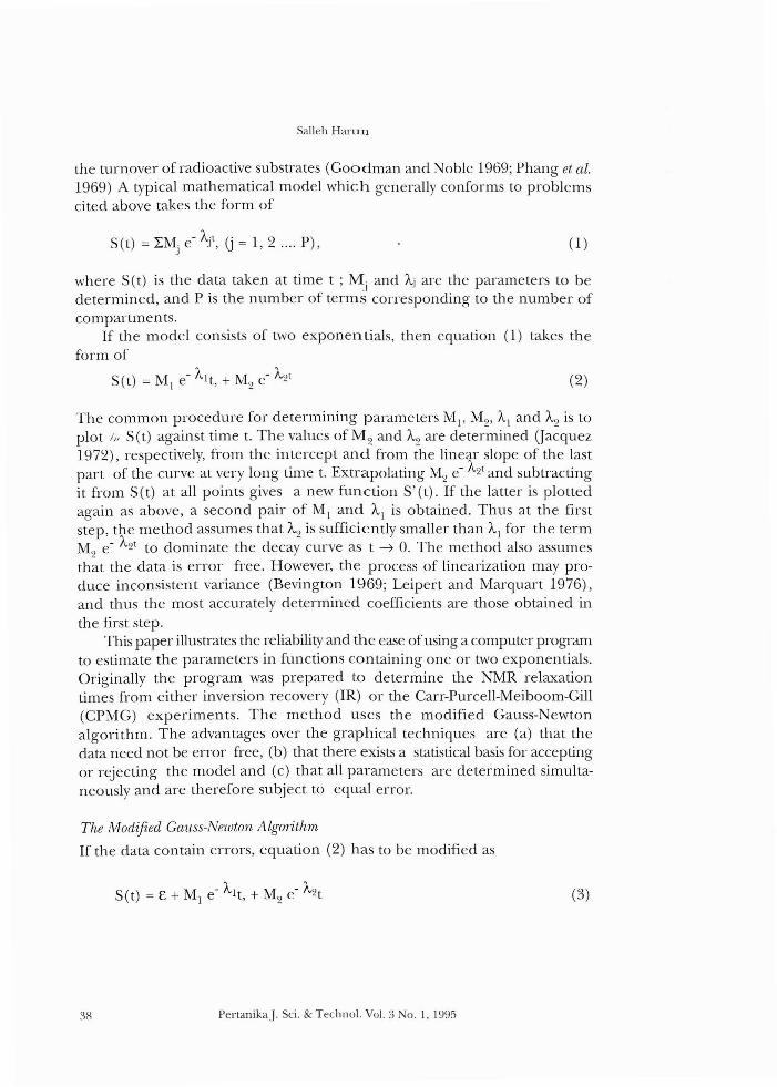
the turnover ofradioactive substrates (Goodman and Noble 1969; Phang et al.1969) A typical mathematical model which generally conforms to problemscited above takes the form of

S(t) = LM e- Al, (j = 1,2 .... P),J

(1)

where S(t) is the data taken at time t ; M j and Aj are the parameters to bedetermined, and P is the number of terms corresponding to the number ofcompartmen ts.

If the model consists of two exponen tials, then equation (l) takes theform of

S(t) = M1

e- Al t, + M2

e- A2 t (2)

The common procedure for determining parameters Ml' M2, A, and A2 is toplot I" S(t) against time t. The values ofM2 and A2 are determined (Jacquez1972), respectively, from the intercept and from the linear slope of the lastpart of the curve at very long time t. Extrapolating M2 e- A2

t and subtractingit from S( t) at all points gives a new function S' (t). If the latter is plottedagain as above, a second pair of M, and A,] is obtained. Thus at the firststep, the method assumes that A2 is sufficiently smaller than AI for the termM~ e- A,21 to dominate the decay curve as t ~ O. The method also assumesth;t the data is error free. However, the process of linearization may pro­duce inconsistent variance (Bevington 1969; Leipert and Marquart 1976),and thus the most accurately determined coefficients are those obtained inthe first step.

This paper illustrates the reliability and the ease of using a computer programto estimate the parameters in functions containing one or two exponentials.Originally the program was prepared to determine the NMR relaxationtimes from either inversion recovery (IR) or the Carr-Purcell-Meiboom-Gill(CPMG) experiments. The method uses the modified Gauss-Newtonalgorithm. The advantages over the graphical techniques are (a) that thedata need not be error free, (b) that there exists a statistical basis for acceptingor rejecting the model and (c) that all parameters are determined simulta­neously and are therefore subject to equal error.

The Modified Gauss-Newton Algorithm

If the data contain errors, equation (2) has to be modified as

38 PertanikaJ. Sci. & Technol. Vol. 3 0.1,1995

(3)

Estimation of Parameters in a Non·linear Model

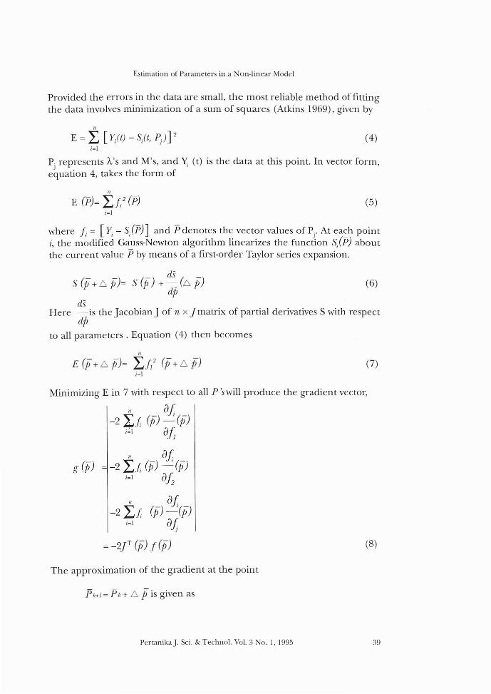
Provided the errors in the data are small, the most reliable method of fittingthe data involves minimization of a sum of squares (Atkins 1969), given by

II

E = L. [y,(t) - S/t, Ij)Pi=l

(4)

Pjrepresents A's and M's, and Y; (t) is the data at this point. In vector form,

equation 4, takes the form of

II

E (1')= L.J/ (1')i=1

(5)

where !J = [Yi - slJ5)] and l' denotes the vector values of Pj . At ea~h poin ti, the modified Gauss-Newton algorithm linearizes the function S/P) aboutthe current value l' by means of a first-order Taylor series expansion.

dsS (fi + 6 fi)= S (fi) + -. (6 fi) (6)

dpds

Here -.is the Jacobian J of n x] matrix of partial derivatives S with respectdp

to all parameters. Equation (4) then becomes

II

E (fi + 6 fi)= L.f/ (fi + 6 fi)i=l

(7)

(8)

Minimizing E in 7 with respect to all P 'swill produce the gradient vector,

11 at-2 It}; (fi) -' (fi)

i~l aJ;

11 _ at _g (fi) = -2 L.}; (p) -(p)

i=l a;;11 at

-2 L.}; (fi) -'(fi)i=l aJ;

=_2JT (fi) f (fi)

The approximation of the gradient at the point

PertanikaJ. Sci. & Technol. Vol. :\ No.1, 1995 39

Salleh Harun

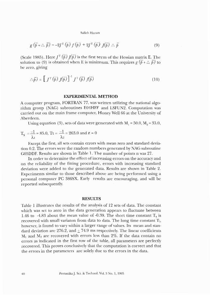
(9)

(Scale 1985). HereIf (f) j(f) is the first term of the Hessian matrix E. Thesolution to (9) is obtained when E is minimum. This requires g (f+ 6 f) tobe zero, giving

(10)

EXPERIMENTAL METHOD

A computer program, FORTRAN 77, was written utilizing the national algo­rithm group (NAG) subroutines E04HFF and LSFUN2. Computation wascarried out on the main frame computer, Honey Well 66 at the University ofAberdeen.

Using equation (3), sets of data were generated with M[ = 50.0, M2 = 35.0,

Ts = -1 = 85.0, Tt = -1 = 263.0 and E = 0AI 11.2

Except the first, all sets contain errors with mean zero and standard devia­tion 0.2. The errors were the random numbers generated by AG subroutineG05DDF. Results are shown in Table 1. The number of points n was 27.

In order to determine the effect of increasing errors on the accuracy andon the reliability of the fitting procedure, errors with increasing standarddeviation were added to the generated data. Results are shown in Table 2.Experiments similar to those described above are being performed using apersonal computer PC 386SX. Early results are encouraging, and will bereported subsequently.

RESULTS

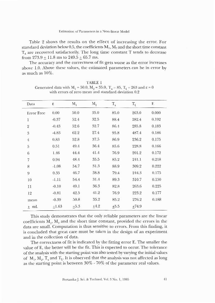
Table 1 illustrates the results of the analysis of 12 sets of data. The constantwhich was set to zero in the data generation appears to fluctuate between1.46 to -4.83 about the mean value of -0.39. The short time constant Ts isrecovered with small variaton from data to data. The long time constant T],however, is found to vary within a larger range of values. Its mean and stan­dard deviation are 276.2, and ± 74.9 ms respectively. The linear coefficientsM1 and M2 are recovered with errors less than 2%. If the data contain noerrors as indicated in the first row of the table, all parameters are perfectlyrecovered. This proves conclusively that the computation is correct and thatthe errors in the parameters are solely due to the errors in the data.

40 PertanikaJ. Sci. & Techno!. Vo!. 3 No.1, 1995

Estimation of Parameters in a Non-linear Model

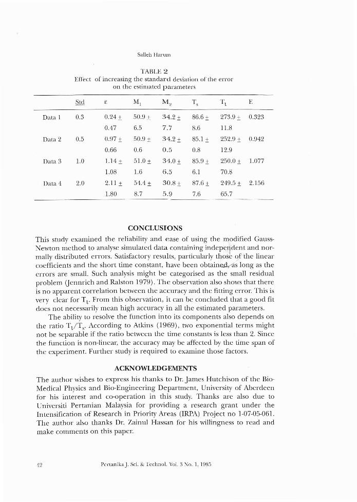
Table 2 shows the results on the effect of increasing the error. Forstandard deviation below 0.5, the coefficients M], M2 and the short time constantTs are recovered satisfactorily. The long time constant T tends to decreasefrom 273.9 ± 11.8 ms to 249.5 ± 65.7 ms.

The accuracy and the correctness of fit gets worse as the error increasesabove 1.0. Above these values, the estimated parameters can be in error byas much as 10%.

TABLE 1Generated data with M1 = 50.0, M2 = 35.0, Ts = 85, T1 = 263 and £ = 0

with errors of zero mean and standard deviation 0.2

Data £ M1 M2 Ts T1 E

Error Free 0.00 50.0 35.0 85.0 263.0 0.000

1 -0.37 52.4 32.5 88.4 282.4 0.192

2 -0.43 52.6 32.7 86.4 285.8 0.183

3 -4.83 62.2 27.4 95.8 487.4 0.186

4 0.83 52.8 37.5 86.9 236.2 0.175

5 0.51 49.4 36.4 85.6 228.8 0.166

6 1.46 44.4 41.4 76.9 201.2 0.172

7 0.94 48.4 35.5 85.2 241.1 0.218

8 -1.08 54.7 31.3 88.9 309.2 0.222

9 0.35 46.7 38.8 79.4 244.3 0.175

10 -1.11 54.4 31.4 89.3 310.7 0.150

11 -0.10 49.1 36.3 82.8 263.6 0.225

12 -0.81 42.5 41.2 76.9 223.2 0.177

mean -0.39 50.8 35.2 85.2 276.2 0.188

± std. ±1.63 ±5.3 ±4.2 ±5.5 ±74.9

This study demonstrates that the only reliable parameters are the linearcoefficients MI' M2 and the short time constant, provided the errors in thedata are small. Computation is thus sensitive to errors. From this finding, itis concluded that great care must be taken in the design of an experimentand in the collection of data.

The correctness of fit is indicated by the fitting error E. The smaller thevalue of E, the better will be the fit. This is expected to occur. The toleranceof the analysis with the starting point was also tested by varying the initial valuesof Mp M2, Ts and Tt . It is observed that the analysis was not affected as longas the starting point is between 30% - 70% of the parameter real values.

PertanikaJ. Sci. & Techno\. Vo\. ~ No.1, 1995 ..J-1

Salleh Harun

TABLE 2Effect of increasing the standard deviation of the error

on the estimated parameters

Std £ M1 M 2 Ts T 1 E

Data 1 0.3 0.24 ± 50.9 ± 34.2 ± 86.6 ± 273.9 ± 0.323

0.47 6.5 7.7 8.6 11.8

Data 2 0.5 0.97 ± 50.9 ± 34.2 ± 85.1 ± 252.9 ± 0.942

0.66 0.6 0.5 0.8 12.9

Data 3 1.0 1.14 ± 51.0 ± 34.0 ± 85.9 ± 250.0 ± 1.077

1.08 1.6 6.5 6.1 70.8

Data 4 2.0 2.11 ± 54.4 ± 30.8± 87.6± 249.5 ± 2.156

1.80 8.7 5.9 7.6 65.7

CONCLUSIONSThis study examined the reliability and ease of using the modified Gauss­Newton method to analyse simulated data containing independent and nor­mally distributed errors. Satisfactory results, particularly thos~ of the linearcoefficients and the short time constant, have been obtaine.dr-as long as theerrors are small. Such analysis might be categorised as the small residualproblem (Jennrich and Ralston 1979). The observation also shows that thereis no apparent correlation between the accuracy and the fitting error. This isvery clear for T l . From this observation, it can be concluded that a good fitdoes not necessarily mean high accuracy in all the estimated parameters.

The ability to resolve the function into its components also depends onthe ratio Tt/Ts' According to Atkins (1969), two exponential terms mightnot be separable if the ratio between the time constants is less than 2. Sincethe function is non-linear, the accuracy may be affected by the time span ofthe experiment. Further study is required to examine those factors.

ACKNOWLEDGEMENTSThe author wishes to express his thanks to Dr. James Hutchison of the Bio­Medical Physics and Bio-Engineering Department, University of Aberdeenfor his interest and co-operation in this study. Thanks are also due toUniversiti Pertanian Malaysia for providing a research grant under theIntensification of Research in Priority Areas (IRPA) Project no 1-07-05-06l.The author also thanks Dr. Zainul Hassan for his willingness to read andmake comments on this paper.

42 PertanikaJ. Sci. & Techno!. Vol. 3 No.1, 1995

Estimation of Parameters in a on-linear Model

REFERENCES

ATKINS, G.L. 1969. Multicompart'ment Modelfor Biological System. Methuen.

BEVINGTON, P.R. 1969. Data Reduction and En-or Analysis. Mc-Graw Hill.

GOODMAN, D.S. and R.P. aBLE. 1969. Turnover of plasma cholesterol in man. ] Clin.Invest. 47: 231-241.

JACQUEZ, j.A. 1972. System identification and inverse problem. In Compartmental Analysisin Biology and Medicine. p.l02-144. Elsevier.

JENNRICH, R.I. and M.L. R'\l~qON. 1979. Fitting nonlinear models to data. Ann. Rev.Biophys. Bio Engin. 8: 195-238.

LEIPERT, T.K. and D.W. MARQUART. 1976. Statistical analysis of NMR spin-lattice relaxationtime.]. Magn. Reson. 24: 184-199.

PHANG,j.M.M., G.A. BERMAN, R.M. FINERMAN, NEER and T.H. HAHN. 1969. Dietary pertur­bation of calcium metabolism in normal man: Compartmen tal analysis. .f. Clin. Invest.48: 67-77.

SCAI.E, L.E. 1985. Introduction to Non-linear Optimization. Macmillan.

PertanikaJ. Sci. & Technol. Vol. 3 No. 1,1995 43