assessing the mechanism of oil price fluctuation and ... · supply (ministry of trade...

Jurnal Ekonomi Malaysia 47(2) 2013 69 - 81

Assessing the Mechanism of Oil Price Fluctuation and Fiscal Policy Response in the Malaysian Economy

(Menilai Mekanisme Turun Naik Harga Minyak dan Tindak Balas Dasar Fiskal dalam Ekonomi Malaysia)

Nora Yusma Mohamed YusoffUniversity Tenaga Nasional (UNITEN)

ABSTRACT

The present paper analyzes the effects of oil price fluctuation on the economy;and fiscal policy response to the Malaysian economy. The data are analyzed utilizing a co-integration test, variance decomposition (VDC) and impulse response function (IRF) analysis under the unrestricted vector autoregression (VAR) methodology. The empirical findings of this study suggest that, in the short run, the Malaysia economy benefits from higher oil prices, as oil price shocks positively affect oil revenue. However, the real GDP of Malaysia is vulnerable to oil price fluctuations in the short term horizon. Meanwhile, oil price hikes exhibit an increasing trend for both GDP and total subsidy in the long run. Also, the results confirm that the changes in world oil prices have a significant short term impact on total government expenditure. These confirm that that fiscal policy is the main mechanism channel that determines the degree to which oil price shocks affect the economy. The study suggests that the adoption of expansionary fiscal policies during oil price shocks can facilitate rapid economic growth in the long run, as long as stable and persistent economic policies exist within the macroeconomic framework.

Keywords: Oil price shock; dynamic effect; fiscal policy;volatility; Malaysia

ABSTRAK

Kajian ini menganalisis kesan turun naik harga minyak dan tindak balas dasar fiskal dalam ekonomi Malaysia. Data dianalisis menggunakan analisis Variance Decomposition (VDC) dan Impulse Response Function (IRF) di bawah unrestricted autoregression vector (VAR) metodologi. Hasil kajian empirikal ini menunjukkan bahawa, dalam jangka masa pendek, ekonomi Malaysia menerima manfaat daripada kenaikan harga minyak yang tinggi, disebabkan kejutan harga minyak member kesan positif kepada hasil minyak. Walau bagaimanapun, KDNK sebenar Malaysia terdedah kepada turun naik harga minyak di dalam jangka masa pendek. Sementara itu, kenaikan harga minyak menunjukkan trend yang meningkat bagi kedua-dua KDNK dan jumlah subsidi untuk jangka masa panjang. Keputusan juga mengesahkan bahawa perubahan dalam harga minyak dunia mempunyai kesan jangka pendek yang besar ke atas jumlah perbelanjaan kerajaan. Ini mengesahkan bahawa dasar fiskal adalah saluran mekanisme utama yang menentukan sejauh mana kejutan harga minyak menjejaskan ekonomi. Kajian ini menunjukkan bahawa penggunaan dasar fiskal mengembang ketika kejutan harga minyak boleh meransang pertumbuhan ekonomi yang pesat untuk jangka masa panjang, selagi wujudnya dasar ekonomi yang stabil dan polisi yang konsisten dalam kerangka ekonomi makro.

Kata kunci: Kejutan harga minyak; kesan dinamik; dasar fiskal; turun naik; Malaysia

INTRODUCTION

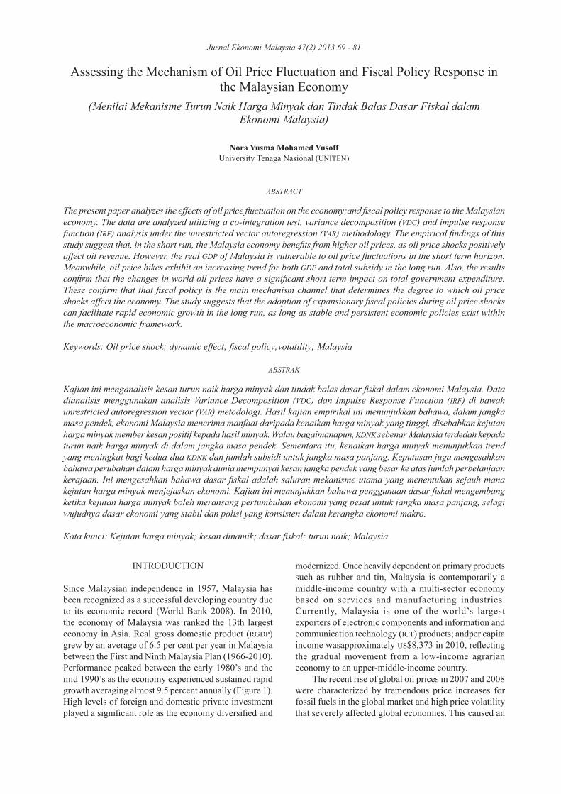
Since Malaysian independence in 1957, Malaysia has been recognized as a successful developing country due to its economic record (World Bank 2008). In 2010, the economy of Malaysia was ranked the 13th largest economy in Asia. Real gross domestic product (RGDP) grew by an average of 6.5 per cent per year in Malaysia between the First and Ninth Malaysia Plan (1966-2010). Performance peaked between the early 1980’s and the mid 1990’s as the economy experienced sustained rapid growth averaging almost 9.5 percent annually (Figure 1). High levels of foreign and domestic private investment played a significant role as the economy diversified and

modernized. Once heavily dependent on primary products such as rubber and tin, Malaysia is contemporarily a middle-income country with a multi-sector economy based on services and manufacturing industries. Currently, Malaysia is one of the world’s largest exporters of electronic components and information and communication technology (ICT) products; andper capita income wasapproximately US$8,373 in 2010, reflecting the gradual movement from a low-income agrarian economy to an upper-middle-income country.

The recent rise of global oil prices in 2007 and 2008 were characterized by tremendous price increases for fossil fuels in the global market and high price volatility that severely affected global economies. This caused an

70 Jurnal Ekonomi Malaysia 47(2)

intense global debate concerning energy security and the role of fossil fuels that were consequently linked to the issues to the rapid growth of global development (particularly in China and India) and climate change issues. The Malaysian economy is a small open economy with a large external trade sector. As such, the economy is more energy intensive in production and, hence, more sensitive to oil price increases. As a result, any price control or external price shock will ultimately be transmitted into the domestic economy. The price shocks have also given rise to political and economic instability (Al Amin et al. 2008).

As an oil exporting economy, higher world energy prices are expected to have a benefi cial impact on the Malaysian economy as the positive gains from higher oil prices could offset any negative impact on the Malaysian economy (e.g., through oil tax revenues, petroleum royalties, dividends and indirect tax revenues). This is accomplished through ‘pump priming’, whereby revenue from higher oil prices can be channeled back into the domestic economy through government expenditure channels.

Figure 1 shows that the annual revenue growth rate between 2000 and 2010 was, on average, 9.56 per cent, while the average expenditure growth rate was slightly lower than the average revenue growth rate of 9.2 percent. Nevertheless, the net impact of high oil prices on Malaysia’s economic performance also depends upon the exposure of the Malaysian economy to oil and the energy elasticity of demand, particularly in terms of domestic consumption particulars on energy consumption and the extent to which the spillover effect increases costs on other products and services. Although broad agreement exists that high oil prices have negative effects on macroeconomic variables, the magnitude and duration of the effects are uncertain.

Generally, when fuel prices increase, a spillover effect occurs within an economy in the form of increases in the costs on other products and services. As the price levels in an economy increase, the purchasing power and monetary wealth of households and businesses declines. The result is a decline in quantity of goods and

services demanded within the economy. Furthermore, high oil prices spread throughout the economy, driving up production and distribution costs on a wide variety of goods, which induces fi rms to reduce output. The situation, in turn, affects the number of laborers employed in the economy. The increase in production and distribution costs, which also puts pressure on the labor market, are caused by a number of factors,including a rise in the expected price level; workers demanding higher wages (wage push); and increases in non-labor inputs, such as raw materials (Frederic 2007). Although other factors are also important, high oil prices play a critical role in substantially reducing economic growth in most cases.

In the case of Malaysia, the price of electricity and petroleum products has been capped for almost 10 years. The Malaysian government has subsidizeds domestically produced liquefi ed natural gas (LNG) since January 1990; diesel since October 1999; and petrol since June 2005 (www.epu.gov.my). Since 1983, the retail price of petrol and diesel has been established using the Automatic Pricing Mechanism (APM) formula (www.epu.gov.my). The main objective of the APM is to stabilize the price of petrol and diesel in Malaysia to a certain extent through the use of a variable amount of sales tax and subsidy. As a result, the Malaysian government is able to set the retail price for petrol and diesel at a level where fl uctuations in the cost of the product will not affect the retail price. The APM ensures the difference between the retail price and the actual price is borne by subsidies and sales tax exemptions. Furthermore, the practice also standardizes the prices of fuel at pump stations; fi xes the margins of oil companies and dealers; ensures distribution channels are secure; and minimizes disruptions of the petrol and diesel supply (Ministry of Trade 2010).According to the Sales Tax Act 1972, the sales tax and subsidies are combined and the Malaysian government can collect a maximum sales tax of 58.62 cents per liter for petrol and 19.64 cents per liter for diesel. On the other hand, if the fi xed retail price is lower than the actual cost of the petrol and diesel at the pumps, the government can pay a subsidy of the same range. As of 2011, the Malaysian government has

FIGURE 1. Malaysia: Revenues, Expenditures, Real GDP and Defi cit, 2000-2010 (RM Billion)

71Assessing the Mechanism of Oil Price Fluctuation and Fiscal Policy Response in the Malaysian Economy

stated that it will reduce the maximum allowable subsidy of 58.62 sen per liter to a maximum subsidy of 30 sen per liter if needed. The new 30 senper litre maximum subsidy is as part of an improved APM that is designed to stabilize fuel retail prices and allow industry players to manage expenditures in a more orderly manner.

On the other hand, no doubt exists that the subsidy policies of the Malaysian government contributed to a large fiscal deficit, which has grown progressively from RM5 billion in 1998 to RM36.5 in 2008 and RM48 billion for 2009, which represents an average annual growth of 7 percent between 2000 and 2010 (Figure 1). Furthermore, in terms of sales tax lost, the foregone sales tax revenues due to the practice of fuel subsidization increased from an average of RM4.4 billion for the (2001-2003) period to RM7.15 billion in 2004, indicating that the foregone sales tax revenue grew at an average of 10 percent annually between 2001 and 2008 (EPU 2010). Moreover, if such subsidy policies were to continue, increasing global oil prices would trigger a reciprocal increase in the amount of government subsidies and sales tax exemptions on fuel and other essential goods and services in the economy. Hence, the Malaysian government’s expenditure will rise and non-oil tax revenues will fall, resulting in an increase in the Malaysian fiscal deficit or imbalance of current accounts. In regards to oil revenues, fuel subsidies accounted for 31.35% of oil revenues for the year 2005 and decreases to 12% and 11.5% for the years2008 and 2009, respectively. Figure 1 also shows that fuel subsidies increased sharply from 0.22% of RGDP for the year 2005 and rose to 0.36% by the year 2010.

Therefore, it cannot be denied that higher oil price shocks caused a substantial increase in Malaysian fuel subsidies. Thus, fuel subsidies put considerable pressure on the government budget,as well as resulting in revenue losses due to sales tax exemptions. Owing to these reasons, the Malaysian government committed to revising the retail price of fuel products and designing several fiscal policies to decrease the fiscal deficit. Thus, a series of gradual fuel subsidy removal policies were introduced by the Malaysian government in 2008. The purpose of the removal of the subsidies is to reduce the substantial increase in the amount of fuel subsidies and the revenue losses due to the sales tax exemption. Also, the gradual removal of fuel subsidies can help the Malaysian government to reduce the level of fossil energy use in the economy and support a shift to alternative green energy sources that may reduce carbon emissions in the environment. This, in turn, can support the ongoing commitment of the Malaysian government to the Kyoto Protocol II, which requires a voluntary reduction of up to 40 percent of emissions intensity of GDP in 2020.

Also, according to supply-side economics, lowering or eliminating subsidies to an appropriate level can reduce government burden and increase government revenues by transferring revenues back to the economy, which will result in faster economic growth. Supply-side economics

holds that a large increment in marginal income and capital gains tax rates to encourage the reallocation of income distribution via welfare redistribution will generate more income and produce more supply within the economy. The increased aggregate supply should result in decreasing prices and increased aggregate demand (Case & Fair 1999).

Thus, the findings of the present study concerning oil price shocksis crucial, as the study provides some valuable policy lessons regarding the importance of having well established frameworks for fiscal policy and inflation expectations. In this regard, the study explores the impact of symmetric oil price shocks on the Malaysian economy and simulates the effects of oil price shocks on RGDP, government expenditure and revenue in the Malaysian economy. The empirical findings of the present study are significant, particularly in relation to assisting governments and policy planners develop policy guidelines and designing proper fiscal policy instruments for planning at the macroeconomic level. Specifically, the present study assists in the assessment of the channel of higher oil prices transmitted to the rest economy and understanding how fiscal policy will respond to the shocks. In order to analyze the impacts of oil price shocks, the Generalised Impulse Response Function (GIRF) under the VAR model is employed. The VAR model is the most widely applied empirical approach for determining the relationship between oil prices and macroeconomic variables (Gronwald 2012).

The rest of this paper is discussed as follows. Section 2 briefly describes extant literature. Section 3 presents the data and methodology. Section 4 discusses the empirical results and findings. Section 5 discusses the policy implications. Section 6 offers a summary and concludes the present study.

LITERATURE REVIEW

The relationships between oil price shocks (positive and negative), economic growth and fiscal policy responses is well established in extant literature, as the findings regarding price impacts have important policy implications in future. Generally, positive oil price shocks, or higher oil prices, will increase price levels in an economy. As the price levels in an economy increase, the purchasing power and monetary wealth of households and businesses will decline, thus resulting in a decline in the quantity of goods and services demanded within an economy. Furthermore, high oil prices will then affect the economy as a whole, driving up production and distribution costs on a wide variety of goods, which will induce firms to reduce output (McConnell & Brue 2008). The reductions in output will also affect to the number of laborers employed in an economy. The increase in production and distribution costs are caused by various factors, including a rise in expected price levels; workers


demanding higher wages (wage push); and increases in non-labour inputs, such as raw materials,that puts further pressure on the labor market (Frederic 2007). Holding everything else constant, a decline in RGDP due to rising oil prices will result in a decline of tax base and, if tax rates are held constant, tax revenues will fall. Moreover, should oil prices continue to increase, the amount of government subsidies on fuel and other essential items will also increase. Thus, governmental expenditures will rise and tax revenues will fall, resulting in an increase in the fiscal deficit of a country.

On the other hand, many researchers argue that a negative correlation exists between increases in oil prices and the subsequent economic downturns in the United States (e.g., Hamilton 1983; Burbidge & Harrison 1984; Gisser & Goodwin 1986; Mork 1989; Hamilton 1996; Bernanke et al. 1997; Hamilton & Herrera 2001; and Hamilton 2003). Also, other studies find that strong correlations or co-integration relationships between higher world oil prices and macroeconomic variables exist in the long run (e.g., Hamilton 2003; Jones et al. 2004; Rodrigues & Sanchez 2004).

Lorde et al. (2009) find that oil prices are the major determinant of economic activity in the USA. Hutchison (1993) also finds that positive or increased in oil price shocks exert a negative impact on real gross national product (RGNP) growth and inflation variance in the USA and Japan. In the case of Korea, Glasure (2002) investigates the positive effect of oil price shocks on real national income in a non-oil producing country. The results confirm that positive oil price shocks affect real national income adversely. Zhang (2008) analyzes the asymmetric effect between oil price shocks and economic growth in Japan using a nonlinear approach. The empirical evidence confirms the existence of nonlinearity between these two variables. Negative oil price shocks (price decrease) tend to have a larger impact on economic growth rather than positive oil price shocks. Lardic and Mignon (2008) analyze the long-term relationship between oil prices; and economic activity and the GDP of the US, G-7, Europe and Euro economies. The results indicate that evidence exists of asymmetric co-integration between oil prices and GDP, but the standard co-integration was rejected.

In oil-importing countries, Mehrara (2008) confirms that oil revenue shocks tend to affect output in asymmetric and non-linear ways. The findings suggest that negative oil shocks affect output growth adversely, while positive shocks play a limited role in stimulating economic growth. However, Mehrara and Oskoui (2007) find that oil price shockis the main source of output fluctuations of oil-producing countries of Saudi Arabia and Iran, but not in Kuwait and Indonesia. Tan (2009) investigates the asymmetric impacts of crude oil price shocks on the Malaysian macro economy. The findings indicate that oil price shocks affect industrial output and inflation, while RGDP is vulnerable in the short term horizon. However, oil

price shocks on output are asymmetric, but not inflated. On the contrary, the response of terms-of-trade to oil price shocks is statistically insignificant. On the other hand, Mork (1989) finds asymmetry between the responses of the GDP and oil-price increases and decreases. The main conclusion reached is that the decrease is not statistically significant. Thus, Mork (1989) confirms that a negative correlation between GDP and increases in oil-price is persistent when data from 1985 onwards are included.

Lee and Ronald (1995) report that the response of the GDP to an oil-price shock depends greatly upon the environment of oil-price stability. An oil shock in a price stable environment is more likely to have greater effects on GDP than one in a price volatile environment. Abeysinghe (2001) concludes that high oil prices also adverse affect the economies of net-oil exporting countries. High oil prices dampen trade and hinder the economic growth of oil exporting trading partners.

DATA SOURCES AND METHODOLOGY

DATA SOURCES

Annual data for macroeconomic variables covering the period 1980-2010 is reused. Data concerning oil prices (OILP), RGDP, oil revenue (OR), non-oil revenue (NOR), government total expenditure (GOE) and total subsidy (SUB) macroeconomic variables are applied. The RGDP data are collected from the Department of Statistics, while the GOE, OR, NOR, SUB and OILP data are collected from the Economic Planning Unit (www.epu.gov.my). Furthermore, all variables are measured in constant price (2000 as a base year) and transformed into a logarithm base. Also, all time series data use logarithmic differences as a proxy for growing rates. This procedure ensures that all variables are stationary and reduces heteroskedasticity (Sari & Soytas 2006).

METHODOLOGY

The present study utilizes a co-integration test, the impulse response function (IRF) and variance decomposition (VDC) analysis under a vector auto-regression (VAR) framework. The co-integration procedure requires time series systems to be non-stationary in their levels. If a non-stationary series must be differenced d times to become stationary, then it is said to be integrated of order d (i.e., I (d)) (Engle and Granger 1987). For this reason, the properties of the variables are checked by the unit root test. In the present study, the Augmented Dickey Fuller (ADF) (Dickey & Fuller 1979) approaches are employed. Thus, the null and alternative hypothesis of unit root tests can be written as follows:

H0: α = 0 (Yt is non-stationary or there is a unit root).H1: α < 0 (Yt is stationary or non-unit root).


When both series are integrated in the same order, we can proceed to examine the presence of co-integration (Johansen & Juselius 1990). For this analysis, the Johansen and Juselius (1990) method is employed. The Johansen and Juselius (J-J) test, applies the maximum likehood procedures of the VAR model to determine the number of co-integrating vector.The J-J procedures specify two likehood ratio tests statistics, referred to as γtrace and γmax. Furthermore, the co-integration test is employed to investigate the long run equilibrium between the variables in the multivariate models. The analysis is based upon the following equations:

ln Yt = α0+ Σ βi ln Yt+ Σ χj ln Xt + εt (1)

ln Xt = γ20+ Σ σi ln Xt + Σ τj ln Yt + εt (2)

where (Yt , Xt) i.e. are dependence variables, εt is a random error term with mean zero, and βi and χj are the coefficient estimates for independent variables. To perform the co-integration test, the null hypothesis is created that no co-integration exists among the variables. The null hypothesis of no co-integration (r = 0) is rejected if trace statistics or maximal eigenvalues exceed the critical value,which means that coefficient values of independent variables is not equal to zero and co-integration exists between the two variables (i.e., Yt , Xt).

Having specified the model, the next step is to find the appropriate lag length of the co-integration.The results of co-integration tests are sensitive to the lag chosen (Hannan & Quinn 1978). The lag length chosen is based upon information provided by the selection of lag length information criteria (Ng and Perron 1995). In the present study, the Akaike information criterion (AIC); Schwarz information criterion (SIC); and Hannan-Quinn information criterio (H-Q) criteria are used to decide the number of lags, p. If p is too small, then the remaining serial correlation in the errors will bias the test. If p is too large, then the power of the test will suffer. Thus, the lag length is chosen that minimizes AIC, SIC and H-Q for the VAR model (Ng and Perron 1995). Once the order of the VAR is determined, a test for misspecification is performed. The Lagrange Multiplier (LM) test is employed for autocorrelation tests of the VAR residuals.

Next, the VAR is tested to confirm that it satisfies the stability condition. In the present study, the root of the AR Polynomial test is employed to confirm that no root lies outside the unit circle (Johansen & Juselius 1990). For a set of n time series variables, yt = (u1t, y2t, ..., ynt)´, and yt is stationary if all of the roots lie outside the unit circle. A VAR model of order p (VAR(p)) can be written as:

yt = A1yt–1 + A2yt–2 + ... + Apyt–p + ut (3)

where the Ai represents (n × n) coefficient matrices and ut = (u1t, u2t, ..., unt)´ is an unobservable i.i.d. zero mean error term. The stability of a VAR can be examined by calculating the roots of:

(In – A1L – A2L2 – ...) yt = A(L)yt (4)

The characteristic polynomial is defined as:

Π(z) = (In – A1z – A2z2 – ...) (5)

If the roots of |Π(z)| = 0, the results will provide the necessary information concerning the stationarity or nonstationarity of the process; and the hypothesis that no root lies outside the unit circle has been rejected. The necessary and sufficient condition for stability is that all characteristic roots lie outside the unit circle. If this is the case, Π is of full rank and all variables are stationary (Johansen & Juselius 1990).

The dynamic interactions between the world oil prices and macroeconomic variables are analyzed by the IRF and VDC, which are based upon the VAR system. The Generalized IRF (GIRF) procedures are applied to simulate a positive standard error unit shock on the current and future values of the variable. The result of the GIRF procedures are more robust compared to Cholesky decomposition and Orthogonalized IRF procedures, which are sensitive to the ordering of the variables (Gujarati 2010). Specifically, the GIRF test is used to determine the extent to which RGDP variables and components of fiscal policy respond to an oil price shock and to what extent such shocks are persistent.

MODEL SPECIFICATION

The dynamic interactions between world oil prices and macroeconomic variables are analyzed by the IRF and VDC, which are based upon the unrestricted VAR system. In order toestimate a VAR, each equation is estimated using the OLS method as follows:

RGDPt = α + Σ k

j=1 βRGDPt–j + Σ

k

j=1 γGOEt–j

+ Σk

j=1 ФORt–j + Σ

k

j=1 δNORt–j

+ Σk

j=1 φOILPt–j + Σ

k

j=1 ψOILPt–j + U1t (6)

GOEt = α + Σk

j=1 γGOEt–j + Σ

k

j=1 βRGDPt–j

+ Σk

j=1 ФORt–j + Σ

k

j=1 δNORt–j

+ Σk

j=1 φOILPt–j + Σ

k

j=1 ψOILPt–j + U2t (7)

Where, Ut = (U1t, U2t) is the stochastic error terms for t = 1, 2, ..., T. In addition, U1t and U2t are assumed independent and with zero mean,where E (U1t) = 0, k is the lag length criteria; α and α´ are constant terms; and β, γ and δ are the coefficient estimates for independent variables. The VAR model (Equations 3 and 4) is extended to comprise the 6 following major endogenous economic variables: OILP, RGDP, OR, NOR, SUB and GOE.


EMPIRICAL RESULTS AND FINDINGS

The ADF units-root test is performed for levels and the first differences for all variables, as depicted in Table 1. Table 1 shows that all variables have a unit root in their level, since the p-value for all series are not significant at all levels. Based on the estimated results, the null hypothesis of unit roots is not rejected even at the 10% significance level. However, when the ADF test is performed at first difference, the results indicate that all variables are I(1) since the P-values are significant at the 1% and 5% levels. The result indicates that after the first difference of all variables is obtained, no evidence exists concerning the existence of unit roots. ADF tests suggest that all variables appear to be integrated at an order of I(1) since the P-values are significant at the 1% and 5% levels. Hence, the variables in the models are qualified for inclusion in a long term equilibrium relationship.

Based on the ADF test, the Johansen-Julius (JJ) cointegration analysis is performed. The null hypothesis of r = 0 and r < 1 is rejected since the computed value (F-value) of the trace test is more than critical value at 1% and 5% level. Meanwhile, for max eigenvalue, the results indicate that the null hypothesis of r = 0 is rejected at at 1% and 5% level. The results presented in Table 2 show that the null hypothesis (no co-integration exists, r = 0), is clearly rejected since the trace statistics and maximal eigenvalue exceed the critical values at the 1% and 5% levels. Therefore, the resultsindicate that a long run relationship exists among the variables in the model. Furthermore, OILP, RGDP, OR, NOR, GOE and SUB, which are in log forms, are co-integrated and follow a common long run relationship.

Having specified the model, determining the appropriate lag length of the VAR model is the next step in the analysis. The AIC, H-Q and SBC criteria are employed

TABLE 1. Augmented Dickey Fuller (ADF) Unit Root Test results for Stationary

AT LEVEL First DifferencesConstant and No Trend Constant and Trend Constant and No Trend Constant and Trend

lags t-value Prob. lags t-value Prob. lags t-value Prob. lags t-value Prob.LOILP 0 0.334 0.9763 0 -1.11 0.9104 1 -4.19 0.0029*** 1 -5.46 0.0007***LGDP 0 -0.9835 0.7462 0 -1.145 0.9037 0 -4.38 0.0017*** 0 -4.37 0.0086***LSUB 0 -0.146 0.9351 0 -2.017 0.569 1 -4.21 0.0028*** 1 -4.99 0.0021***LGOE 3 2.674 1.00 0 -1.47 0.817 0 -5.90 0.000*** 2 -4.66 0.0048***LOR 0 0.13 0.9628 0 -1.722 0.7161 0 -5.65 0.0001*** 0 -5.81 0.0003***LNOR 0 -0.1254 0.9377 0 -1.964 0.5967 0 -5.78 0.000*** 0 -5.86 0.0002***

Notes: (1)***indicatesa significance level of 1%. (2) The optimum lags lengths for the ADF determined by the Schwarz Information Criterion (SIC).Source: Output of E-Views Package Version 7

TABLE 2. J-J Test for Cointegration Test

HypothesizedNo. of CE(s)

TraceStatistic

Critical Value 0.05 Prob. Maxi

EigenvalueCritical Value

0.05 Prob. Results

None* (r = 0) 117.73 95.75 0.0007*** 45.02 40.08 0.0128** Trace Test indicates 2 and max-eigenvalue indicates 1 cointegration equation at 1% and 5% level

At most 1 (r < 1) 72.71 69.82 0.0289** 29.35 33.88 0.1578At most 2 (r < 2) 43.35 47.86 0.1242 20.60 27.58 0.3008

At most 3 (r < 3) 22.75 29.80 0.2586 13.79 21.13 0.3822

Notes:*** and ** denote statistically significance at the 1% and 5% levels, respectively

TABLE 3. VAR Lag Order Selection Criteria

LAG LR FPE AIC SC HQ 0 NA 7.30e+10 42.04082 42.32630* 42.12809 1 72.17074* 3.28e+10* 41.17555* 43.17386 41.78645* 2 26.66716 1.08e+11 41.96917 45.68031 43.10370

* indicates the lag order selected by the criterion. LR refer to the sequential modified LR test statistic (each test at 5% level); FPE refers to thefinal prediction error; AIC refers to the Akaike information criterion; SC refers to the Schwarz information criterion; and HQ refers to the Hannan-Quinn information criterion


to select the optimal number of lags (Ng & Perron, 1995). Based on the minimum AIC criteria value, the results of lag 1 of the VAR model is chosen (see Table 3). Following the determination of the order of the VAR model, a test for misspecifi cation is performed.

Table 4 reports the results of the LM test for residual serial correlation. The results suggest that no obvious residual autocorrelation problems existed in the model since because all p-values are larger than the 0.05 level of signifi cance (Hanann & Quinn 1978). Additionally, the root of the AR polynomial test is employed for stability testing of the estimated VAR model.

-20

-10

0

10

20

30

1 2 3 4 5 6 7 8 9 10

Response of DOILP to Generalized OneS.D. DOILP Innovations

deviation (SD) symmetric OILP shocks tothe current and future values of endogenous variables. Estimations of the GIRFs are conducted 10 periods ahead for each endogenous variable based upon the VAR system, where decomposition values converge to stable states.

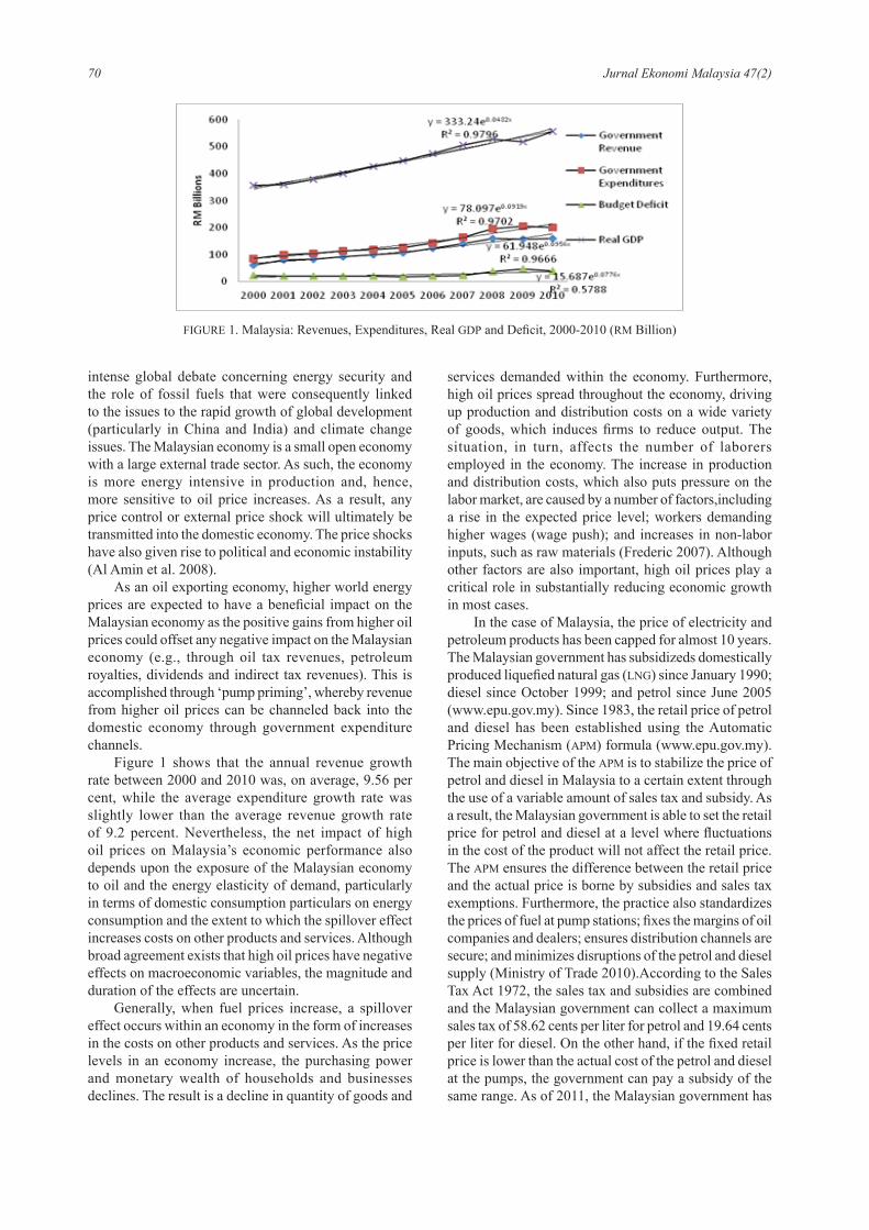
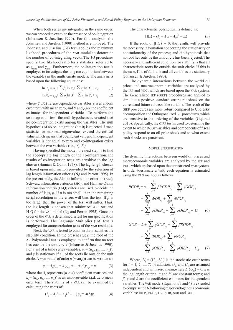
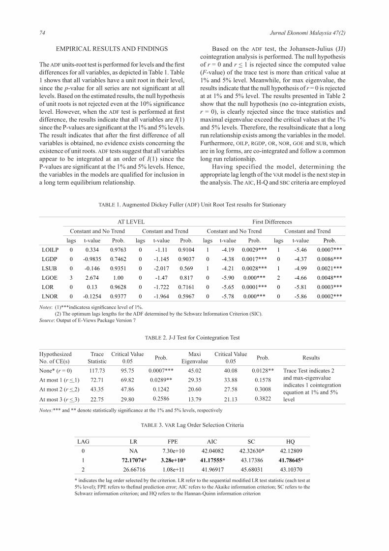
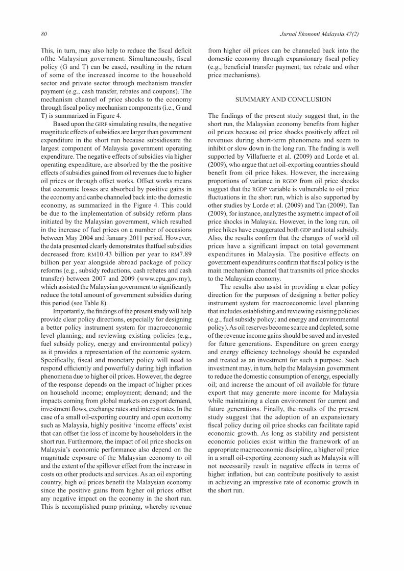
Figure 2 (a) shows the response pf OILP shocks to own shocks. Figure 2 (b) suggests that the OILP shock has an immediate effect, which leads to a decrease in RGDP in the short run. The larger negative impact occurs in the third period, which was approximately 0.15%. This was followed by a gradual increase over next periods until the fi fth period. However, the impact on RGDP growth becomes stable or asymptote to 0 after the sixth period. This suggests that the negative impact of OILP shock on the growth rate of GDP is relatively short-lived.

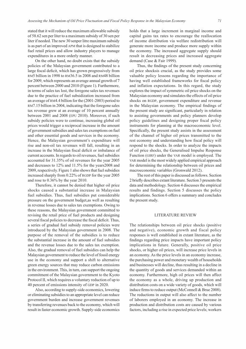
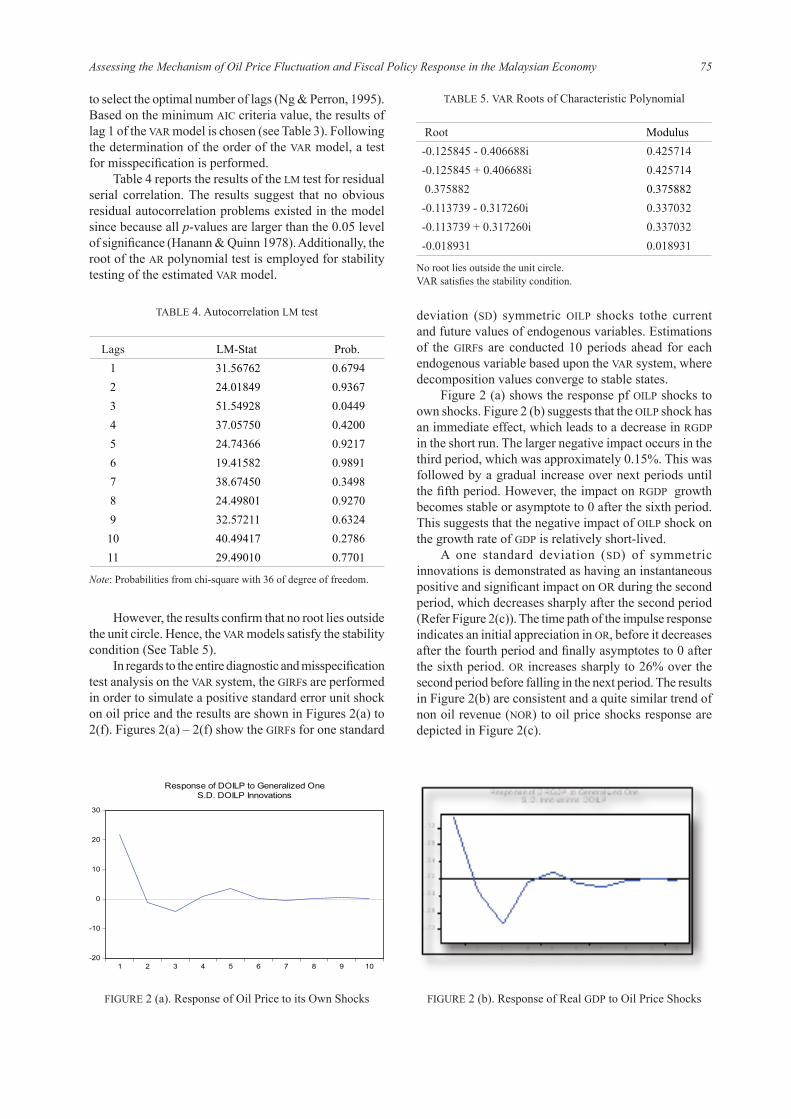
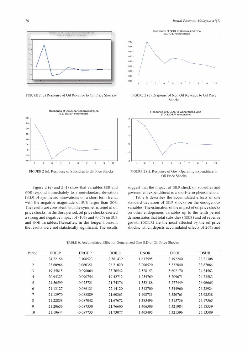
A one standard deviation (SD) of symmetric innovations is demonstrated as having an instantaneous positive and signifi cant impact on OR during the second period, which decreases sharply after the second period (Refer Figure 2(c)). The time path of the impulse response indicates an initial appreciation in OR, before it decreases after the fourth period and fi nally asymptotes to 0 after the sixth period. OR increases sharply to 26% over the second period before falling in the next period. The results in Figure 2(b) are consistent and a quite similar trend of non oil revenue (NOR) to oil price shocks response are depicted in Figure 2(c).

FIGURE 2 (a). Response of Oil Price to its Own Shocks FIGURE 2 (b). Response of Real GDP to Oil Price Shocks

TABLE 5. VAR Roots of Characteristic Polynomial

Root Modulus-0.125845 - 0.406688i 0.425714-0.125845 + 0.406688i 0.425714 0.375882 0.375882-0.113739 - 0.317260i 0.337032-0.113739 + 0.317260i 0.337032-0.018931 0.018931

No root lies outside the unit circle.VAR satisfi es the stability condition.

TABLE 4. Autocorrelation LM test

Lags LM-Stat Prob.1 31.56762 0.67942 24.01849 0.93673 51.54928 0.04494 37.05750 0.42005 24.74366 0.92176 19.41582 0.98917 38.67450 0.34988 24.49801 0.92709 32.57211 0.632410 40.49417 0.278611 29.49010 0.7701

Note: Probabilities from chi-square with 36 of degree of freedom.

However, the results confi rm that no root lies outside the unit circle. Hence, the VAR models satisfy the stability condition (See Table 5).

In regards to the entire diagnostic and misspecifi cation test analysis on the VAR system, the GIRFs are performed in order to simulate a positive standard error unit shock on oil price and the results are shown in Figures 2(a) to 2(f). Figures 2(a) – 2(f) show the GIRFs for one standard


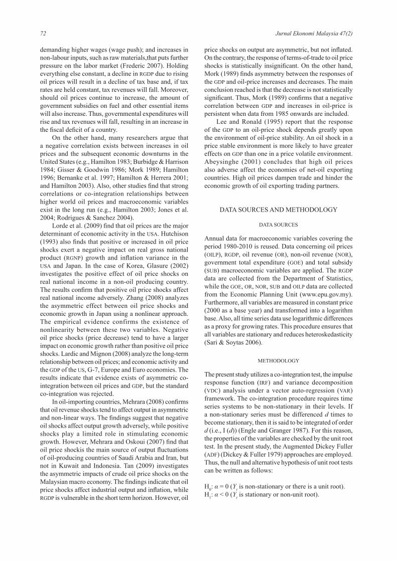
Figure 2 (e) and 2 (f) show that variables SUB and GOE respond immediately to a one-standard deviation (S.D) of symmetric innovations on a short term trend, with the negative magnitude of SUB larger than GOE. The results are consistent with the symmetric trend of oil price shocks. In the third period, oil price shocks exerted a strong and negative impact of -10% and -0.5% on SUB and GOE variables.Thereafter, in the longer horizon, the results were not statistically signifi cant. The results

suggest that the impact of OILP shock on subsidies and government expenditures is a short-term phenomenon.

Table 6 describes the accumulated effects of one standard deviation of OILP shocks on the endogenous variables. The estimation of the impact of oil price shocks on other endogenous variables up to the tenth period demonstrates that total subsidies (DSUB) and oil revenue growth (DOILR) are the most affected by the oil price shocks, which depicts accumulated effects of 26% and

.000

.004

.008

.012

.016

.020

.024

.028

.032

1 2 3 4 5 6 7 8 9 10

Response of NOR to Generalized OneS.D.OILP Innovations

FIGURE 2 (d).Response of Non Oil Revenue to Oil Price Shocks

FIGURE 2 (c).Response of Oil Revenue to Oil Price Shocksv

-2

-1

0

1

2

3

1 2 3 4 5 6 7 8 9 10

Response of DGOE to Generalized OneS.D. DOILP Innovations

-10

-5

0

5

10

15

20

25

30

1 2 3 4 5 6 7 8 9 10

Response of DSUB to Generalized OneS.D DOILP Innovations

FIGURE 2 (e). Response of Subsidies to Oil Pice Shocks FIGURE 2 (f). Response of Gov. Operating Expenditure to Oil Price Shocks

TABLE 6. Accumulated Effect of Generalized One S.D of Oil Price Shocks

Period DOILP DRGDP DOILR DNOR DGOE DSUB 1 24.22156 0.106523 2.581439 1.617595 3.192240 22.21308 2 23.60966 0.060351 28.21020 3.206520 5.332840 33.87064 3 19.35815 -0.090064 23.76542 2.528153 5.602170 24.24563 4 20.94323 -0.090754 19.42712 1.254769 5.209671 24.23583 5 21.56599 -0.075721 21.74376 1.352188 5.277449 26.96665 6 21.13127 -0.086131 22.14120 1.512700 5.344960 26.28924 7 21.13970 -0.088889 21.60363 1.408731 5.320761 25.92538 8 21.22858 -0.087042 21.67672 1.385496 5.315736 26.17565 9 21.20656 -0.087330 21.76600 1.406509 5.321984 26.18539 10 21.19644 -0.087733 21.73077 1.403495 5.321596 26.13589


22%, respectively. The accumulated effects results also imply that the oil price shocks adversely affect RGDP by -0.08%, which indicates that a 1 percent increase in oil prices slightly decreases RGDP by 0.08% over the next ten periods. At the same time, the accumulated response over ten periods for NOR was 1.4%, which is far smaller than the impact on OR. Meantime, the accumulated response for GOE over the ten periods is estimated to be 5.3%, which indicates that a 1% increase in OILP shocks contributes to an increase in the GOE by 5.3% over the next ten periods.

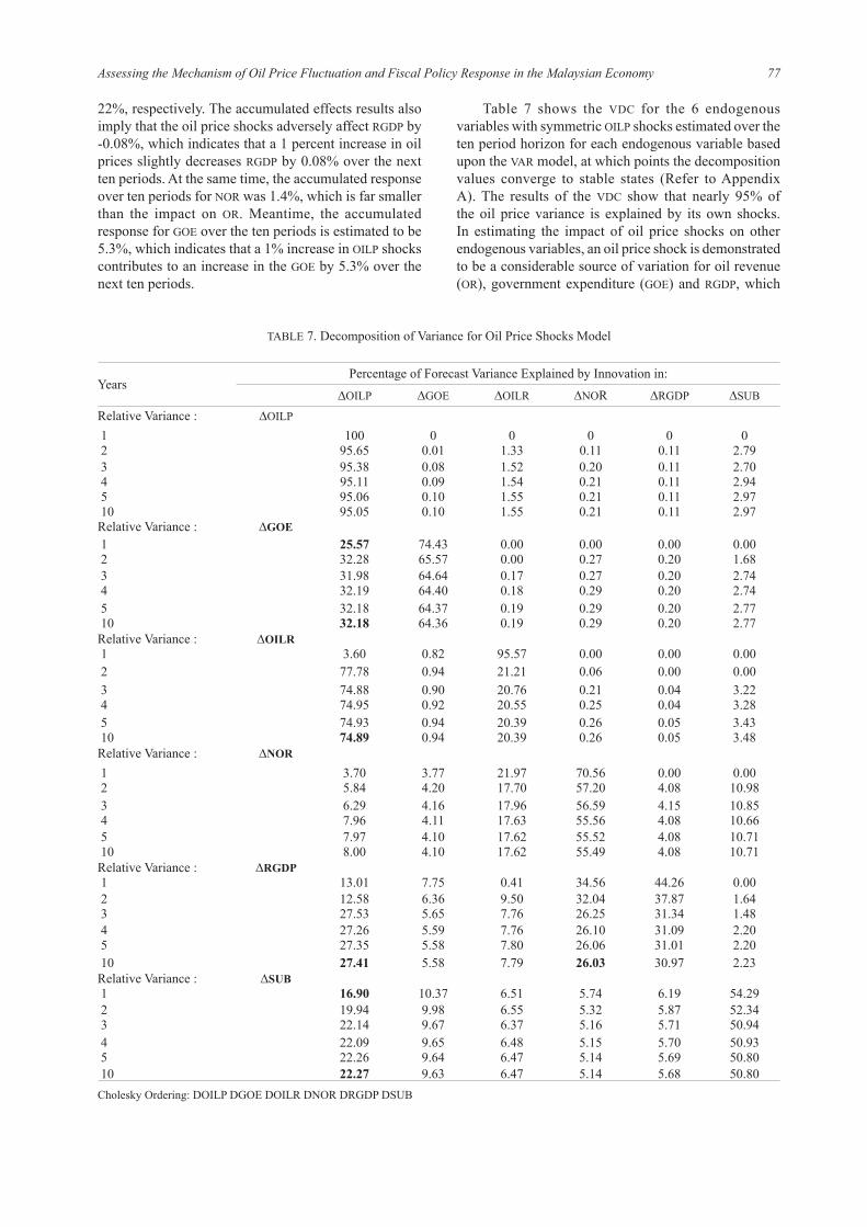
Table 7 shows the VDC for the 6 endogenous variables with symmetric OILP shocks estimated over the ten period horizon for each endogenous variable based upon the VAR model, at which points the decomposition values converge to stable states (Refer to Appendix A). The results of the VDC show that nearly 95% of the oil price variance is explained by its own shocks. In estimating the impact of oil price shocks on other endogenous variables, an oil price shock is demonstrated to be a considerable source of variation for oil revenue (OR), government expenditure (GOE) and RGDP, which

TABLE 7. Decomposition of Variance for Oil Price Shocks Model

YearsPercentage of Forecast Variance Explained by Innovation in:

∆OILP ∆GOE ∆OILR ∆NOR ∆RGDP ∆SUB

Relative Variance : ∆OILP 1 100 0 0 0 0 0 2 95.65 0.01 1.33 0.11 0.11 2.79 3 95.38 0.08 1.52 0.20 0.11 2.70 4 95.11 0.09 1.54 0.21 0.11 2.94 5 95.06 0.10 1.55 0.21 0.11 2.97 10 95.05 0.10 1.55 0.21 0.11 2.97Relative Variance : ∆GOE 1 25.57 74.43 0.00 0.00 0.00 0.00 2 32.28 65.57 0.00 0.27 0.20 1.68 3 31.98 64.64 0.17 0.27 0.20 2.74 4 32.19 64.40 0.18 0.29 0.20 2.74 5 32.18 64.37 0.19 0.29 0.20 2.77 10 32.18 64.36 0.19 0.29 0.20 2.77Relative Variance : ∆OILR 1 3.60 0.82 95.57 0.00 0.00 0.00 2 77.78 0.94 21.21 0.06 0.00 0.00 3 74.88 0.90 20.76 0.21 0.04 3.22 4 74.95 0.92 20.55 0.25 0.04 3.28 5 74.93 0.94 20.39 0.26 0.05 3.43 10 74.89 0.94 20.39 0.26 0.05 3.48Relative Variance : ∆NOR 1 3.70 3.77 21.97 70.56 0.00 0.00 2 5.84 4.20 17.70 57.20 4.08 10.98 3 6.29 4.16 17.96 56.59 4.15 10.85 4 7.96 4.11 17.63 55.56 4.08 10.66 5 7.97 4.10 17.62 55.52 4.08 10.71 10 8.00 4.10 17.62 55.49 4.08 10.71Relative Variance : ∆RGDP 1 13.01 7.75 0.41 34.56 44.26 0.00 2 12.58 6.36 9.50 32.04 37.87 1.64 3 27.53 5.65 7.76 26.25 31.34 1.48 4 27.26 5.59 7.76 26.10 31.09 2.20 5 27.35 5.58 7.80 26.06 31.01 2.20 10 27.41 5.58 7.79 26.03 30.97 2.23Relative Variance : ∆SUB 1 16.90 10.37 6.51 5.74 6.19 54.29 2 19.94 9.98 6.55 5.32 5.87 52.34 3 22.14 9.67 6.37 5.16 5.71 50.94 4 22.09 9.65 6.48 5.15 5.70 50.93 5 22.26 9.64 6.47 5.14 5.69 50.80 10 22.27 9.63 6.47 5.14 5.68 50.80Cholesky Ordering: DOILP DGOE DOILR DNOR DRGDP DSUB


accounts for 75%, 32% and 27.5% of the variation, respectively. On the other hand, non-oil revenue also contributes as much volatility to RGDP growth, which is around 26%. From the second period onwards, oil price shocks are also found to have a greater impact on GOE with variances ranging from 25% to 32%, followed by the RGDP and SUB with variances ranging from 12% to 27% and 20% to 22%, respectively. Importantly, oil price shocks exert a greater impact on RGDP growth during the second period, at which point volatility increases sharply from 12.58% to 27.5%.

POLICY IMPLICATIONS

The present study investigates the symmetric effects of oil price shock based upona one standard deviation (SD) of symmetric innovations ina small oil-exporting economy such as Malaysia. Yearly data is utilized for the (1980-2010) period. Cointegration tests, GIRF and VDC under a VAR model are used to estimate the oil price shocks on RGDP and following fi scal policy tools: government expenditure, oil revenue, non-oil revenue and total subsidy. The fi ndings suggest that the impact of symmetric oil price shocks has a direct and positive impact on oil revenue, even if a short-term phenomenon. This occurs because oil revenues constitute a large component of total government revenue, making fi scal policy directly sensitive to oil price changes.

As an oil exporting country, high oil prices in the short term benefi tted Malaysia oil income revenues, especially between 2005 and 2008 when crude oil prices increased sharply from USD57 to USD95 per barrel. Thus, volatility in crude oil prices (i.e. positive symmetric (high oil prices)) benefi cially impacts the Malaysia economy through oil revenues, as is the case other oil producing countries.The fi nding is well supported by Villafuerte

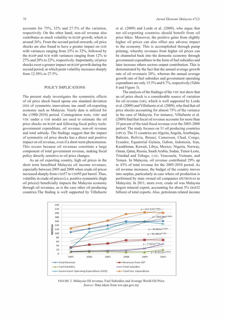
et al. (2009) and Lorde et al. (2009), who argue that net oil-exporting countries should benefit from oil price hikes. Moreover, the positive gains from slightly higher oil prices can also offset any adverse impact to the economy. This is accomplished through pump priming, whereby revenues from higher oil prices can be channeled back into the domestic economy through government expenditure in the form of fuel subsidies and later increase others sectors output contribution. This is demonstrated by the fact that the annual average growth rate of oil revenueis 28%, whereas the annual average growth rate of fuel subsidies and government operating expenditure are only 15.5% and 6.7%, respectively (Table 8 and Figure 3).

The analysis of the fi ndings of the VDC test show that an oil price shock is a considerable source of variation for oil revenue (OR), which is well supported by Lorde et al. (2009) and Villafuerte et al. (2009), who fi nd that oil price shocks accounting for almost 75% of the variance in the case of Malaysia. For instance, Villafuerte et al. (2009) fi nd that fi scal oil revenue accounts for more than 25 percent of the total fi scal revenue over the 2005-2008 period. The study focuses on 31 oil producing countries (OPCs). The 31 countries are Algeria, Angola, Azerbaijan, Bahrain, Bolivia, Brunei, Cameroon, Chad, Congo, Ecuador, Equatorial Guinea, Gabon, Indonesia, Iran, Kazakhstan, Kuwait, Libya, Mexico, Nigeria, Norway, Oman, Qatar, Russia, Saudi Arabia, Sudan, Timor-Leste, Trinidad and Tobago, UAE, Venezuela, Vietnam, and Yemen. In Malaysia, oil revenue contributed 29% up to 43% of total revenue for the 2005-2010 period. As oil revenue increases, the budget of the country moves into surplus, particularly in case where oil production is performed by state owned oil companies (PETRONAS in Malaysia). In 2011, more over, crude oil was Malaysia largest mineral export, accounting for about 5% (RM32 billion) of total exports. Also, petroleum related income

FIGURE 3. Malaysia Oil revenue, Fuel Subsidies and Average World Oil PriceSource: Data taken from ww.epu.gov.my


is the largest single contributor to government revenue in 2011, accounting for approximately 33.9% (RM62.9 billion) of the total revenue of the Malaysian government (www.epu.gov.my). In 2009, the contribution of petroleum-related income to total government revenue reached its highest level (almost 40% or RM68.8 billion) (Table 8). The positive income of oil revenue helps to improve the current account balance as well as narrow the deficit gap for the Malaysian budget.

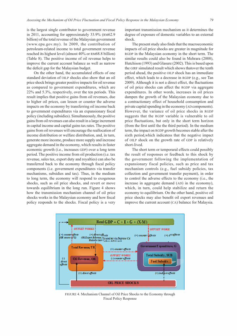
On the other hand, the accumulated effects of one standard deviation of OILP shocks also show that an oil price shock brings greater positive impacts for oil revenue as compared to government expenditures, which are 22% and 5.3%, respectively, over the ten periods. This result implies that positive gains from oil revenues, due to higher oil prices, can lessen or counter the adverse impacts on the economy by transferring oil income back to government expenditures via an expansionary fiscal policy (including subsidies). Simultaneously, the positive gains from oil revenues can also result in a large increment in capital income and capital gains tax rates. The positive gains from oil revenues will encourage the reallocation of income distribution or welfare distribution, and, in turn, generate more income, produce more supply and increase aggregate demand in the economy, which results in faster economic growth (i.e., increases GDP) over a long term period. The positive income from oil production (i.e. tax revenue, sales tax, export duty and royalties) can also be transferred back to the economy through fiscal policy components (i.e. government expenditures via transfer mechanisms, subsidies and tax). Thus, in the medium to long term, the economy will respond to exogenous shocks, such as oil price shocks, and revert or move towards equilibrium in the long run. Figure 4 shows how the transmission mechanism channel of oil price shocks works in the Malaysian economy and how fiscal policy responds to the shocks. Fiscal policy is a very

important transmission mechanism as it determines the degree of exposure of domestic variables to an external shock.

The present study also finds that the macroeconomic impacts of oil price shocks are greater in magnitude for RGDP in the Malaysian economy in the short term. The similar results could also be found in Mehrara (2008), Hutchison (1993) and Glasure (2002). This is based upon the GIRF simulated result which shows thatover the tenth period ahead, the positive OILP shock has an immediate effect, which leads to a decrease in RGDP (e.g., see Tan 2009). Although it is not a direct effect, the fluctuations of oil price shocks can affect the RGDP via aggregate expenditures. In other words, increases in oil prices dampen the growth of the Malaysian economy due to a contractionary effect of household consumption and private capital spending in the economy (AD components). However, the variance of oil price shocks in RGDP suggests that the RGDP variable is vulnerable to oil price fluctuations, but only in the short term horizon (from the first until the the third period). In the medium term, the impact on RGDP growth becomes stable after the sixth period,which indicatess that the negative impact of OILP shock on the growth rate of GDP is relatively short-lived.

The short term or temporaral effects could possibly the result of responses or feedback to this shock by the government following the implementation of expansionary fiscal policies, such as price and tax mechanism controls (e.g., fuel subsidy policies, tax collection and government transfer payment), in order to control the adverse effects to the economy (i.e., the increase in aggregate demand (AD) in the economy), which, in turn, could help stabilize and return the economy to equilibrium. On the other hand, positive oil price shocks may also benefit oil export revenues and improve the current account (CA) balance for Malaysia.

FIGURE 4. Mechanism Channel of Oil Price Shocks to the Economy through Fiscal Policy Response


This, in turn, may also help to reduce the fiscal deficit ofthe Malaysian government. Simultaneously, fiscal policy (G and T) can be eased, resulting in the return of some of the increased income to the household sector and private sector through mechanism transfer payment (e.g., cash transfer, rebates and coupons). The mechanism channel of price shocks to the economy through fiscal policy mechanism components (i.e., G and T) is summarized in Figure 4.

Based upon the GIRF simulating results, the negative magnitude effects of subsidies are larger than government expenditure in the short run because subsidiesare the largest component of Malaysia government operating expenditure. The negative effects of subsidies via higher operating expenditure, are absorbed by the the positive effects of subsidies gained from oil revenues due to higher oil prices or through offset works. Offset works means that economic losses are absorbed by positive gains in the economy and canbe channeled back into the domestic economy, as summarized in the Figure 4. This could be due to the implementation of subsidy reform plans initiated by the Malaysian government, which resulted in the increase of fuel prices on a number of occasions between May 2004 and January 2011 period. However, the data presented clearly demonstrates thatfuel subsidies decreased from RM10.43 billion per year to RM7.89 billion per year alongside abroad package of policy reforms (e.g., subsidy reductions, cash rebates and cash transfer) between 2007 and 2009 (www.epu.gov.my), which assisted the Malaysian government to significantly reduce the total amount of government subsidies during this period (see Table 8).

Importantly, the findings of the present study will help provide clear policy directions, especially for designing a better policy instrument system for macroeconomic level planning; and reviewing existing policies (e.g., fuel subsidy policy, energy and environmental policy) as it provides a representation of the economic system. Specifically, fiscal and monetary policy will need to respond efficiently and powerfully during high inflation phenomena due to higher oil prices. However, the degree of the response depends on the impact of higher prices on household income; employment; demand; and the impacts coming from global markets on export demand, investment flows, exchange rates and interest rates. In the case of a small oil-exporting country and open economy such as Malaysia, highly positive ‘income effects’ exist that can offset the loss of income by householders in the short run. Furthermore, the impact of oil price shocks on Malaysia’s economic performance also depend on the magnitude exposure of the Malaysian economy to oil and the extent of the spillover effect from the increase in costs on other products and services. As an oil exporting country, high oil prices benefit the Malaysian economy since the positive gains from higher oil prices offset any negative impact on the economy in the short run. This is accomplished pump priming, whereby revenue

from higher oil prices can be channeled back into the domestic economy through expansionary fiscal policy (e.g., beneficial transfer payment, tax rebate and other price mechanisms).

SUMMARY AND CONCLUSION

The findings of the present study suggest that, in the short run, the Malaysian economy benefits from higher oil prices because oil price shocks positively affect oil revenues during short-term phenomena and seem to inhibit or slow down in the long run. The finding is well supported by Villafuerte et al. (2009) and Lorde et al. (2009), who argue that net oil-exporting countries should benefit from oil price hikes. However, the increasing proportions of variance in RGDP from oil price shocks suggest that the RGDP variable is vulnerable to oil price fluctuations in the short run, which is also supported by other studies by Lorde et al. (2009) and Tan (2009). Tan (2009), for instance, analyzes the asymetric impact of oil price shocks in Malaysia. However, in the long run, oil price hikes have exaggerated both GDP and total subsidy. Also, the results confirm that the changes of world oil prices have a significant impact on total government expenditures in Malaysia. The positive effects on government expenditures confirm that fiscal policy is the main mechanism channel that transmits oil price shocks to the Malaysian economy.

The results also assist in providing a clear policy direction for the purposes of designing a better policy instrument system for macroeconomic level planning that includes establishing and reviewing existing policies (e.g., fuel subsidy policy; and energy and environmental policy). As oil reserves become scarce and depleted, some of the revenue income gains should be saved and invested for future generations. Expenditure on green energy and energy efficiency technology should be expanded and treated as an investment for such a purpose. Such investment may, in turn, help the Malaysian government to reduce the domestic consumption of energy, especially oil; and increase the amount of oil available for future export that may generate more income for Malaysia while maintaining a clean environment for current and future generations. Finally, the results of the present study suggest that the adoption of an expansionary fiscal policy during oil price shocks can facilitate rapid economic growth. As long as stability and persistent economic policies exist within the framework of an appropriate macroeconomic discipline, a higher oil price in a small oil-exporting economy such as Malaysia will not necessarily result in negative effects in terms of higher inflation, but can contribute positively to assist in achieving an impressive rate of economic growth in the short run.


REFERENCES

Abeysinghe, T. 2001. Estimation of direct and indirect impact of oil prices on growth. Economic Letters 73: 147-153.

Bernanke, B. S., Mark, G. & Mark, W. 1997. Systematic monetary policy and the effects of oil price shocks. Brookings Papers on Economic Activity 1: 91-124.

Burbidge, J. &Alan, H. 1984. Testing for the effects of oil-price rises using vector auto regressions. International Economic Review 25: 459-484.

Case, K. E. & Fair, R. C. 1999. Principles of Economics. 5th edition. New Jersey: Prentice-Hall.

Dickey, D. & Fuller, W. 1979. Distribution of the estimators for autoregressive time series with a unit root. Journal of American Statistical Association 74: 427-431.

Economic Planning Unit. 2010. Annual report (2010). Retrieved from hhtp://www.epu.com.my.

Frederic, M. 1997. Strategies for controlling inflation. National Bureau of Economic Research, NBER working paper series. Cambridge.

Gronwald, M. 2012. Oil and U.S. economy: A reinvestigation using rolling impulse response. The Energy Journal 4: 143-160.

Gujarati, D. 2003. Basic Econometrics. 4th edition. London: McGraw-Hill.

Hamilton J. D. 2003. What is an oil shock? Journal of Econometrics 113(2): 363-398.

Hamilton J. D. & Herrera, A. M. 2001. Oil Shocks and Aggregate Macroeconomic Behaviour: The Role of Monetary Policy. Discussion Paper 2001-10. University of California, San Diego.

Hamilton, J. D. 1983. Oil and the macroeconomy since World War II. Journal of Political Science 91: 228-248.

Hannan, E. J. & Quinn, B. G. 1978. The determination of the lag length of an autoregression. Journal of Royal Statistical Society 41: 190-195

Hutchison, M. 1993. Structural change and the macroeconomic effects of oil shocks: empirical evidence from the United States and Japan. Journal of International Money and Finance 12(6): 587-606.

International Energy Ascociation. 1999. World Energy Outlook 1999: Looking at Energy Subsidies – Getting the Prices Right. International Energy Agency: Paris.

Jones, D. W., Leiby, P. N. & Paik, I. K. 2002. Oil Price Shocks and the Macroeconomy: What Has Been Learned since 1996? In: Proceedings of the 25th Annual IAEE International Conference, Aberdeen, Scotland, June 26-29, 2002.

Johansen, S. & Juselius, K. 1990. Maximum likehood estimation and inference on co-integration with applications to the demand for money. Oxford Bulletin of Economics and Statistics 52: 169-210.

Lardic, S. & Valerie, M. 2008. Oil prices and economic activity: An asymmetric cointegration approach. Energy Economics 30(3): 847-855.

Lorde, T., Mahalia, J. & Chrystol, T. (2009). The macroeconomic effects of oil price fluctuations on a small open oil-producing country: The case of Trinidad and Tobago. Energy Policy. http://yadda.icm.edu.pl/yadda/element/bwmeta1.

Lee, K. & Ronald A. R. 1995. Oil shocks and the macroeconomy: The role of price variability. Energy Journal 16: 39-56.

McConnell, C. & Brue, S. 2005. Economics: Principles, Problems and Policies. 16th edition. New York: McGraw-Hill.

Mehrara, M. 2008. The asymmetric relationship between oil revenues and economic activities: the case of oil-exporting countries. Energy Policy 36(3): 1164-1168.

Ministry of Finance. 2010. Annual Reports of 2010. Kuala Lumpur: Malaysia Printing Office.

Ng, S. & Perron, P. 1995. Unit Root Tests in ARMA models with data-dependent methods for the selection of the truncation lag. Journal of the American Statistical Association 90: 268-281.

Mork, K. A. 1989. Oil and the macroeconomy when prices go up and down: An extension of Hamilton’s Results. Journal of Political Economy 91: 740-744.

Pesaran, H. H. & Shin, Y. 1998. Generalized impulse response analysis in linear multivariate models. Economic Letters 58: 17-29.

Rodriguez, R. & Sanchez, M. 2004. Oil price shocks and real GDP growth: Empirical evidence for some OECD countries. European Central Bank Working Paper 362.

Sari, R. & Soytas, U. 2006. The relationship between stock returns, crude oil prices, interest rates, and output: Evidence from a developing economy. Empirical Economics Letters 5(4): 205-220.

Tan, J. H. 2012. The effects of oil price shocks on output, inflation and terms-of-trade: Evidence for Malaysia. Journal of Business Management 2(1): 63-74.

Villafuerte, M. & Murphy, P. L. 2009. Fiscal policy in oil producing countries during the recent oil price cycle. IMF Working Paper 6.

World Bank. 2008. Climate Change and the World Bank Group: Phase I: An Evaluation of World Bank Win-Win Energy Policy Reforms. Washington, D. C.: World Bank.

Zhang, D. 2008. Oil shock and economic growth in Japan: a nonlinear approach. Energy Economics 30(5): 2374-2390.

Nora Yusma Mohamed YusoffDepartment Finance and EconomicsCollege of Business Management and Accounting University Tenaga Nasional (UNITEN)26700 Muadzam Shah Pahang Darul [email protected]

assessing the mechanism of oil price fluctuation and ... · supply (ministry of trade...

Documents