i

VOT 74158

THE INTEGRATION OF GLOBAL POSITIONING SYSTEM (GPS) AND METEOROLOGICAL OBSERVATIONS FOR TROPOSPHERIC MODEL

DEVELOPMENT IN MALAYSIAN REGION

(INTEGRASI SISTEM PENENTUDUKAN SEJAGAT (GPS) DAN CERAPAN METEOROLOGI BAGI PEMBANGUNAN MODEL TROPOSFERA DALAM

WILAYAH MALAYSIA)

MD. NOR KAMARUDIN WAN ABDUL AZIZ WAN MOHD AKIB

MOHAMAD SAUPI CHE AWANG MOHD ZAHLAN MOHD ZAKI

MUSTAFA DIN SUBARI

RESEARCH VOTE NO: 74158

Jabatan Kejuruteraan Geomatik Fakulti Kejuruteraan dan Sains Geoinformasi

Universiti Teknologi Malaysia

2006

ii

UTM/RMC/F/0024 (1998)

Lampiran 20

UNIVERSITI TEKNOLOGI MALAYSIA

BORANG PLAPORAN AKHI

TAJUK PROJEK : THE INTEGRATION O AND METEOROLOGI

MODEL DEVELOPME

(INTEGRASI SISTEM CERAPAN METEOR

TROPOSFERA DAL

Saya _ MD. NOR B

Mengaku membenarkan Laporan Akhir PeUniversiti Teknologi Malaysia dengan syara

1. Laporan Akhir Penyelidikan ini adalah

2. Perpustakaan Universiti Teknologi tujuan rujukan sahaja.

3. Perpustakaan dibenarkan mem

Penyelidikan ini bagi kategori TIDAK

4. * Sila tandakan ( / )

SULIT (Mengandun Kepentingan AKTA RAH TERHAD (Mengandun Organisasi/ TIDAK TERHAD

ENGESAHAN R PENYELIDIKAN

F GLOBAL POSITIONING SYSTEM (GPS) CAL OBSERVATIONS FOR TROPOSPHERIC NT IN MALAYSIAN REGION PENENTUDUKAN SEJAGAT (GPS) DAN OLOGI BAGI PEMBANGUNAN MODEL

AM WILAYAH MALAYSIA)

IN KAMARUDIN

nyelidikan ini disimpan di Perpustakaan t-syarat kegunaan seperti berikut :

hakmilik Universiti Teknologi Malaysia.

Malaysia dibenarkan membuat salinan untuk

buat penjualan salinan Laporan Akhir TERHAD.

gi maklumat yang berdarjah keselamatan atau Malaysia seperti yang termaktub di dalam SIA RASMI 1972).

gi maklumat TERHAD yang telah ditentukan oleh badan di mana penyelidikan dijalankan).

TANDATANGAN KETUA PENYELIDIK

Nama & Cop Ketua Penyelidik

Tarikh :

CATATAN : * Jika Laporan Akhir Penyelidikan ini SULIT atau TERHAD, sila lampirkan surat daripada pihak berkuasa/organisasi berkenaan dengan menyatakan sekali sebab dan tempoh laporan ini perlu dikelaskan

iii

ABSTRACT

(keywords: Global Positioning System (GPS), troposphere, meteorological data) The use of satellite based Global Positioning System (GPS) is normal in engineering and

surveying for a wide range of applications as the accuracy capability increases. Global

Positioning System (GPS) satellites provide precise all weather global navigation information

to users equipped with GPS receivers on or near the earth’s surface. The GPS satellites

transmit signals that are received by the receivers on the earth’s surface to determine the

position. The effects of other different error sources on the computed position have to be

removed from the data. The principal limiting error source is incorrect modeling of the delay

experienced by GPS signal propagating through the electrically neutral atmosphere, usually

referred to as the tropospheric delay.

The integration of ground based meteorological observations and GPS lead to a better

understanding of the tropospheric delay to the GPS signal and improve the GPS height

accuracy. The study conducted by integrating the Malaysian Active GPS Station (MASS)

data and ground based meteorological observations to analyze the variation occur to the GPS

height determination due to the tropospheric delay. The introduction of the Saastamoinen

tropospheric model to the data shows a delay variation for up to 20 meter in pseudorange

which causes an error up to 5 meter of height component. Processing with certain

tropospheric delay correction model using synchronizes ground meteorological and GPS data

at the same point can provide better accurate baseline.

iv

ABSTRAK

(katakunci: Global Positioning System (GPS), data kajicuaca (meteorology),troposfera) Penggunaan teknik Global Positioning System (GPS) berasaskan satelit adalah meluas dalam

kerja kejuruteraan dan pengukuran yang memerlukan kejituan tinggi. Satelit GPS

memberikan informasi navigasi global berkejituan tinggi sepanjang masa kepada pengguna

yang mempunyai alat penerima GPS di atas atau hampir permukaan bumi. Isyarat yang

dipancarkan oleh satelit GPS akan diterima oleh alat penerima GPS untuk penentuan

kedudukan. Walau bagaimana pun kesan dari sumber ralat ralat yang terdapat dalam

pengukuran perlu dihapuskan semasa pemprosesan pada data. Sabagai contoh, kesilapan

memodelkan kelewatan isyarat GPS yang melalui atmosfera bumi adalah salah satu daripada

ralat utama yang juga di kenali sabagai kelewatan troposfera.

Integrasi cerapan meteorologi dan GPS memberikan kefahaman yang jelas mengenai

kelewatan troposfera. Kajian yang dilaksanakan mengabungkan data daripada stesen MASS

(Malaysian Active GPS Station) dan cerapan meteorologi untuk menganalisis perubahan

ketinggian GPS disebabkan oleh kelewatan troposfera. Model troposfera Saastamoinen yang

di kenakan kepada data menunjukkan ralat sehingga 20 meter bagi data pseudorange. Ianya

menyamai ralat sehingga 5 meter bagi komponen ketinggian. Pemprosesan menggunakan

model kelewatan troposfera yang serasi berserta data meteorologi dan GPS pada titik tertentu

dapat meningkatkan kejituan pengukuran garis dasar.

v

vi

ACKNOWLEDGEMENTS

Allhamdulilah. First and foremost I would like to acknowledge the helpful and abundant

support of my research team: Assoc. Prof Dr. Wan Abdul Aziz Wan Mohd Akib, Assoc.

Prof. Dr Mustafa Din Subari, Mohd Zahlan Mohd Zaki and Mohamad Saupi Che Awang.

Their work, suggestions and discussions towards the completion of this research always

benefit my research.

I would also like to thanks the technical staffs of the Geomatic Engineering Department,

Faculty of Geoinformation Sciences and Engineering, UTM: Zulkarnaini Mat Amin, Zuber

Che Tak, Ramli Mohd Amin and Ajis Ahmad for their contribution in the research and

other that directly or indirectly help to make this research successful..

Not forgetting to my wife Zainariah Zainal and my sons Muhamad Elyas and Muhamad

Hanif for their understanding and support for me to carry out this research.

Lastly I would to thanks the government of Malaysia through the Ministry of Science,

Technology and Innovation (MOSTI) for supporting this research grant and to the Research

Management Centre (RMC), Universiti Teknologi Malaysia for the management and

administration of the fund.

vii

viii

TABLE OF CONTENTS

Page

TITLE i

DECLARATION ii

ABSTRACT iii

ABSTRAK iv

DICLOSURE FORM v

ACKNOWLEDGEMENT vi

TABLE OF CONTENTS viii

LIST OF FIGURES xii

LIST OF TABLES xiv

CHAPTER 1

INTRODUCTION 1.0 Overview 2

1.1 The Current State of Measuring Atmospheric Water Vapor 3

1.2 Problem Statement 6

1.3 Objectives 7

1.4 Scope of Research 7

1.5 Contribution 8

1.6 Outline Treatment 9

CHAPTER 2

THE APPLICATION OF GNSS FOR ATMOSPHERIC STUDIES IN

MALAYSIA Abstract 13

2.0 Introduction 14 2.1 Total Electron Content (TEC) from GPS 14

ix

2.2 Application in Atmospheric Studies 16

2.2.1 Universiti Teknologi Malaysia 16

2.2.2 Universiti Kebangsaan Malaysia 18

2.2.3 STRIDE Ministry of Defence 19

2.4 Conclusion 22

2.5 References 22

CHAPTER 3

EFFECTS OF TROPOSPHERIC ZENITH DELAY IN

SINGLE BASELINE DETERMINATION

Abstract 25

3.0 Introduction 26

3.1 Background 26

3.1.1 The Atmospheric Effects on GPS Signals 26

3.1.2 GPS Error Budget 27

3.1.3 Residual Atmospheric Effects 28

3.1.4 The Correction Methods 28

3.2 The experiments 30

3.2.1 The Data 30

3.2.2 MASS Data 30

3.2.3 Baseline 30

3.2.4 Surface Meteorological Data 31

3.2.5 IGS data 31

3.3 Processing 31

3.3.1 The Model 32

3.3.2 Ionospheric Free Solution 32

3.4 Data Analysis 33

x

3.5 Conclusion and Recommendation 37

3.6 Acknowledgements 38

3.7 References 38

3.8 Appendix 39

CHAPTER 4

MULTIPATH ERROR DETECTION USING DIFFERENT GPS

RECEIVER’S ANTENNA

Abstract 43

4.0 Introduction 44

4.1 GPS Multipath Error 45

4.2 Data Collection 46

4.3 Data Analysis 48

4.3.1 Comparing data quality 48

4.3.2 Residual Analysis 50

4.4 Conclusion 53

4.5 Acknowledgements 54

4.6 References 54

CHAPTER 5

TROPOSPHERIC DELAY EFFECTS ON RELATIVE GPS HEIGHT

DETERMINATION

Abstract 57

5.0 Introduction 58

xi

5.1 GPS Observations 58

5.2 GPS Error Budget 59

5.3 Surface Meteorological Observations 60

5.4 Satellite Orbit Accuracy 60

5.5 Effects on GPS signals 61

5.6 Residual Tropospheric Effects 61

5.7 Delay Estimation 61

5.8 Data Analysis 63

5.9 The Models 63

5.10 Conclusions and Recommendation 74

5.11 Acknowledgements 75

5.12 References 75

CHAPTER 6

SUMMARY AND CONCLUSIONS

6.0 Summary 77

6.1 Conclusions 79

REFERENCES 81

APPENDIXES 85

xii

LIST OF FIGURES

Figures Page

no

1.1 Some of the different types of ground- or space-based systems for observing water vapor.

4

2.1 GPS MASS station at Universiti Teknologi Malaysia, Johor 17

2.2 GPS MASS Station at Ipoh, Perak 17

2.3 TEC plotted for the Peninsular Malaysia in April 2002 18

2.4 GPS TEC System 20

2.5 Geographic Coverage at Marak Parak Station for ionospheric pierce point of 400 km

20

3.1 Satellite elevation and azimuth in the Trimble Geomatic Office’s Skyplot function.

32

3.2a Morning variation of coordinate compared to control point. 34

3.2b Morning variation of coordinate compared to control point. 34

3.3a The TZD of SV05 during observation period in INSTUN 35

3.3b The TZD of SV09 during observation 35

3.3c The TZD of SV17 during observation period in INSTUN 36

3.3d The TZD of SV24 during observation period in INSTUN 36

3.4a Sensor module interface 39

3.4b Meteorological sensor 39

3.4c GPS receiver over GPS control point 40

3.4d UTMJ MASS station 40

3.5 The processed baseline of the study area as in TGO 41

4.1 Two types of antenna used. a) ground plane antenna b) normal antenna

47

4.2 Residual for Station G11 51

4.3 Residual for Station G12 52

4.4 Correlation between two days observation based SV4 and SV7. 53

5.1 Satellite elevation and azimuth in the Trimble Geomatic Office’s Skyplot function.

64

xiii

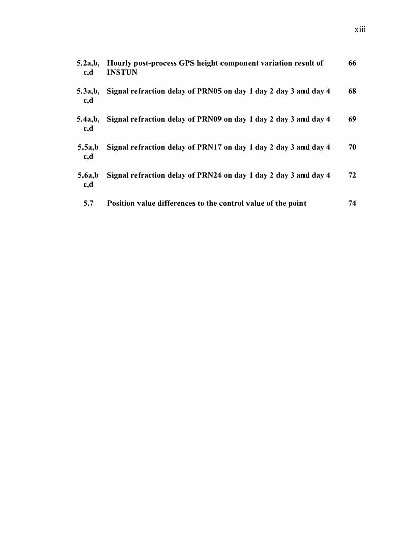
5.2a,b,

c,d Hourly post-process GPS height component variation result of INSTUN

66

5.3a,b, c,d

Signal refraction delay of PRN05 on day 1 day 2 day 3 and day 4 68

5.4a,b, c,d

Signal refraction delay of PRN09 on day 1 day 2 day 3 and day 4 69

5.5a,b c,d

Signal refraction delay of PRN17 on day 1 day 2 day 3 and day 4 70

5.6a,b c,d

Signal refraction delay of PRN24 on day 1 day 2 day 3 and day 4 72

5.7 Position value differences to the control value of the point 74

xiv

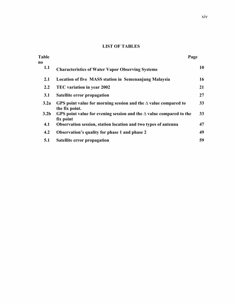
LIST OF TABLES

Table Page no

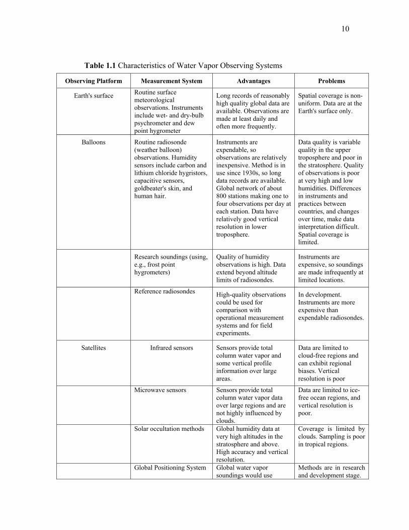
1.1 Characteristics of Water Vapor Observing Systems 10

2.1 Location of five MASS station in Semenanjung Malaysia 16

2.2 TEC variation in year 2002 21

3.1 Satellite error propagation 27

3.2a GPS point value for morning session and the ∆ value compared to the fix point.

33

3.2b GPS point value for evening session and the ∆ value compared to the fix point

33

4.1 Observation session, station location and two types of antenna 47

4.2 Observation’s quality for phase 1 and phase 2 49

5.1 Satellite error propagation 59

1

CHAPTER 1

INTRODUCTION

2

1.0 Overview

The most dense, lowest layer of the earth’s atmosphere is known as the

troposphere. The troposphere is composed of a mixture of several neutral dry

gases, primarily nitrogen and oxygen, and possibly other traces of pollutants. The

air of the troposphere is also contain variable amount of water vapour. The

amount varies depending upon the content of the temperature and pressure of the

air. The highest amount of water vapour can be observed in the Equatorial region

like Malaysia. Knowing that a large amount and strong variation of water vapour

is found in the Equator region, a better understanding of the effect on the Global

Positioning System (GPS) positioning activities is needed. Furthermore, the

information about of water vapour in this region is of special interest for

meteorologists because its behaviour is vital for understanding the global climate,

whereas a short term variation of water vapour is a very useful input to local

weather forecasting.

As the GPS signals propagate from the GPS satellites to the receivers

located on the ground, they are also delayed by the troposphere. The delay can be

represented by a function of satellite elevation and altitude of the GPS receiver,

and is dependent on the atmospheric pressure, temperature and water vapour

pressure. The delay is a wavelength–dependent and thus can not be canceled out

by observing multi-frequency signals. The delay can be evaluated by the

integration of the tropospheric refractivity along the GPS signal path. For

modeling purpose the refractivity is separated into two components, hydrostatic

(dry) and wet components. The hydrostatic component is dependent on the dry air

gasses in the atmosphere and it accounts for approximately 90% of the delay. The

"wet" component depends on the moisture content of the atmosphere and it

accounts for the remaining effect of the delay. Although the dry component has

the larger effect, the errors in the models for the wet component are larger than

3

the errors in the models for the dry because the wet component is more spatially

and temporally varying.

Tropospheric water vapor plays an important role in the global climate

system and is a key variable for short-range numerical weather prediction. Despite

significant progress in remote sensing of wind and temperature, cost-effective

monitoring of atmospheric water vapor is still lacking. Data from the Global

Positioning System (GPS) have recently been suggested to improve this situation.

The tropospheric delay consists of two components. Atmospheric scientists have

shown that GPS determined integrated water vapor from ground-based

observations can significantly improve weather forecasting accuracies (Kuo et al.,

1995). Scientists have reported a worldwide increase in atmospheric water vapor

between the year 1973 to 1985 (see Gaffen et al., 1991). The study was conducted

with radiosonde data only, and similar studies in the future could greatly benefit

from GPS Pressure Water Vapour (GPS PWV) estimates, because of the inherent

homogeneity of the GPS data and their long-term stability. While data from

ground based GPS stations typically provide integrated PWV, data from a GPS

receiver in Low-Earth-Orbit (LEO) can be inverted to measure atmospheric

profiles of refractivity, which in turn can provide tropospheric humidity profiles if

temperature profiles are known. These space-based atmospheric measurements

exploit the fact that a GPS signal that is traveling from a GPS satellite to a LEO is

bent and retarded as it passes through the earth's atmosphere.

1.1 The Current State of Measuring Atmospheric Water Vapor

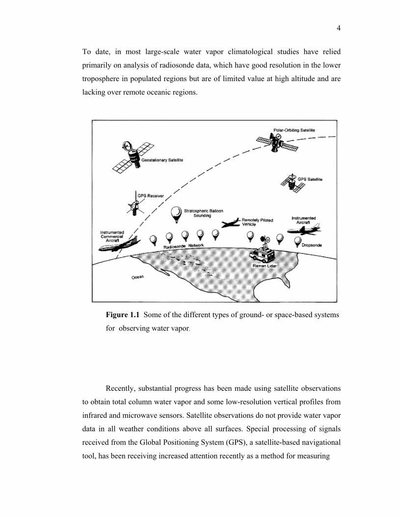
A multitude of systems exist for observing water vapor. Each has different

characteristics and advantages. Figure 1.1 shows some of the different types of

observational systems, while in Table 1.1 compares some of their characteristics.

It is generally agreed that improved knowledge of the role of water vapor in the

climate system hinges largely on closing observational gaps that currently exist.

4

To date, in most large-scale water vapor climatological studies have relied

primarily on analysis of radiosonde data, which have good resolution in the lower

troposphere in populated regions but are of limited value at high altitude and are

lacking over remote oceanic regions.

Figure 1.1 Some of the different types of ground- or space-based systems

for observing water vapor.

Recently, substantial progress has been made using satellite observations

to obtain total column water vapor and some low-resolution vertical profiles from

infrared and microwave sensors. Satellite observations do not provide water vapor

data in all weather conditions above all surfaces. Special processing of signals

received from the Global Positioning System (GPS), a satellite-based navigational

tool, has been receiving increased attention recently as a method for measuring

5

water vapor, as it could give long-term measurements of the total column water

vapor. New water vapor data sets can constructed for several years from a

combination of satellite remote-sensing methods and direct observations to

achieve improved spatial coverage and vertical resolution. Data assimilation

systems, which combine information from observations and output from

atmospheric models, also are being used to augment traditional observations and,

in some instances, to take the place of data where no observations are available.

There are several efforts currently under way to observe, understand, and

model the hydrological cycle and energy fluxes in the atmosphere, on the land

surface, and in the upper ocean. The efforts will investigate variations of the

global hydrological regime and their impact on atmospheric and oceanic

dynamics. Variations in regional hydrological processes and water resources and

their response to change in the environment such as the increase of greenhouse

gases will be examined.

There are questions about how well the current models, both those used in

climate studies and those used in forecasting the daily weather, treat water vapor.

Modeling would be improved by systematic examination of models treatment of

water vapor in light of what is now known of its distributions. Some of the

questions arise because of the lack of good water vapor observations. The likely

benefits of improved water vapor data include better weather forecasts as well as

improved climate models.

Different types of measurements are complementary and useful. The

challenge is how best to merge the available information on water vapor

distribution into an improved description of the time and space variations of water

vapor to enhance climate studies.

High accuracy GPS software estimates the total tropospheric delay in the

zenith direction at regular time intervals. This delay is approximately 250 cm at

sea level and has two components. Wet delay is caused by atmospheric water

6

vapor, and dry or hydrostatic delay by all other atmospheric constituents. The

hydrostatic delay of a zenith GPS signal traveling to an atmospheric depth of

1000 millibars is approximately 230 centimeter. Assuming hydrostatic

equilibrium, this delay can be predicted to better than 1 mm with surface pressure

measurement accuracies of 0.5 millibars. The error introduced by the assumption

of hydrostatic equilibrium depends on winds and topology but is typically of the

order of 0.01%. This corresponds to 0.2 mm in zenith delay. Extreme conditions

may cause an error of several mm.

Wet GPS signal delay ranges from 0 to 40 centimeter in the zenith

direction. The zenith wet delay (ZWD) is highly variable and cannot be accurately

predicted from surface observations. The PWV is the depth of water that would

result if all atmospheric water vapor in a vertical column of air were condensed to

liquid. One centimeter of PWV causes approximately 6.5 centimeter of GPS wet

signal delay.

1.2 Problem Statement

The atmospheric moisture fields that include the water vapour and clouds

remains a difficult problem for improved weather forecasts. In modern weather

prediction, short-term weather forecasts especially in severe weather and

precipitation are essential. The Global Positioning System can be improved all-

weather estimates of the atmospheric refractivity at very low cost compare with

conventional upper-air observing systems.

The applications of GPS has led to a new and potentially significantly

upper-air observing system for meteorological agencies and proposed in the

estimation of integrated precipitable water vapour for the use in objective and

subjective weather forecasting. This technique can be useful for Malaysia.

7

Continuous GPS satellite data incorporated with meteorological parameters can

be use to study the effect of the lower part of the atmosphere.

1.3 Objectives

The main objectives of this project are as follows:-

1. To demonstrate the feasibility of using Global Positioning System (GPS)

and that of ground based meteorological data to provide information for

tropospheric model development.

2. To develop a model and mapping of precipitable water vapours useful for

climate studies.

1.4 Scope of Research

The methodology for the project research involves several parts of

investigations to develop an integrated troposhperic model from ground-based

GPS and meteorological observations for the Malaysian region. The methodology

of this research can be divided into five ( 5 ) phases which are:

Phase 1. Feasibility studies

The first phase that is required is the investigation and studies on existing

techniques in order to provide additional information. This phase consists of

identification of the factors to be considered and the derivation of the parameters

used in the development of the algorithm.

Phase 2. Mathematical formalization and Real time data acquisition

The next phase is the extensive testing with various surface modelling

simulated data will be carried out. Data will be collected from MASS GPS

permanent stations in Malaysia maintained by JUPEM. The data collected by

8

these stations are identified, evaluated and transferred for further processing. The

meteorological data from several sites will be identified and collected.

Phase 3. Data analysis and processing

The meteorological and GPS data are processed for the quality of data.

Then data analysis are carried out. The processing of these data are conducted at

UTM.

Phase 4. Model Development

The modelling and testing of the model will be carried out to determine the

suitable tropospheric model to be used and the capabilities of the model to be

developed.

Phase 5. Verification of Model

Field verification of the tropospheric model which is obtained by integrated

GPS data and that of the ground based meteorological data is required and carried

out at several points. Most of the facilities that are needed in this phase are

available in Universiti Teknologi Malaysia (UTM).

1.5 Contribution

As mentioned earlier, the applications of GPS has led to a new and

potentially significantly upper-air observing system for meteorological agencies

and proposed in the prediction of weather forecasting. This technique can be

useful for Malaysia since the continuous GPS satellite data obtained from Jabatan

Ukur & Pemetaan Malaysia (JUPEM) can be incorporated with meteorological

parameters used to study the effect of the lower part of the atmosphere.

This study can provide benefits to government agencies, scientific

researchers and even public who are interested in current information of weather

9

forecast. Potential mapping system of any low lying areas can be obtained and the

results can show the water level height as indicators for the planning and rescue

purposes. The project is beneficial to researcher at UTM, JUPEM and Malaysian

Meteorological Services since the real time data collected for surveying and

navigation for future references and model developments can be acquired

especially valuable information for short term weather broadcast and improved

weather prediction in Malaysia. The Malaysian public especially the Navigation

community can used this data for navigation purposes.

1.6 Outline Treatment

The integration of GPS and ground based meteorological data in this

research shows the potential of combining the latest technology with some

meteorological data can contribute towards model development. In this chapter

the objectives and the methodology of the research as well as the GPS technology

is introduced. Chapter 2 has been written to describe the research work carried

out in Malaysia by different agencies and the application of atmospheric studies in

Global Navigation Satellite System (GNSS).

In chapter 3, the used of Global Positioning System (GPS) technology in

baseline determination is discussed. The meteorological data is considered to

detect the error sources that resulted from effect of the troposhperic delay. In

chapter 4 the detection of error due to different types of satellite antenna used in

data collection is discussed. In chapter 5 , the test conducted is to detect the effect

of the tropospheric delay in height determination. The meteorological data are

considered in the test carried out. The results in all the studies obtained are

presented at Seminar related to navigation and at International Symposium and

Exhibition on Geoinformation in 2004 and 2005. Through this event the

presentation of the ideas and many opportunities towards the betterment of the

research carried out have been achieved.

10

Table 1.1 Characteristics of Water Vapor Observing Systems

Observing Platform Measurement System Advantages Problems

Earth's surface Routine surface meteorological observations. Instruments include wet- and dry-bulb psychrometer and dew point hygrometer

Long records of reasonably high quality global data are available. Observations are made at least daily and often more frequently.

Spatial coverage is non-uniform. Data are at the Earth's surface only.

Balloons Routine radiosonde (weather balloon) observations. Humidity sensors include carbon and lithium chloride hygristors, capacitive sensors, goldbeater's skin, and human hair.

Instruments are expendable, so observations are relatively inexpensive. Method is in use since 1930s, so long data records are available. Global network of about 800 stations making one to four observations per day at each station. Data have relatively good vertical resolution in lower troposphere.

Data quality is variable quality in the upper troposphere and poor in the stratosphere. Quality of observations is poor at very high and low humidities. Differences in instruments and practices between countries, and changes over time, make data interpretation difficult. Spatial coverage is limited.

Research soundings (using, e.g., frost point hygrometers)

Quality of humidity observations is high. Data extend beyond altitude limits of radiosondes.

Instruments are expensive, so soundings are made infrequently at limited locations.

Reference radiosondes High-quality observations could be used for comparison with operational measurement systems and for field experiments.

In development. Instruments are more expensive than expendable radiosondes.

Satellites Infrared sensors Sensors provide total column water vapor and some vertical profile information over large areas.

Data are limited to cloud-free regions and can exhibit regional biases. Vertical resolution is poor

Microwave sensors Sensors provide total column water vapor data over large regions and are not highly influenced by clouds.

Data are limited to ice-free ocean regions, and vertical resolution is poor.

Solar occultation methods Global humidity data at very high altitudes in the stratosphere and above. High accuracy and vertical resolution.

Coverage is limited by clouds. Sampling is poor in tropical regions.

Global Positioning System Global water vapor soundings would use

Methods are in research and development stage.

11

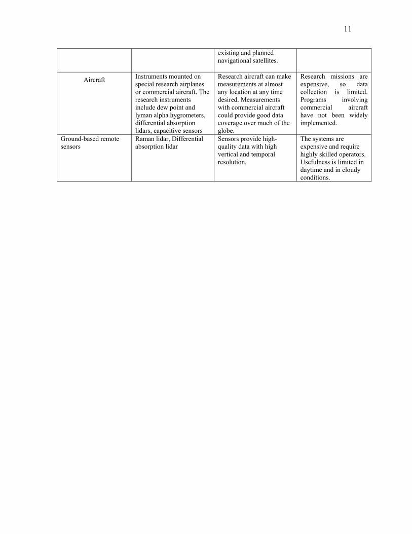
existing and planned navigational satellites.

Aircraft Instruments mounted on special research airplanes or commercial aircraft. The research instruments include dew point and lyman alpha hygrometers, differential absorption lidars, capacitive sensors

Research aircraft can make measurements at almost any location at any time desired. Measurements with commercial aircraft could provide good data coverage over much of the globe.

Research missions are expensive, so data collection is limited. Programs involving commercial aircraft have not been widely implemented.

Ground-based remote sensors

Raman lidar, Differential absorption lidar

Sensors provide high-quality data with high vertical and temporal resolution.

The systems are expensive and require highly skilled operators. Usefulness is limited in daytime and in cloudy conditions.

12

CHAPTER 2 THE APPLICATION OF GNSS FOR ATMOSPHERIC STUDIES IN

MALAYSIA

Md. Nor Kamarudin,1,

Wan Salwa Wan Hassan2,

Zainol Abidin Abdul Rashid 3

1Universiti Teknologi Malaysia, Johor2STRIDE, Ministry of Defence, Jalan Padang Tembak, 50634 Kuala Lumpur, Malaysia 3Universiti Kebangsaan Malaysia, Bangi, Selangor

13

THE APPLICATION OF GNSS FOR ATMOSPHERIC STUDIES IN

MALAYSIA

Abstract

(keywords: Global Positioning System, atmosphere, total electron contents)

Global Positioning System (GPS) satellites provide precise all weather global

navigation information to users equipped with GPS receivers on or near the

earth’s surface. The effects of different error sources on the computed position

have to be removed from the data. In this paper, research work that carried out by

universities and agencies on the atmospheric studies in Malaysia are presented.

Key Researcher:

Md. Nor Kamarudin,1,

Wan Salwa Wan Hassan2,

Zainol Abidin Abdul Rashid 3

14

2.0 Introduction

The ionoshpere is a layer of the atmosphere between 50 km and 1000 km

above the surface of the earth. The ionopshere is made up mostly of O2 and N2.

Solar energy, in the form of ultraviolet light (UV) and x rays, ionize these gases,

allowing electrons to float freely. The Faraday effect introduces phase distortions

in the satellite positioning signals and can lead to large errors, purely due to the

effects of the ionosphere.

Global Positioning System (GPS) satellites provide precise all weather

global navigation information to users equipped with GPS receivers on or near the

earth’s surface. However, irregularities in the electron density of the equatorial

ionosphere, with spatial extent from a few meters to many kilometers, can result

in the performance of GPS receivers to be compromised.

2.1 Total Electron Content (TEC) from GPS

GPS satellites are located about 22,000 km from the earth's surface and

they transmit signals that will be received by GPS receivers on the earth. The

existence of the ionosphere is primarily due to the extreme ultraviolet radiation

and X-rays from the sun. It is a shell of electrons and electrically charged atom

and molecules that surrounds the earth, stretching from the heights of about 50 km

to more than 1000km above the earth's surface. For signal frequency lower than

30 MHz, the ionosphere acts like a reflector. But ultra high frequency radio

waves, like GPS signals, pass through the ionosphere they suffer an extra time

delay as a result of the encounter with the electrons. This time delay is determined

by the density of the electrons, that is characterized by the number of electrons in

a vertical column with a cross-sectional area of one meter along a trans-

ionospheric path to the receiver. This number is called Total Electron Content

(TEC).

15

The TEC which is highly unpredictable depends on many parameter: local

time, season, solar activity geomagnetic activity and latitude (geomagnetic). The

electron density is a function of the amount of incident solar radiation.

TEC is measured in unit of 1016 electron per m2.

1 TECU = 1016 electrons / m2 .

Throughout the day, TEC at a location is dependent on the local time, reaching a

maximum between 12.00 and 16.00. The dispersive nature of the ionosphere

enables measurements of total electron content (TEC) using a dual-frequency

GPS receiver.

One important application for TEC data is in automatic control of aircraft

trajectories, which must be completely accurate. Information on TEC also

provides a valuable tool for investigating global and regional ionospheric

structures. Accurate information on TEC is essential for satellite navigation

systems. The Global Positioning System provides global coverage by definition.

If a suitable network of TEC stations could be established world-wide to use the

GPS signals, TEC data could be available on a near real-time basis. This would

provide near real-time feedback on communications propagation conditions

across the globe.

In addition to instabilities, there are large diurnal and seasonal variations

in the ionosphere in step with solar activity that is almost cyclical every 11 years.

At the equator, such as variations of peaks up during equinoxes in March and

September. These effects are more serious after sunset and during periods of high

solar activity .

16

2.2 Application in Atmospheric Studies

In Malaysia, ionospheric studies is still a relatively new area of research.

The participating from universities and organization to name a few such as

Universiti Teknologi Malaysia, Universiti Kebangsaan Malaysia and STRIDE. In

atmostspheric studies have increased.

2.2.1 Universiti Teknologi Malaysia

The research activities started in 1999 when a group of researchers studied

on the atmospheric refraction effect on GPS positioning. The daily activities of

tracking GPS signals for positioning and mapping purposes have increased the

interest in studying the satellites signal ever since the establishment of Malaysian

Actives Satellite Stations (MASS) in Peninsular Malaysia by Department of

Surveying and Mapping Malaysia (DSMM). Table 2.1 shows the location of

MASS stations used in the research.

GPS signals are obtained from five MASS stations are used to compute

the TEC in the Peninsular region. Data downloaded from GPS receivers are used

to compute the total electron content and the TEC values are plotted for the

region.

Table 2.1 : Location of five MASS station in Semenanjung Malaysia.

Location of Stations Latitude Longitude Height above MSL

Arau

6° 27' 00.57" 100° 16' 47".05 18.12 m

Kuala Lumpur

3° 10' 15.77" 101° 43' 3. "77 112.9 m

Ipoh

4° 35' 18.32" 101° 7' 35. "6 10.8 m

Geting

6° 13' 34.00" 102° 06' 20. "07 13.7 m

Skudai

1° 33' 56.43" 103° 38' 22. "13 87.6 m

17

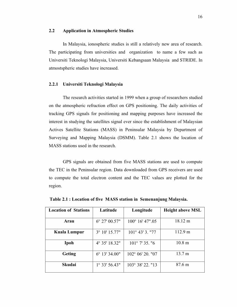
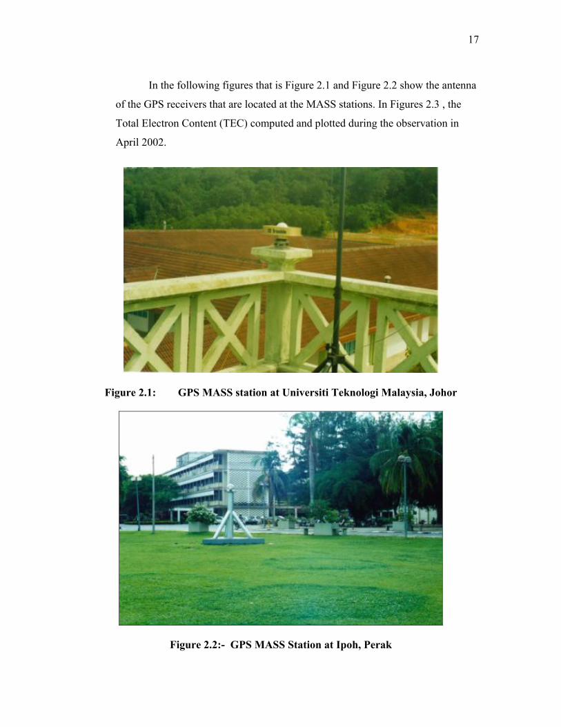
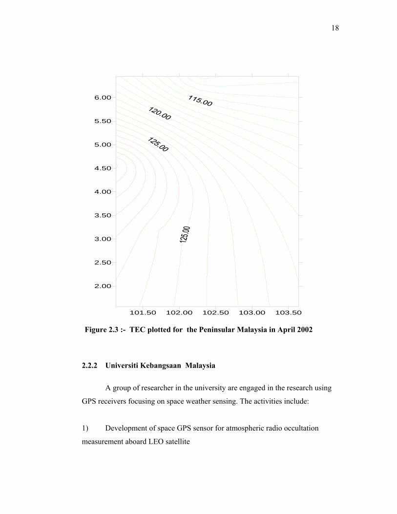
In the following figures that is Figure 2.1 and Figure 2.2 show the antenna

of the GPS receivers that are located at the MASS stations. In Figures 2.3 , the

Total Electron Content (TEC) computed and plotted during the observation in

April 2002.

Figure 2.1: GPS MASS station at Universiti Teknologi Malaysia, Johor

Figure 2.2:- GPS MASS Station at Ipoh, Perak

18

101.50 102.00 102.50 103.00 103.50

2.00

2.50

3.00

3.50

4.00

4.50

5.00

5.50

6.00

Figure 2.3 :- TEC plotted for the Peninsular Malaysia in April 2002

2.2.2 Universiti Kebangsaan Malaysia

A group of researcher in the university are engaged in the research using

GPS receivers focusing on space weather sensing. The activities include:

1) Development of space GPS sensor for atmospheric radio occultation

measurement aboard LEO satellite

19

2) Analysis and Modelling of Polar-Equatorial Ionospheric TEC using GPS

sensing

3) Analysis and Modelling of Polar-Equatorial Ionopsheric Scintillation

using GPS sensing

4) Analysis and Modelling of Polar-Equatrorial Slant Path Water Vapour

using GPS sensing

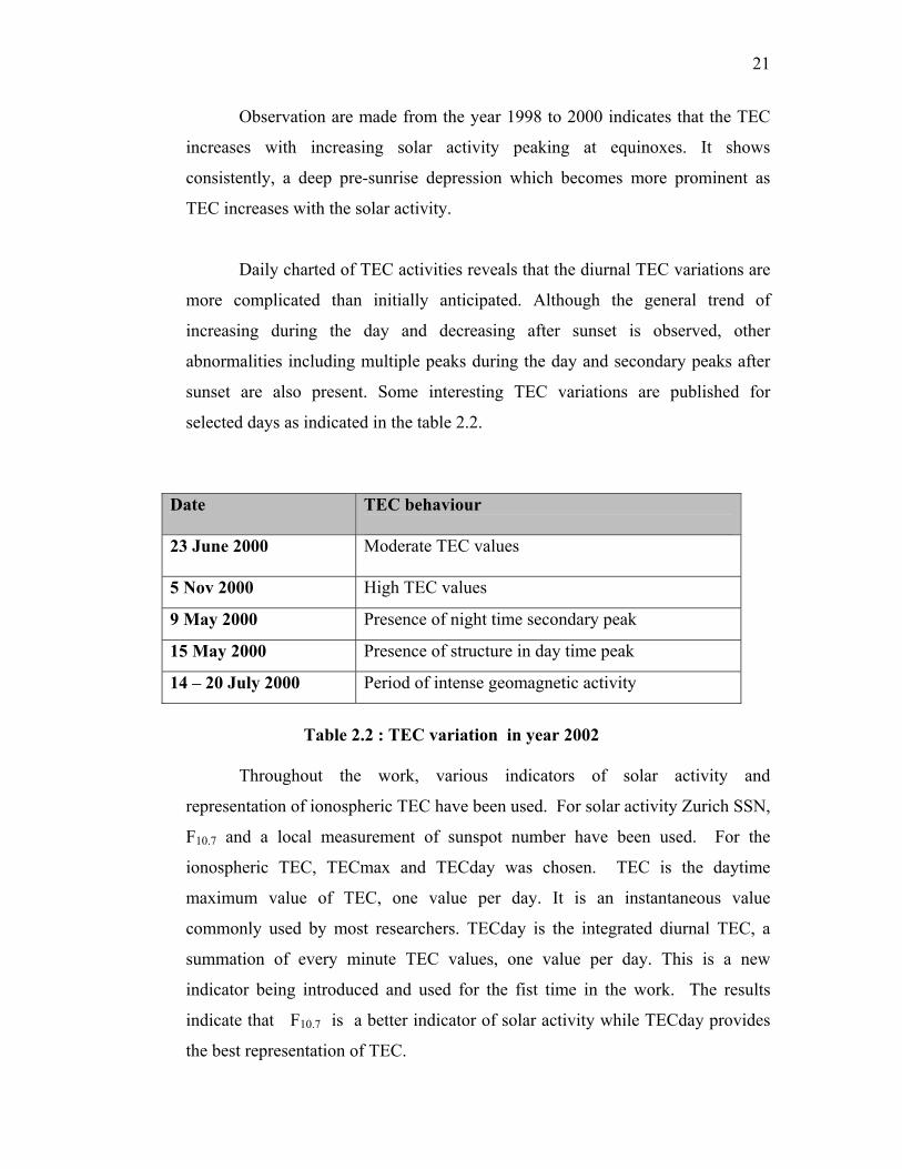
2.2.3 STRIDE Ministry of Defence

In 1998, the Science and Technology Research Institute for Defence

(STRIDE) participated a research through the co-operation with the Defence

Science and Technology Organisation, Australia (DSTO) conducted a long-term

study on the trend of equatorial TEC variations with increasing solar activity

carried out at Marak Parak, Sabah, Malaysia (geographic co-ordinates : 6.31° N,

116.74° E ; geomagnetic lat 1.3° S, dip 3.8° S, declination 0.2° ). Some of the

analysis was carried out jointly with researchers from Universiti Kebangsaan

Malaysia.

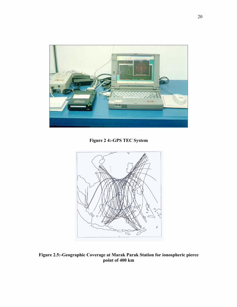
A GPS receiver system, housed in a cabin in Marak Parak, Sabah are used

to study equatorial TEC ionospheric behaviour through continuous reception of

trans-ionospheric GPS signals. The study covers a period near solar maximum

activity in the current solar cycle 23 as it approaches its expected peak towards

the end of 2000

Measurements of ionospheric TEC were done using a NovAtel

MiLLennium GPSCard receiver with NovAtel 503 Survey Antenna and Choke

Ring designed to minimize multipath interference. The dual frequency receiver

has 12 channels permitting simultaneous collection of data from up to 12

satellites. The receiver is placed in a station located on a wide open space and

allows all round clear horizon although on the southwest it is blocked at some

spot by the peak of a mountain at 12°.

20

Figure 2 4:-GPS TEC System

Figure 2.5:-Geographic Coverage at Marak Parak Station for ionospheric pierce point of 400 km

21

Observation are made from the year 1998 to 2000 indicates that the TEC

increases with increasing solar activity peaking at equinoxes. It shows

consistently, a deep pre-sunrise depression which becomes more prominent as

TEC increases with the solar activity.

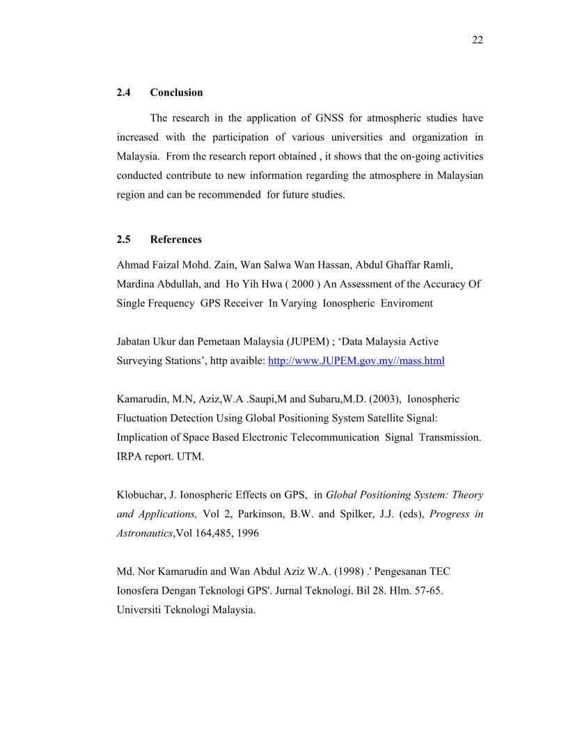
Daily charted of TEC activities reveals that the diurnal TEC variations are

more complicated than initially anticipated. Although the general trend of

increasing during the day and decreasing after sunset is observed, other

abnormalities including multiple peaks during the day and secondary peaks after

sunset are also present. Some interesting TEC variations are published for

selected days as indicated in the table 2.2.

Date TEC behaviour

23 June 2000 Moderate TEC values

5 Nov 2000 High TEC values

9 May 2000 Presence of night time secondary peak

15 May 2000 Presence of structure in day time peak

14 – 20 July 2000 Period of intense geomagnetic activity

Table 2.2 : TEC variation in year 2002

Throughout the work, various indicators of solar activity and

representation of ionospheric TEC have been used. For solar activity Zurich SSN,

F10.7 and a local measurement of sunspot number have been used. For the

ionospheric TEC, TECmax and TECday was chosen. TEC is the daytime

maximum value of TEC, one value per day. It is an instantaneous value

commonly used by most researchers. TECday is the integrated diurnal TEC, a

summation of every minute TEC values, one value per day. This is a new

indicator being introduced and used for the fist time in the work. The results

indicate that F10.7 is a better indicator of solar activity while TECday provides

the best representation of TEC.

22

2.4 Conclusion

The research in the application of GNSS for atmospheric studies have

increased with the participation of various universities and organization in

Malaysia. From the research report obtained , it shows that the on-going activities

conducted contribute to new information regarding the atmosphere in Malaysian

region and can be recommended for future studies.

2.5 References

Ahmad Faizal Mohd. Zain, Wan Salwa Wan Hassan, Abdul Ghaffar Ramli,

Mardina Abdullah, and Ho Yih Hwa ( 2000 ) An Assessment of the Accuracy Of

Single Frequency GPS Receiver In Varying Ionospheric Enviroment

Jabatan Ukur dan Pemetaan Malaysia (JUPEM) ; ‘Data Malaysia Active

Surveying Stations’, http avaible: http://www.JUPEM.gov.my//mass.html

Kamarudin, M.N, Aziz,W.A .Saupi,M and Subaru,M.D. (2003), Ionospheric

Fluctuation Detection Using Global Positioning System Satellite Signal:

Implication of Space Based Electronic Telecommunication Signal Transmission.

IRPA report. UTM.

Klobuchar, J. Ionospheric Effects on GPS, in Global Positioning System: Theory

and Applications, Vol 2, Parkinson, B.W. and Spilker, J.J. (eds), Progress in

Astronautics,Vol 164,485, 1996

Md. Nor Kamarudin and Wan Abdul Aziz W.A. (1998) .' Pengesanan TEC

Ionosfera Dengan Teknologi GPS'. Jurnal Teknologi. Bil 28. Hlm. 57-65.

Universiti Teknologi Malaysia.

23

Thomas R.M.,M.A.Cervera, K.Eftaxiadis, S.L. Manurung, S.Saroso,

Effendy,A.Ghaffar bin Ramli,Wan Salwa Wan Hassan, Hasan Rahman, Mohd

Noh bin Dalimin,K.M.Groves,and Yue-Jin Wang, A Regional GPS Receiver

Network for Monitoring Equatorial Scintillation and Total Electron Content,

Radio Sci.,36,6,1545-1557,2001.

Wang, Y.J. (1995) ‘Monitoring Ionospheric TEC Using GPS’ , IPS Radio and

Space Services Internal Report. Doc. No: IPS YW-95-01.

24

CHAPTER 3

EFFECTS OF TROPOSPHERIC ZENITH DELAY IN SINGLE BASELINE

DETERMINATION

Md.Nor Kamarudin

Mohd.Zahlan Mohd.Zaki

Department of Geomatics Engineering, Faculty of Geoinformation Science and Engineering

Universiti Teknologi Malaysia.

25

EFFECTS OF TROPOSPHERIC ZENITH DELAY IN SINGLE BASELINE

DETERMINATION

ABSTRACT

(Keywords: GPS, Tropospheric zenith delay, MASS station)

In the global positioning system (GPS) surveying for baseline determination, the

principal limiting error source is incorrect modeling of the delay experienced by GPS

signal propagating through the electrically neutral atmosphere, usually referred to as the

tropospheric delay. An experiment was conducted to determine the effect of tropospheric

zenith delay in single baseline determination using Malaysian Active GPS (MASS)

Station and GPS permanent point. The observations involved are the use of on-site

ground meteorological data and satellite zenith angle information from the GPS data. The

result from processed data was compared to the tropospheric delay corrections in GPS

processing software such as Trimble Geomatics Office (TGO) that has certain limitation

due to the default meteorological value. This paper shows that processing with certain

tropospheric delay correction model using synchronizes ground meteorological and GPS

data at the same point can provide better accurate baseline.

Key Researcher:-

Md. Nor Kamarudin Mohd. Zahlan Mohd. Zaki

26

3.0 Introduction

The lower part of the atmosphere, called the troposphere, is electrically

neutral and non-dispersive for frequencies as high as about 15GHz. In the global

positioning system (GPS) surveying, the principal limiting error source is

incorrect modeling of the delay experienced by GPS signal propagating through

the troposphere, usually referred to as the tropospheric delay.

Within this medium, group and phase velocities of the GPS signal on both

L1 and L2 frequencies are equally reduced. The resulting delay is a function of

atmospheric temperature, pressure, and moisture content. Without appropriate

compensation, tropospheric delay will induce pseudorange and carrier- phase

errors that vary from roughly 2 meters for a satellite at zenith to more than 20

meters for a low-elevation- angle satellite (Hay.C and Wong, 2000). This delay

affects mainly the height component of position and constitutes therefore a matter

of concern in space geodesy applications (Mendes and Langley, 1998).

3.1 Background

3.1.1 The atmospheric effects on GPS signals

In this paper, GPS data are used to estimate the zenith tropospheric delay

from measurement of the delay from each GPS satellite in view from a ground

station. Typically four to six GPS satellites are in view at any given time over the

study area.

GPS signals are affected while being transmitted through the ionosphere

and troposphere (the neutral atmosphere). Normally, the global atmospheric

models are use to correct for the atmospheric effect and these models are suitable

27

for most GPS positioning. For high accuracy static and kinematic applications the

global models are, however not sufficiently accurate (Jensen, 2002).

3.1.2 GPS Error Budget

There are several source of error in GPS and the error sources can be

classified into three groups as

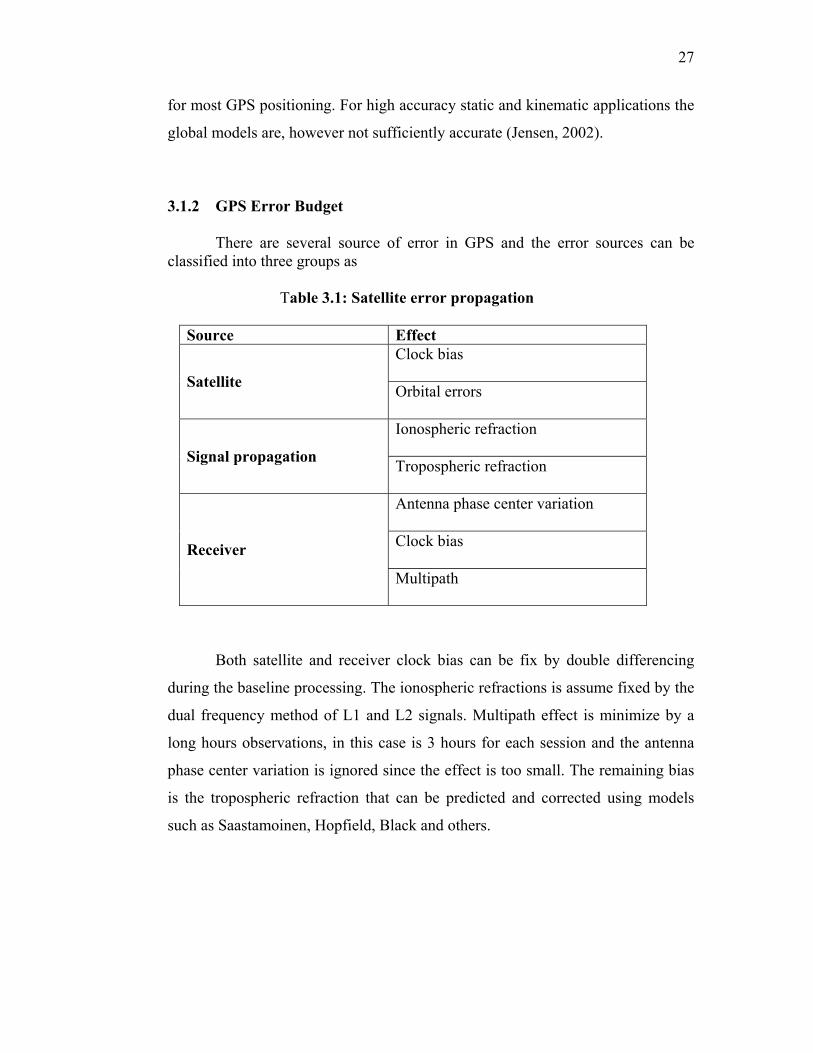
Table 3.1: Satellite error propagation

Source Effect Clock bias Satellite Orbital errors Ionospheric refraction Signal propagation Tropospheric refraction Antenna phase center variation Clock bias Receiver

Multipath

Both satellite and receiver clock bias can be fix by double differencing

during the baseline processing. The ionospheric refractions is assume fixed by the

dual frequency method of L1 and L2 signals. Multipath effect is minimize by a

long hours observations, in this case is 3 hours for each session and the antenna

phase center variation is ignored since the effect is too small. The remaining bias

is the tropospheric refraction that can be predicted and corrected using models

such as Saastamoinen, Hopfield, Black and others.

28

3.1.3 Residual atmospheric effects

Tropospheric layer is the most dynamic among other atmospheric layer

because of the high variation of its water vapor content. This is a major task and

an appropriate model has not yet been found.

Within the tropospheric layer, group and phase velocities of the GPS

signal on both L1 and L2 frequencies are equally reduced. Without appropriate

compensation, tropospheric delay will induce pseudorange and carrier phase

errors that vary from roughly 2 meters for a satellite at zenith to more than 20

meters for a low elevation angle satellite.

3.1.4 The correction methods

The tropospheric delay is composed by two components; one is the dry

part and the other is the wet part. The wet component is more difficult to model

because of the heterogeneous distribution of the water vapor. The dry component

correction is usually carried out using some atmospheric model. The surface

pressure and temperature data are used to compute the dry component delay. In

this experiment, an equation given by Saastamoinen’s (Saastamoinen, 1973) is

use to compute the tropospheric delay including the wet component.

Saastamoinen has refined this model by adding two correction terms, one

being dependent on the height of the observing site and the other on the height

and on the zenith angle. The refine formula is as follows (Hofmann-Wellenhof,

1994):

The equation is given below:

RzBeT

Pz

Trop δ+⎥⎦

⎤⎢⎣

⎡−⎟

⎠⎞

⎜⎝⎛ ++=∆ ²tan05.01255

cos002277.0

where ∆trop is propagation delay in terms of range,

29

z is zenith angle of the satellite,

P is the pressure at the site in milibar,

T is temperature in Kelvin and,

e is the partial pressure of water vapor in milibar.

B, δR is the correction term for height and zenith angle (Hofmann-Wellenhof, 1994).

In the above equation, partial pressure of water vapor is computed from the

relative humidity as a fractional of 1. RH and the temperature, T measured at the

surface. The following equation is used to calculate the partial pressure of water

vapor (Murakami, 1989).

⎥⎦⎤

⎢⎣⎡

−−

×=45.38468415.17exp108.6

TTRHe

RH is relative humidity at site

The pressure P at height above sea level h (in kilometers) is given in terms

of the surface pressure Ps, and temperature Ts as mention by Murakami, 1989 as:

58.7

5.4⎥⎦

⎤⎢⎣

⎡⎟⎠⎞

⎜⎝⎛ −

=Ts

hTsPsP

The dry model is accurate to better than 1 cm (King et al 1985). This is

more than sufficient for the purpose of the orbit determination.The radio signal

delay through the tropospheric is dependent on the total amount of the water

vapor existent along the path. It means that the delay depends on the distribution

of water vapor. The geographical distribution of the clouds is difficult to model.

As a result, a wet component correction using a model is less effective.

Fortunately, the total magnitude of this effect is less than a meter in normal cases.

30

This level of error does not cause a serious problem in the practical application,

especially, when the measured baseline length is short.

3.2 The experiment

3.2.1 The data

Several types of data are use in this experiment such as:

a. MASS station data

b. GPS point

c. Surface meteorological data

d. IGS data product (precise ephemeris)

3.2.2 MASS data

Malaysian Active GPS System (MASS) established Department of Survey

and Mapping Malaysia (DSMM) in providing 24 hours GPS data for GPS users in

Malaysia. This network containing 18 remote stations located strategically to

cover the whole country including the Sabah and Sarawak. The data can be

downloaded by user the day after the actual observations from the website

provided by DSMM. Data from MASS station is use as a control point for the

baseline.

3.2.3 Baseline

Baseline in GPS surveying refers to the position of one receiver relative to

another. When the data from these two receivers is combined, the result is a

baseline comprising a 3-Dimention vector between the two stations. In GPS

processing, a baseline can overcome the effect from the satellite and receiver

clock bias. In theory, this is what we call as double differencing. As the baseline

length and observation periods increase, effects of the troposphere may become

more significant and this leads to tropospheric zenith delay estimation for

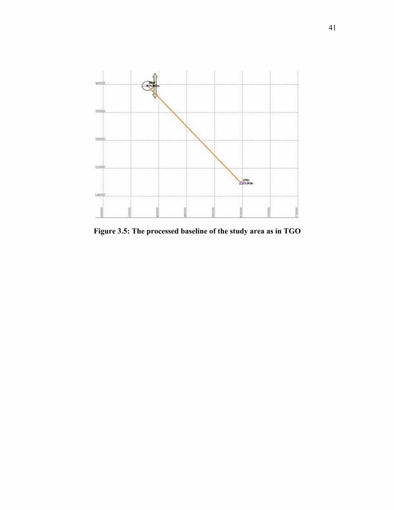
corrections purposes. In this case, the baseline length is 338,855.5255 meter.

31

The instrument used in this experiment is Leica GPS System 500 and

MASS station data derived from UTMJ MASS Station located in Universiti

Teknologi Malaysia.

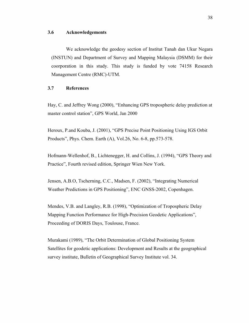
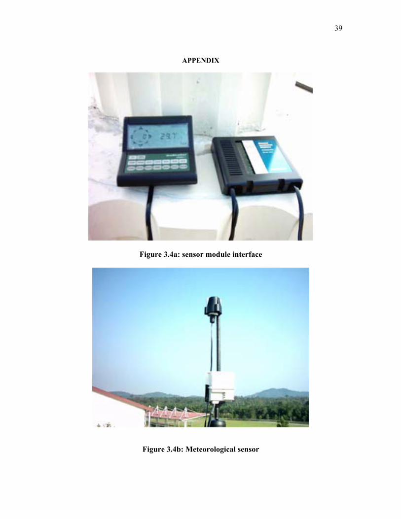
3.2.4 Surface Meteorological Data

A Real time surface meteorological sensor (Davis GroWeather System) is

stationed nearby the GPS receiver to collect the meteorological parameters needed

in the tropospheric model correction algorithm.Surface values of meteorological

data were taken every 10 minutes from 9am to 5pm to see the variations

according to time.

3.2.5 IGS data

IGS precise final orbits is adopted to achieve cm level of accuracy and to

give the exact location of the satellite at any given time. This is to ensure the

value of azimuth and elevation angle of the satellite is corrected before the delay

of each satellite can be determined.

3.3 Processing

Basically, all GPS data need to be processed before it can be used for high

precision purposes. In this experiment, the data was collected using a Leica GPS

receiver but the processing is done using Trimble Geomatic Office (TGO) v1.6.

A baseline processing technique is used to eliminate errors such as clock biases,

orbital errors, ionospheric refraction, cycle slips and multipath which cleaned and

only the tropospheric refraction alone to be fixed.

32

3.3.1 The Model

A refined Saastamoinen model is used in this experiment to estimate the

tropospheric delay in the study area. This has to do with the good reputation of the

model (Saastamoinen) which is widely used for high accuracy GPS positioning

(Jensen, 2002). The accuracy of the Saastamoinen model was estimated to be

about 3cm in zenith (Mendes, 1999).

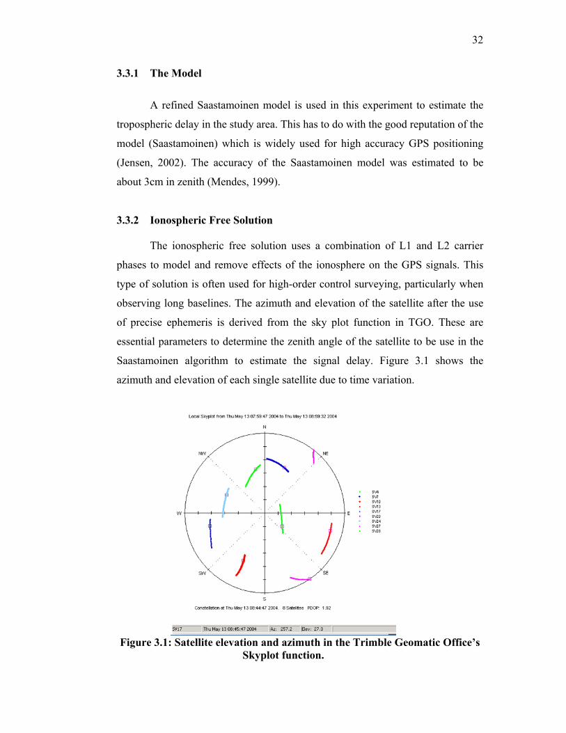
3.3.2 Ionospheric Free Solution

The ionospheric free solution uses a combination of L1 and L2 carrier

phases to model and remove effects of the ionosphere on the GPS signals. This

type of solution is often used for high-order control surveying, particularly when

observing long baselines. The azimuth and elevation of the satellite after the use

of precise ephemeris is derived from the sky plot function in TGO. These are

essential parameters to determine the zenith angle of the satellite to be use in the

Saastamoinen algorithm to estimate the signal delay. Figure 3.1 shows the

azimuth and elevation of each single satellite due to time variation.

Figure 3.1: Satellite elevation and azimuth in the Trimble Geomatic Office’s

Skyplot function.

33

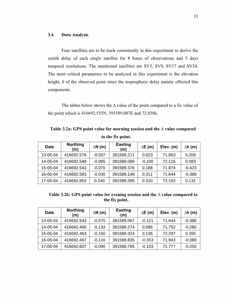
3.4 Data Analysis

Four satellites are to be track consistently in this experiment to derive the

zenith delay of each single satellite for 8 hours of observations and 5 days

temporal resolutions. The mentioned satellites are SV5, SV9, SV17 and SV24.

The most critical parameters to be analyzed in this experiment is the elevation

height, h of the observed point since the tropospheric delay mainly effected this

components.

The tables below shows the ∆ value of the point compared to a fix value of

the point which is 416692.555N, 391589.087E and 72.038h.

Table 3.2a: GPS point value for morning session and the ∆ value compared

to the fix point.

Date Northing (m) ∆N (m) Easting

(m) ∆E (m) Elev. (m) ∆h (m)

13-05-04 416692.576 -0.037 391589.211 0.023 71.853 0.209 14-05-04 416692.548 -0.065 391589.088 -0.100 72.115 0.083 15-05-04 416692.543 -0.070 391589.376 0.188 71.874 -0.423 16-05-04 416692.583 -0.030 391589.146 0.311 71.644 -0.388 17-05-04 416692.853 0.240 391589.395 0.310 72.163 0.131

Table 3.2b: GPS point value for evening session and the ∆ value compared to the fix point.

Date Northing (m) ∆N (m) Easting

(m) ∆E (m) Elev. (m) ∆h (m)

13-05-04 416692.543 -0.070 391589.067 -0.121 71.644 -0.388 14-05-04 416692.480 -0.133 391589.274 0.086 71.752 -0.280 15-05-04 416692.463 -0.150 391589.324 0.136 72.297 0.265 16-05-04 416692.497 -0.116 391588.835 -0.353 71.943 -0.089 17-05-04 416692.607 -0.090 391588.785 -0.103 71.777 -0.255

34

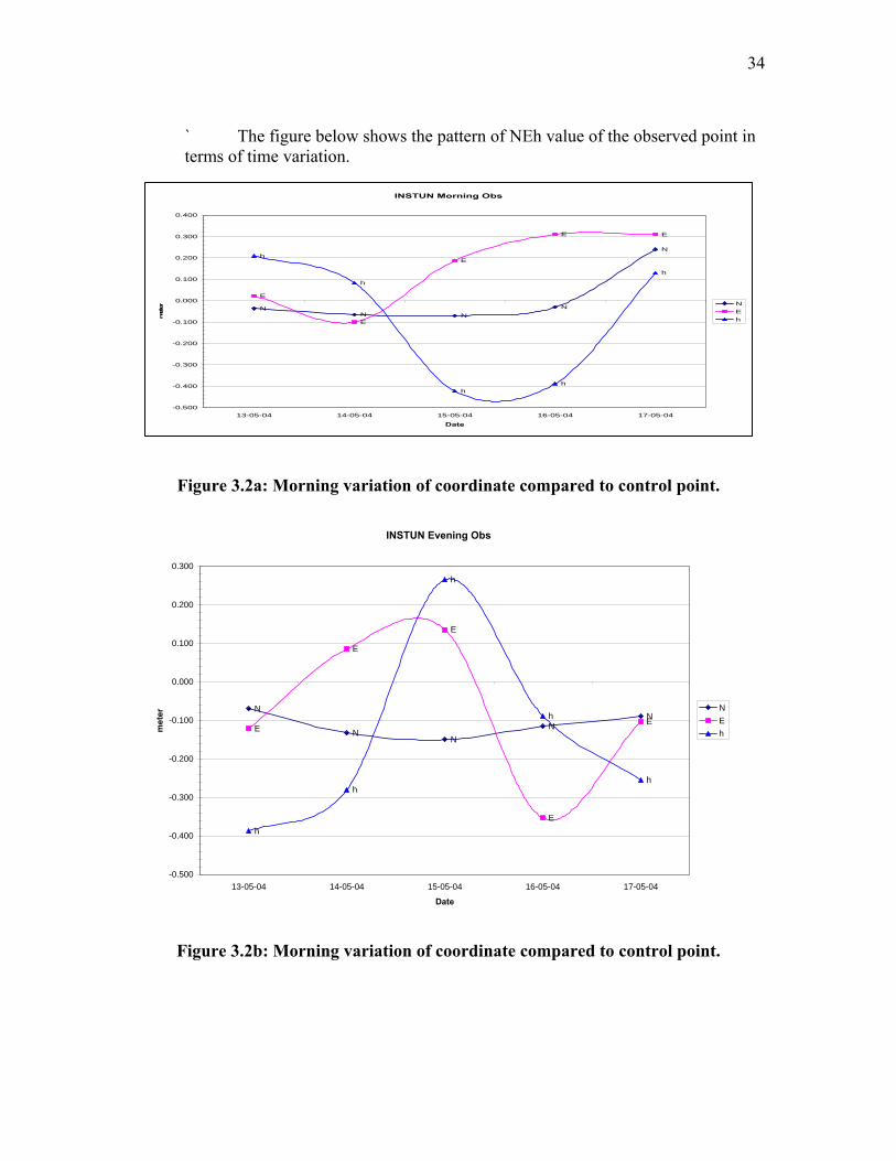
` The figure below shows the pattern of NEh value of the observed point in terms of time variation.

INSTUN Morning Obs

NN N

N

N

E

E

E

E E

h

h

hh

h

-0.500

-0.400

-0.300

-0.200

-0.100

0.000

0.100

0.200

0.300

0.400

13-05-04 14-05-04 15-05-04 16-05-04 17-05-04

Date

meter

NEh

Figure 3.2a: Morning variation of coordinate compared to control point.

INSTUN Evening Obs

N

NN

NN

E

E

E

E

E

h

h

h

h

h

-0.500

-0.400

-0.300

-0.200

-0.100

0.000

0.100

0.200

0.300

13-05-04 14-05-04 15-05-04 16-05-04 17-05-04

Date

met

er

NEh

Figure 3.2b: Morning variation of coordinate compared to control point.

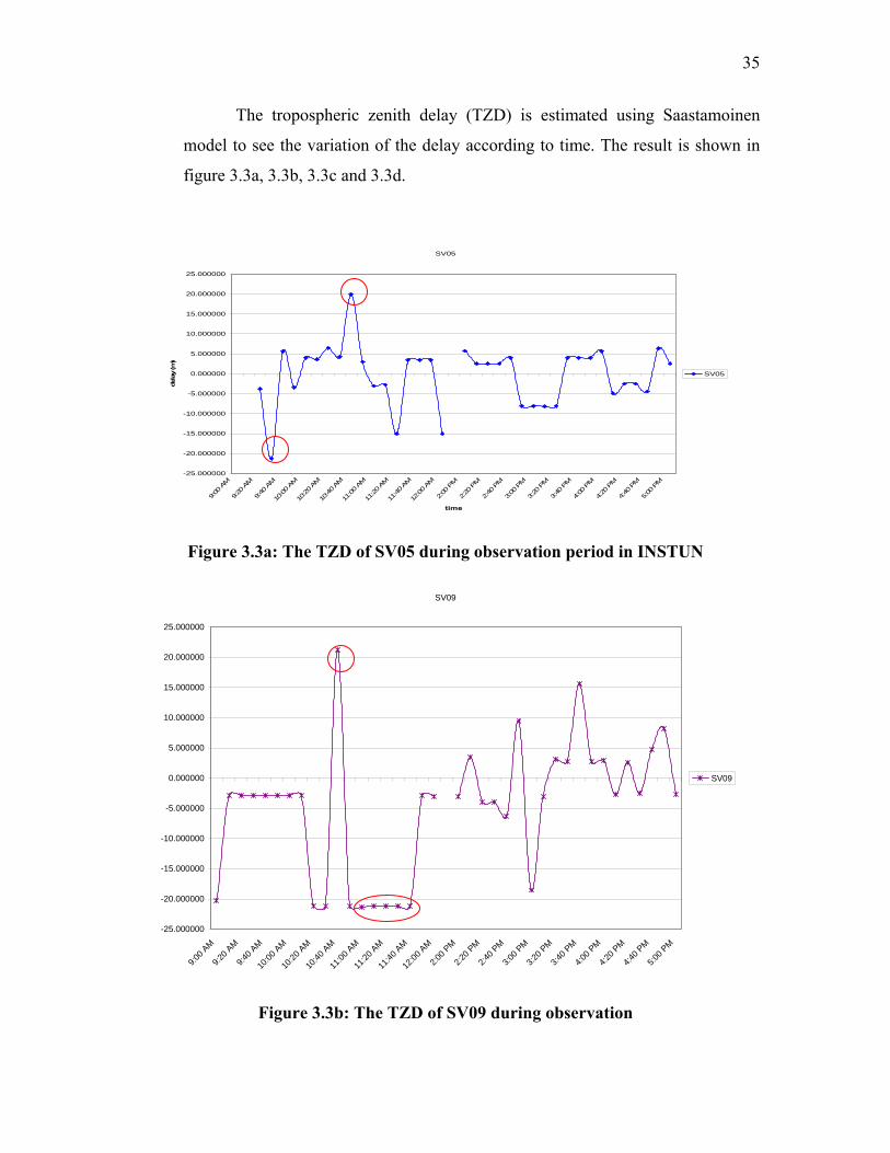
35

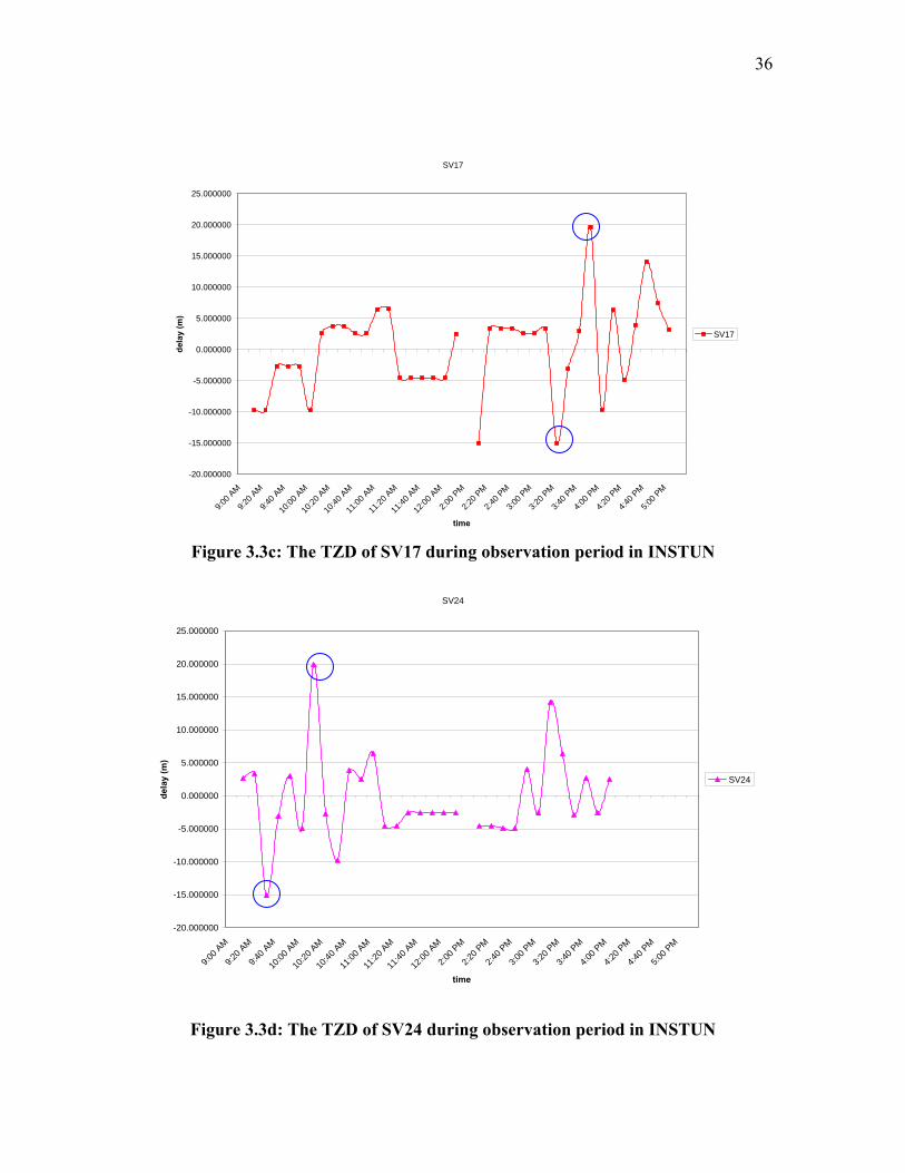
The tropospheric zenith delay (TZD) is estimated using Saastamoinen

model to see the variation of the delay according to time. The result is shown in

figure 3.3a, 3.3b, 3.3c and 3.3d.

SV05

-25.000000

-20.000000

-15.000000

-10.000000

-5.000000

0.000000

5.000000

10.000000

15.000000

20.000000

25.000000

9:00

AM

9:20

AM

9:40

AM

10:00 AM

10:20 AM

10:40 AM

11:00 AM

11:20 AM

11:40 AM

12:00 AM

2:00

PM

2:20

PM

2:40

PM

3:00

PM

3:20

PM

3:40

PM

4:00

PM

4:20

PM

4:40

PM

5:00

PM

time

dela

y (m

)

SV05

Figure 3.3a: The TZD of SV05 during observation period in INSTUN

SV09

-25.000000

-20.000000

-15.000000

-10.000000

-5.000000

0.000000

5.000000

10.000000

15.000000

20.000000

25.000000

9:00 A

M

9:20 A

M

9:40 A

M

10:00

AM

10:20

AM

10:40

AM

11:00

AM

11:20

AM

11:40

AM

12:00

AM

2:00 P

M

2:20 P

M

2:40 P

M

3:00 P

M

3:20 P

M

3:40 P

M

4:00 P

M

4:20 P

M

4:40 P

M

5:00 P

M

SV09

Figure 3.3b: The TZD of SV09 during observation

36

SV17

-20.000000

-15.000000

-10.000000

-5.000000

0.000000

5.000000

10.000000

15.000000

20.000000

25.000000

9:00 A

M

9:20 A

M

9:40 A

M

10:00

AM

10:20

AM

10:40

AM

11:00

AM

11:20

AM

11:40

AM

12:00

AM

2:00 P

M

2:20 P

M

2:40 P

M

3:00 P

M

3:20 P

M

3:40 P

M

4:00 P

M

4:20 P

M

4:40 P

M

5:00 P

M

time

dela

y (m

)

SV17

Figure 3.3c: The TZD of SV17 during observation period in INSTUN

SV24

-20.000000

-15.000000

-10.000000

-5.000000

0.000000

5.000000

10.000000

15.000000

20.000000

25.000000

9:00 A

M

9:20 A

M

9:40 A

M

10:00

AM

10:20

AM

10:40

AM

11:00

AM

11:20

AM

11:40

AM

12:00

AM

2:00 P

M

2:20 P

M

2:40 P

M

3:00 P

M

3:20 P

M

3:40 P

M

4:00 P

M

4:20 P

M

4:40 P

M

5:00 P

M

time

dela

y (m

)

SV24

Figure 3.3d: The TZD of SV24 during observation period in INSTUN

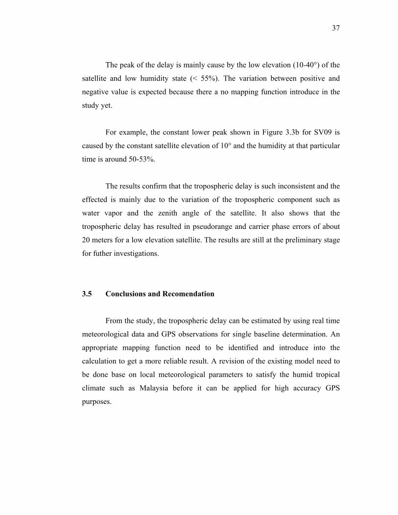
37

The peak of the delay is mainly cause by the low elevation (10-40°) of the

satellite and low humidity state (< 55%). The variation between positive and

negative value is expected because there a no mapping function introduce in the

study yet.

For example, the constant lower peak shown in Figure 3.3b for SV09 is

caused by the constant satellite elevation of 10° and the humidity at that particular

time is around 50-53%.

The results confirm that the tropospheric delay is such inconsistent and the

effected is mainly due to the variation of the tropospheric component such as

water vapor and the zenith angle of the satellite. It also shows that the

tropospheric delay has resulted in pseudorange and carrier phase errors of about

20 meters for a low elevation satellite. The results are still at the preliminary stage

for futher investigations.

3.5 Conclusions and Recomendation

From the study, the tropospheric delay can be estimated by using real time

meteorological data and GPS observations for single baseline determination. An

appropriate mapping function need to be identified and introduce into the

calculation to get a more reliable result. A revision of the existing model need to

be done base on local meteorological parameters to satisfy the humid tropical

climate such as Malaysia before it can be applied for high accuracy GPS

purposes.

38

3.6 Acknowledgements

We acknowledge the geodesy section of Institut Tanah dan Ukur Negara

(INSTUN) and Department of Survey and Mapping Malaysia (DSMM) for their

coorporation in this study. This study is funded by vote 74158 Research

Management Centre (RMC)-UTM.

3.7 References

Hay, C. and Jeffrey Wong (2000), “Enhancing GPS tropospheric delay prediction at

master control station”, GPS World, Jan 2000

Heroux, P.and Kouba, J. (2001), “GPS Precise Point Positioning Using IGS Orbit

Products”, Phys. Chem. Earth (A), Vol.26, No. 6-8, pp.573-578.

Hofmann-Wellenhof, B., Lichtenegger, H. and Collins, J. (1994), “GPS Theory and

Practice”, Fourth revised edition, Springer Wien New York.

Jensen, A.B.O, Tscherning, C.C., Madsen, F. (2002), “Integrating Numerical

Weather Predictions in GPS Positioning”, ENC GNSS-2002, Copenhagen.

Mendes, V.B. and Langley, R.B. (1998), “Optimization of Tropospheric Delay

Mapping Function Performance for High-Precision Geodetic Applications”,

Proceeding of DORIS Days, Toulouse, France.

Murakami (1989), “The Orbit Determination of Global Positioning System

Satellites for geodetic applications: Development and Results at the geographical

survey institute, Bulletin of Geographical Survey Institute vol. 34.

39

APPENDIX

Figure 3.4a: sensor module interface

Figure 3.4b: Meteorological sensor

40

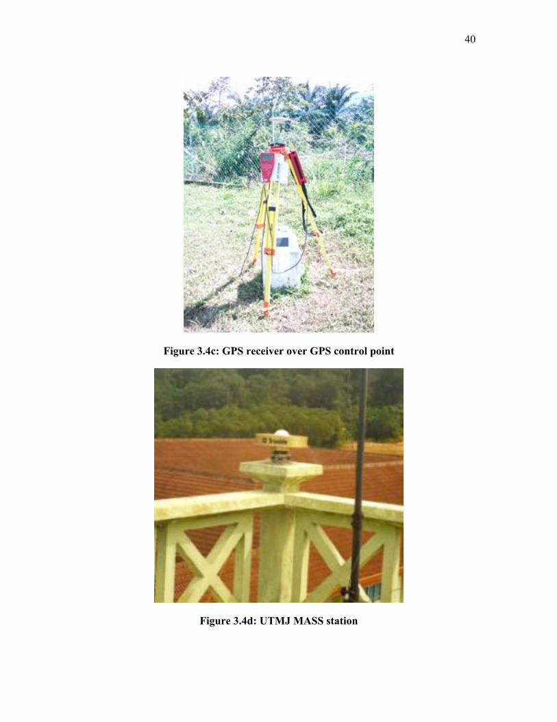
Figure 3.4c: GPS receiver over GPS control point

Figure 3.4d: UTMJ MASS station

41

Figure 3.5: The processed baseline of the study area as in TGO

42

CHAPTER 4

MULTIPATH ERROR DETECTION USING DIFFERENT GPS RECEIVER’S

ANTENNA

Md. Nor Kamarudin

Zulkarnaini Mat Amin

Department of Geomatics Engineering

Faculty of Geoinformation Sciences and Engineering

Universiti Teknologi Malaysia, Skudai, Johor

43

MULTIPATH ERROR DETECTION USING DIFFERENT GPS RECEIVER’S

ANTENNA

ABSTRACT

(Keywords: GPS, multipath error detection, antenna residual.)

The use of satellite based Global Positioning System (GPS) is normal in engineering and

surveying for a wide range of applications as the accuracy capability increases. The GPS

satellites transmit signals that are received by the receivers on the earth’s surface to

determine the position. As long as each satellite’s signal travels along a direct path

straight to the receiver’s antenna, the unit can determine the satellite range quite

accurately. However the ground and other objects easily reflect GPS signals, often

resulting in one or more secondary paths, which are superimposed on the direct-path

signals at the antenna and caused longer propagation time and can significantly distort the

signals waveform’s amplitude and phase. This paper will discussed the detection of the

multipath errors from test carried out using two different types and design of GPS

antenna. The existence of the multipath is analyzed.

Key Researcher:-

Md. Nor Kamarudin

Zulkarnaini Mat Amin

44

4.0 Introduction

Global Positioning System (GPS) is a satellite-based navigation system

that revolutionizes tasks in navigation and surveying. GPS offers several

advantages such as it allows high accuracy in relative positioning, each signal will

pass through the clouds, rains and it can be used day and night regardless weather

condition and also it can be operate 24 hours daily. GPS also gives coordinate

information’s in three dimensional (3D) position of any point.

Every GPS satellite transmits unique navigation signals base on dual-

frequency electromagnetic band which L1 is at 1575.42 MHz and L2 is at

1227.60 MHz. So the frequency of the signal will reflect to the direction when it

hit objects called multipath. Somehow, it still can penetrate the clouds but the

signal will hinder when it pass through heavy fog and thick wet leaves. Basically,

GPS satellite signals consists (Hoffman-Wellenhof et.al., 1997, Leick, 1995 and

Wells et. al., 1987):

i. Dual band frequency – L (L1 and L2)

ii. Modulated frequencies carrier of distance measurement code

iii. Navigation message

All signal components is produced from atomic clock output in high

stabilization. Every satellite is equipped with two cesium atomic clock and two

atomic rubidium clock. These clocks will generate the sinus wave at fo = 10.23

MHz frequency. This frequency is known as basic frequency. Although GPS has

been a great helper in navigation and surveying, but there is situation where the

GPS solution is unreliable and unreachable. The first case happened for bad

satellite’s geometry and GPS multipath error that introduced multiple signals.

The second case happened when the antenna could not receive GPS signals since

it affected from high buildings and other objects in urban areas. This paper will

45

describe the GPS multipath error and several GPS observations have been

conducted using two different antennas; one antenna used to overcome the GPS

multipath (ground plane antenna) problem and another usual antenna supplied by

the manufacturer. Data analysis has been carried out on GPS observation residual

with carrier phase (especially L1 double difference residuals) by calculating the

statistic value and graphically data comparison.

4.1 GPS Multipath Error

Multipath error happens when part of the transmitted signals from satellite

is reflected by the earth surface or any surface that have high power of reflection

before the signals reach to the receiver. This scenario also happen when the

receiver received more secondary path signal from various directions, which

resulted from ireflection from earth surface or any high objects for instance

buildings around the observation station. This interfering signal is neither coded

translated or understandable by GPS receiver.

Magnitude from these multipaths is depends on few factors:

i. Position and types of reflected surface that located near the antenna

ii. The height of antenna from earth surface

iii. GPS wave distance signals

Base on these factors, it clearly shows that received signals from low

altitude satellite have more tendencies to multipath error rather than signals from

higher altitude satellite. Apart from that, range code is more influenced by this

consequences compare to carrier phase. For single reading epoch this error

affected up to 10-20m for pseudo range code (Evans, 1986 and Wells et.al, 1987).

While for carrier phase, this error affected for shorter base line is around 1 cm (for

good satellite’s geometry and longer observation period). Various methods have

46

been conducted to decrease the errors for example by choosing the antenna that

have signals polarization or by filtering signal and applying ground plane antenna

or choke ring. However, the effective method to overcome these errors is by

avoiding the areas or surrounding that may cause multipath problems such as

buildings and other reflected surface.

4.2 Data Collection

The data collection for this study is divided into two phases. In the first

phase, comparison of the observation results at two different areas; one is located

in an open area and the other in an area that has obvious tendencies in causing the

multipath errors. Meanwhile, for the second phase, the data is collected for

evaluating the existing multipath errors in two days consecutively.

In phase 1, the observation has been conducted at station G11 (an open

area), station G12 (area with obvious multipath) and station G13. Station G01

was chosen as reference station since the position is known. For two consecutive

days (25th January 2003 and 26th January 2003) the observation has been carried

out for 2 hours at about the same period of time in order to obtain the same

satellite geometry. Using the same stations, the second phase observation was

continued but an additional station (G13) was observed with a normal antenna to

see the significant change of the multipath error in two days.

In both phases, the data are collected using the receiver of Trimble GPS

4700 with ground plane antenna and Trimble GPS 4800 with normal antenna.

Generally, there are 4 GPS receivers in collecting data simultaneously. The

observation are conducted when GDOP (Geometric Dilution of Precision) value is

less than 3.0 and 15 minutes time interval for 2 hours observation. The GDOP

value indicate the satellite’s geometry with the reference of observation location.

Table 4.1 shows observation session, station location and types of antennas used

47

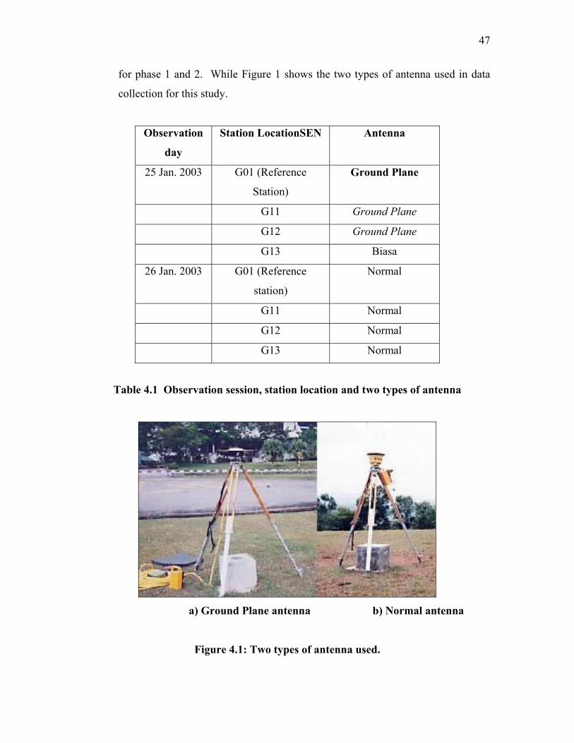
for phase 1 and 2. While Figure 1 shows the two types of antenna used in data

collection for this study.

Observation

day

Station LocationSEN Antenna

25 Jan. 2003 G01 (Reference

Station)

Ground Plane

G11 Ground Plane

G12 Ground Plane

G13 Biasa

26 Jan. 2003 G01 (Reference

station)

Normal

G11 Normal

G12 Normal

G13 Normal

Table 4.1 Observation session, station location and two types of antenna

a) Ground Plane antenna b) Normal antenna

Figure 4.1: Two types of antenna used.

48

4.3 Data Analysis

All observation have been processed with Trimble Geomatic Office

(TGO) software. This software can be used to process baseline and other

additional modules such as for network adjustment and coordinate transformation.

In this study case, the data are processed to the observation accuracy and

observation data residual for every satellite.

The data analysis are carried out in three stages:

i. Compare the quality of the observation due to the surroundings factor

between two different stations.

ii. To identify the residual of every satellite with reference to other existing

antenna in ideal area (zero multipath errors) and area with multipath errors

factors.

iii. Day to day residual analysis for two consecutively days of observation.

4.3.1 Comparing data quality

The analysis is based on the quality of observation from two different

receivers. The parameters involved are ratio value, variance reference and error

in root mean square (RMS) for every observation. The ratio is a relationship

between two variances that was generated from the integer in the processing and

high ratio shows high difference between two choices. Base line processing is

more reliable with high accuracy integer value. Other factors that are relevant

with ratio:

• Higher ratio value is more reliable to every observation.

• Ratio value shows quality point for every quality GPS observation.

• Fixed integer solution produces ratio value.

49

The baseline processing will only solve for ratio value that is more than 1.5.

However, this ratio can possibly varies to higher value or lower value. Reference

variance shows how collected data could fulfill the base line requirement. Base

line processing will predict the error before continue data processing and

comparing the predicted error and actual error obtained during the processing

data. The reading from reference variance should be at 1.000 if the error is

equivalent. The quality for base line solution mostly depends on noise

measurement and satellite’s geometry. RMS uses noise measurement for

observation distance satellite to show solution quality. It also depends on

satellite’s geometry and smaller RMS value.

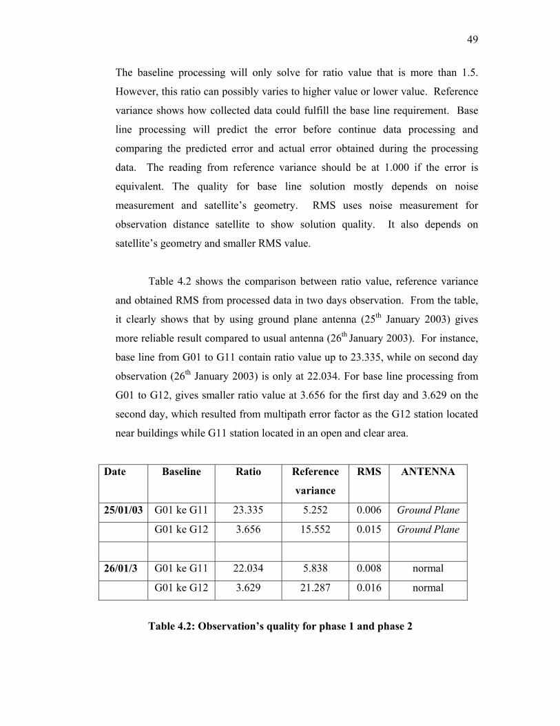
Table 4.2 shows the comparison between ratio value, reference variance

and obtained RMS from processed data in two days observation. From the table,

it clearly shows that by using ground plane antenna (25th January 2003) gives

more reliable result compared to usual antenna (26th January 2003). For instance,

base line from G01 to G11 contain ratio value up to 23.335, while on second day

observation (26th January 2003) is only at 22.034. For base line processing from

G01 to G12, gives smaller ratio value at 3.656 for the first day and 3.629 on the

second day, which resulted from multipath error factor as the G12 station located

near buildings while G11 station located in an open and clear area.

Date Baseline Ratio Reference

variance

RMS ANTENNA

25/01/03 G01 ke G11 23.335 5.252 0.006 Ground Plane

G01 ke G12 3.656 15.552 0.015 Ground Plane

26/01/3 G01 ke G11 22.034 5.838 0.008 normal

G01 ke G12 3.629 21.287 0.016 normal

Table 4.2: Observation’s quality for phase 1 and phase 2

50

4.3.2 Residual Analysis

Apart from ratio factor, reference variance and RMS, the observation

quality can be distinguished through residual observation for every involved

satellite during data collecting process. Residual is a difference value between

observation quantity and calculated value for the quantity, which is carrier phase

value. Residual values have been analyzed to determine the consequences of

multipath error occurred to carrier phase measurement. This study case only used

residual from observation in carrier phase L1. The residual had been plotted

verses time for two different areas.

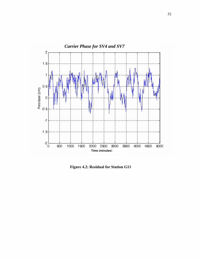
Figure 4.2 shows observation residual value between first day and second

day for integration SV4 and SV7 satellite at observation station G11 (no

interference). On top of that, the residual difference is being calculated from both

SV. Figure 3 shows comparison between two days observation that comprises

areas with multipath error factors, G12 where this area situated near the buildings.

As described in Section 4.2, station surrounding plays an important role to every

GPS observation. In the figure also shows L1 phase value for observation

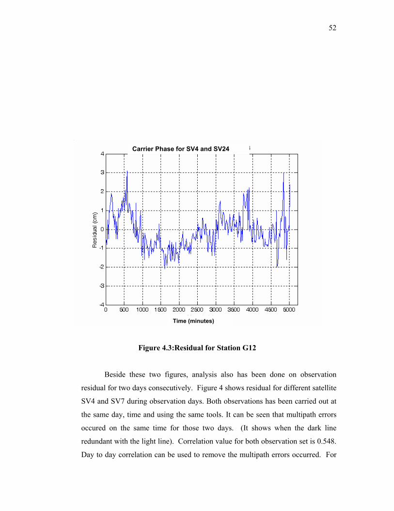
residual for both satellite on the observation day, SV8 and SV24. Standard

deviation value for Figure 4.2 is 0.451 cm, while in Figure 4.3 the value is 0.933

cm.

51

Carrier Phase for SV4 and SV7

)

Figure 4.2:

Time (minutes

Residual for Station G11

52

4

Beside

residual for two

SV4 and SV7 d

the same day, t

occured on the

redundant with

Day to day cor

Carrier Phase for SV4 and SV2

Time (minutes)

Figure 4.3:Residual for Station G12

these two figures, analysis also has been done on observation

days consecutively. Figure 4 shows residual for different satellite

uring observation days. Both observations has been carried out at

ime and using the same tools. It can be seen that multipath errors

same time for those two days. (It shows when the dark line

the light line). Correlation value for both observation set is 0.548.

relation can be used to remove the multipath errors occurred. For

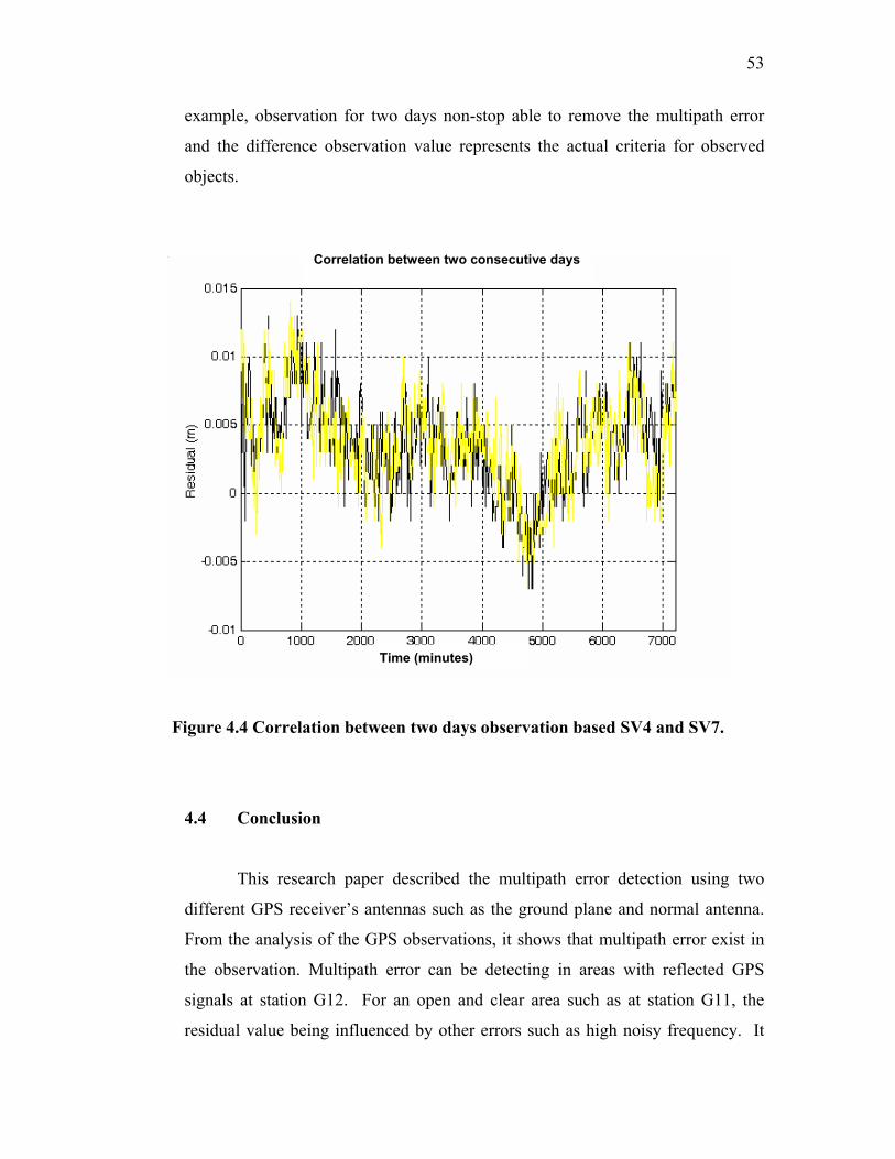
53

example, observation for two days non-stop able to remove the multipath error

and the difference observation value represents the actual criteria for observed

objects.

Correlation between two consecutive days

Time (minutes)

Figure 4.4 Correlation between two days observation based SV4 and SV7.

4.4 Conclusion

This research paper described the multipath error detection using two

different GPS receiver’s antennas such as the ground plane and normal antenna.

From the analysis of the GPS observations, it shows that multipath error exist in

the observation. Multipath error can be detecting in areas with reflected GPS

signals at station G12. For an open and clear area such as at station G11, the

residual value being influenced by other errors such as high noisy frequency. It

54

also shows the ground plane antenna is capable to reduce the multipath errors as

shown in Table 2.

As conclusion, in this study the reliable technique for reducing the

multipath errors was successfully been done by different observation for two days

consecutively. Day to day correlation is useful to apply GPS for observation tasks

such as structural continuous observation. From GPS continuous observation

such as Real Time Kinematics (RTK), the observation output for those two days

has to be differentiated between them in order to obtain the actual object position

in observed area.

4.5 Acknowledgements

Our gratitude goes to En. Jumali Mohd Ismail for his help throughout this

research and Research Management Centre, Universiti Teknologi Malaysia,

81310, Universiti Teknologi Malaysia, Skudai, Johor.

4.6 References

Evans, A.G. (1986), ‘Comparisons of Pseudorange and Biased Doppler Range

Measurements to Demonstrate Signal Multipath Effects’, Proc. of the Fourth

International Geodetic Symposium on Satellite Positioning, Austin, Texas, p. 573-

587.

Geogiadou Y.and Kleusberg A., (1988), ‘On Carrier Signal Multipath Effects in

Relative GPS Positioning’, Manuscripta Geodaetica, vol.13, p. 172-179.

Hoffman-Wellenhof, B, Lichtenegger, B.H. and Collins, J., (1997): ‘Global

Positioning: Theory and Practice’, 4th edition, Springer Verlag.

Leick, A., (1995):’ GPS Satellite Surveying’, John Wiley & Sons, New York, USA.

55

Wells,D. et al, (1987): ‘Guide to GPS Positioning’, Canada GPS Assoc, Fredericton, Canada

56

CHAPTER 5

TROPOSPHERIC DELAY EFFECTS ON RELATIVE GPS HEIGHT DETERMINATION

Md. Nor Kamarudin,

Mohd. Zahlan Mohd. Zaki

Geomatics Engineering Department

Faculty of Geoinformation Science and Engineering

Universiti Teknologi Malaysia

57

TROPOSPHERIC DELAY EFFECTS ON RELATIVE GPS HEIGHT DETERMINATION

ABSTRACT

In the global positioning system (GPS) surveying for point positioning, one of the

principal limiting error source is incorrect modeling of the delay experienced by GPS

signal propagating through the electrically neutral atmosphere, usually referred to as the

tropospheric delay. This paper concentrates on showing the result of an experimental

work that has been conducted by integrating the Malaysian Active GPS Station (MASS)

data and ground meteorological observations to analyze the variation occur to the GPS

height determination due to the tropospheric delay. Four individual satellites are selected

to assist the analysis due to their availability during the observations period. The result of

introducing a Saastamoinen tropospheric model to the data shows a delay variation for up

to 20 meter in pseudorange which causes an error up to 5 meter of height component.

This paper verify that the integration of ground meteorological observations and GPS

lead to a better understanding of the tropospheric delay to the GPS signal and improve

the GPS height accuracy.

Key Researcher:

Md. Nor Kamarudin,

Mohd. Zahlan Mohd. Zaki

58

5.0 Introduction

The troposphere is a part of the earth atmosphere which is situated in its

lower region. It is where all weather occurs, electrically neutral and non-

dispersive for frequencies as high as about 15GHz. In the global positioning

system (GPS) surveying, the principal limiting error source is incorrect modeling

of the delay experienced by GPS signal propagating through the troposphere,

usually referred to as the tropospheric delay.

Within this medium, group and phase velocities of the GPS signal on both

L1 and L2 frequencies are equally reduced. The resulting delay is a function of

atmospheric temperature, pressure, and moisture content represented by relative

humidity. Without appropriate compensation, tropospheric delay will induce

pseudorange and carrier- phase errors that vary from roughly 2 meters for a

satellite at zenith to more than 20 meters for a low-elevation- angle satellite

(Hay.C and Wong, 2000). This delay affects mainly the height component of

position and constitutes therefore a matter of concern in space geodesy

applications (Mendes and Langley, 1998).

5.1 GPS Observations

The constellation of activies GPS satellites consist of 24 satellites. These

satellites are distributed in six orbital planes inclined at 55°, with a nodal

separation of 60°. The orbits are circular with 12 hour period. Each satellite

broadcasts navigation signals on two L band frequencies: 1.57542 GHz (L1) and

1.2276 GHz (L2) carrier phase observations that are used to form ionospheric-free

double differences (Gutman et al., 2003). Sources of initial measurement error

include receiver noise, site-dependant multipath, and antenna phase delays.

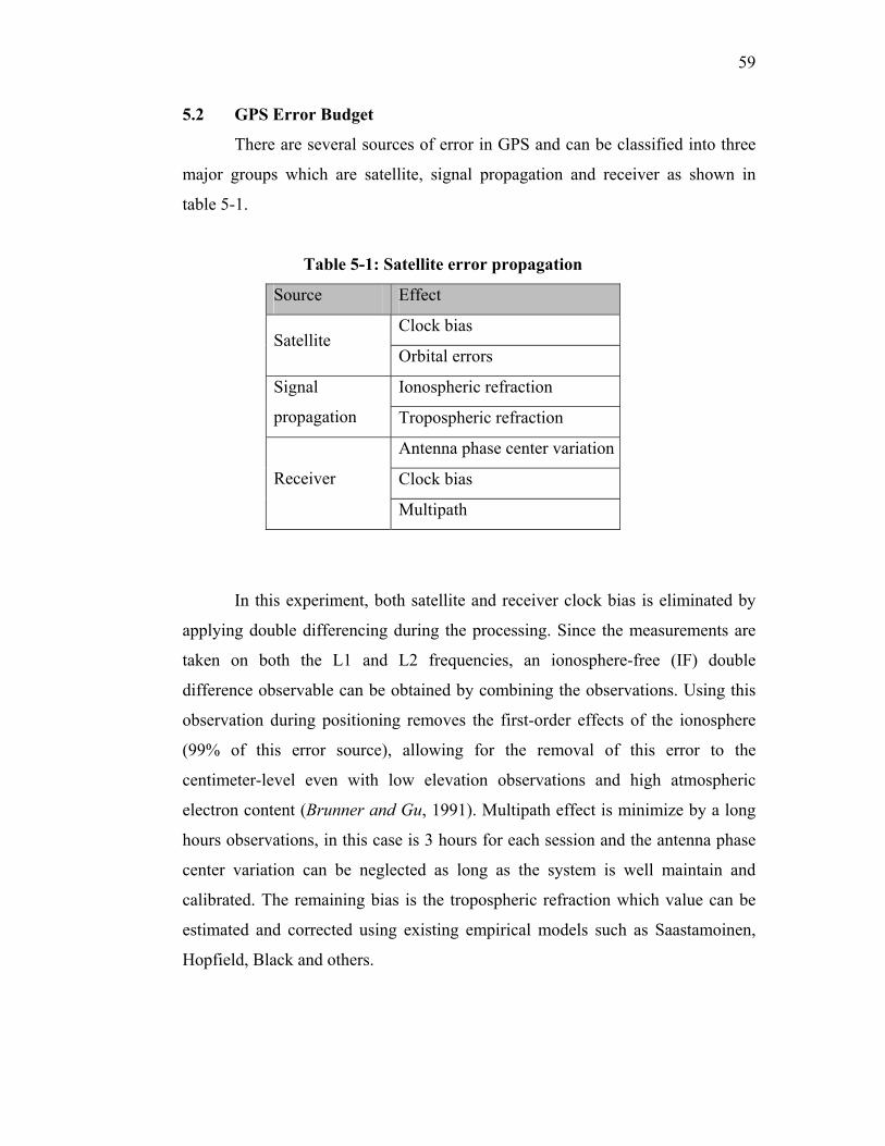
59

5.2 GPS Error Budget

There are several sources of error in GPS and can be classified into three

major groups which are satellite, signal propagation and receiver as shown in

table 5-1.

Table 5-1: Satellite error propagation

Source Effect

Clock bias Satellite

Orbital errors

Ionospheric refraction Signal

propagation Tropospheric refraction

Antenna phase center variation

Clock bias Receiver

Multipath

In this experiment, both satellite and receiver clock bias is eliminated by

applying double differencing during the processing. Since the measurements are

taken on both the L1 and L2 frequencies, an ionosphere-free (IF) double

difference observable can be obtained by combining the observations. Using this

observation during positioning removes the first-order effects of the ionosphere

(99% of this error source), allowing for the removal of this error to the

centimeter-level even with low elevation observations and high atmospheric

electron content (Brunner and Gu, 1991). Multipath effect is minimize by a long

hours observations, in this case is 3 hours for each session and the antenna phase

center variation can be neglected as long as the system is well maintain and

calibrated. The remaining bias is the tropospheric refraction which value can be

estimated and corrected using existing empirical models such as Saastamoinen,

Hopfield, Black and others.

60

5.3 Surface Meteorological Observations

Surface observations are required to parse the tropospheric signal delay

into its wet and dry components. Surface temperature measurements can be used

to estimate the mean temperature of the atmosphere with an error of about 2%. In

general, surface pressure measurements with accuracy of about 0.5 hPa, and

surface temperature measurements with accuracy of about 2 degrees are sufficient

(Saastamoinen, 1972). A Real time surface meteorological sensor (Davis

GroWeatherTM System) is stationed nearby the MASS Station to collect the

meteorological parameters needed in the tropospheric model correction algorithm.

Parameters taken are surface temperature, pressure and relative humidity. These

surface values of meteorological data were taken within a 10 minutes interval

from 9am to 5pm to identify the variations.

5.4 Satellite Orbit Accuracy

IGS precise final orbits are adopt to achieve cm level of accuracy and to

give the exact location of the satellite at any given time. This is to ensure the

value of azimuth and elevation angle of the satellite is corrected before the delay

of each satellite can be determined. Precise orbits are available with about 13 days

latency, and are determined from hundreds of ground tracking stations’

measurements. The accuracy of precise orbits is <5 cm [IGS, 2005]. If the

application permits, most processing is done with precise orbits due to the fact

that it provides very complete ephemeris (if a certain satellite ephemeris is not

available at the time the rapid orbit is available, an effort is made to make it

available in the precise ephemeris) and there is enough time to correct blunders

which may have made their way into other orbital products.

61

5.5 Effects on GPS signals

In this research, GPS data are used to estimate the tropospheric delay from

measurement of the delay from each GPS satellite in view from a ground station.

Typically four to six GPS satellites are in view at any given time over the study

area.

GPS signals are affected while being transmitted through the ionosphere

and troposphere (the neutral atmosphere). Normally, the global atmospheric

models are use to correct for the atmospheric effect and these models are suitable

for most GPS positioning. For high accuracy static and kinematic applications the

global models are, however not sufficiently accurate (Jensen, 2002).

5.6 Residual Tropospheric Effects

Tropospheric layer is the most dynamic among other atmospheric layer

because of the high variation of its water vapor content. This is a major task and

an appropriate model has not yet found.When the satellite signals are transmitted

through the troposphere they are refracted, and the refraction is a function of

meteorological conditions. The refraction causes a signal delay has a size of 2-3

meters in zenith depending on meteorological conditions and the altitude of the

GPS receiver. Within the tropospheric layer, group and phase velocities of the

GPS signal on both L1 and L2 frequencies are equally reduced. Without

appropriate compensation, tropospheric delay will induce pseudorange and carrier

phase errors that vary from roughly 2 meters for a satellite at zenith to more than

20 meters for a low elevation angle satellite (Hay.C and Wong, 2000).

5.7 Delay Estimation

The tropospheric delay is actually composed by two components; one is

the dry part and the other is the wet part. The wet component is more

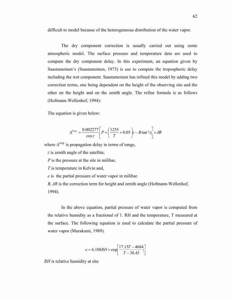
62

difficult to model because of the heterogeneous distribution of the water vapor.

The dry component correction is usually carried out using some

atmospheric model. The surface pressure and temperature data are used to

compute the dry component delay. In this experiment, an equation given by

Saastamoinen’s (Saastamoinen, 1973) is use to compute the tropospheric delay

including the wet component. Saastamoinen has refined this model by adding two

correction terms, one being dependent on the height of the observing site and the

other on the height and on the zenith angle. The refine formula is as follows

(Hofmann-Wellenhof, 1994):

The equation is given below:

RzBeT

Pz

Trop δ+⎥⎦

⎤⎢⎣

⎡−⎟

⎠⎞

⎜⎝⎛ ++=∆ ²tan05.01255

cos002277.0

where ∆trop is propagation delay in terms of range,

z is zenith angle of the satellite,

P is the pressure at the site in milibar,

T is temperature in Kelvin and,

e is the partial pressure of water vapor in milibar.

B, δR is the correction term for height and zenith angle (Hofmann-Wellenhof,

1994).

In the above equation, partial pressure of water vapor is computed from

the relative humidity as a fractional of 1. RH and the temperature, T measured at

the surface. The following equation is used to calculate the partial pressure of

water vapor (Murakami, 1989).

⎥⎦⎤

⎢⎣⎡

−−

×=45.38468415.17exp108.6

TTRHe

RH is relative humidity at site

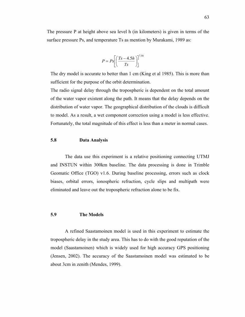
63

The pressure P at height above sea level h (in kilometers) is given in terms of the

surface pressure Ps, and temperature Ts as mention by Murakami, 1989 as:

58.7

5.4⎥⎦

⎤⎢⎣

⎡⎟⎠⎞

⎜⎝⎛ −

=Ts

hTsPsP

The dry model is accurate to better than 1 cm (King et al 1985). This is more than

sufficient for the purpose of the orbit determination.

The radio signal delay through the tropospheric is dependent on the total amount

of the water vapor existent along the path. It means that the delay depends on the

distribution of water vapor. The geographical distribution of the clouds is difficult

to model. As a result, a wet component correction using a model is less effective.

Fortunately, the total magnitude of this effect is less than a meter in normal cases.

5.8 Data Analysis

The data use this experiment is a relative positioning connecting UTMJ

and INSTUN within 300km baseline. The data processing is done in Trimble

Geomatic Office (TGO) v1.6. During baseline processing, errors such as clock

biases, orbital errors, ionospheric refraction, cycle slips and multipath were

eliminated and leave out the tropospheric refraction alone to be fix.

5.9 The Models

A refined Saastamoinen model is used in this experiment to estimate the

tropospheric delay in the study area. This has to do with the good reputation of the

model (Saastamoinen) which is widely used for high accuracy GPS positioning

(Jensen, 2002). The accuracy of the Saastamoinen model was estimated to be

about 3cm in zenith (Mendes, 1999).

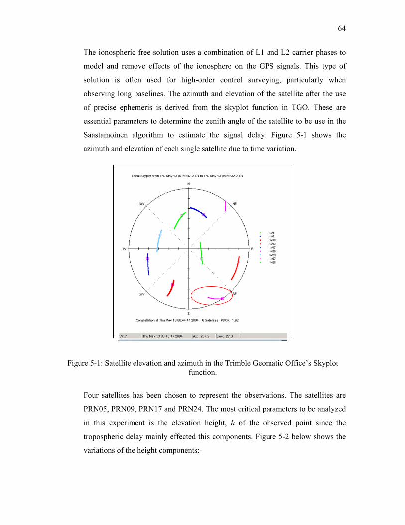
64

The ionospheric free solution uses a combination of L1 and L2 carrier phases to

model and remove effects of the ionosphere on the GPS signals. This type of

solution is often used for high-order control surveying, particularly when

observing long baselines. The azimuth and elevation of the satellite after the use

of precise ephemeris is derived from the skyplot function in TGO. These are

essential parameters to determine the zenith angle of the satellite to be use in the

Saastamoinen algorithm to estimate the signal delay. Figure 5-1 shows the

azimuth and elevation of each single satellite due to time variation.

Figure 5-1: Satellite elevation and azimuth in the Trimble Geomatic Office’s Skyplot function.

Four satellites has been chosen to represent the observations. The satellites are

PRN05, PRN09, PRN17 and PRN24. The most critical parameters to be analyzed

in this experiment is the elevation height, h of the observed point since the

tropospheric delay mainly effected this components. Figure 5-2 below shows the

variations of the height components:-

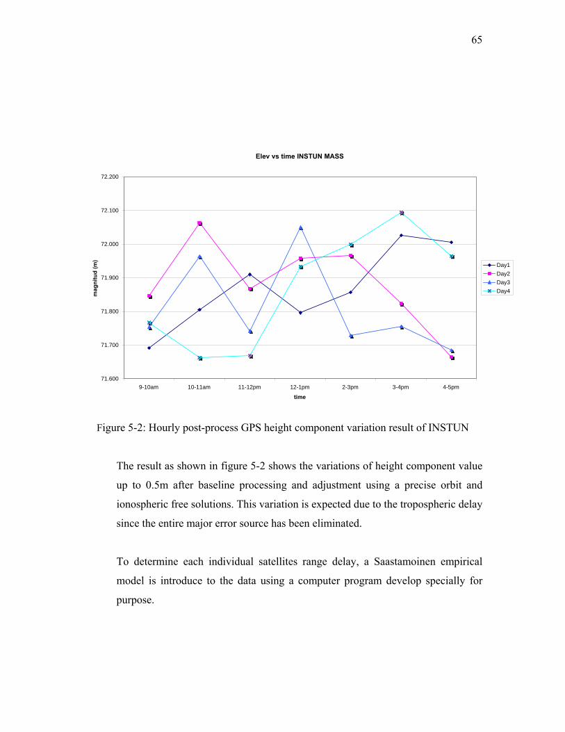
65

Elev vs time INSTUN MASS

71.600

71.700

71.800

71.900

72.000

72.100

72.200

9-10am 10-11am 11-12pm 12-1pm 2-3pm 3-4pm 4-5pm

time

mag

nitu

d (m

)

Day1Day2Day3Day4

Figure 5-2: Hourly post-process GPS height component variation result of INSTUN

The result as shown in figure 5-2 shows the variations of height component value

up to 0.5m after baseline processing and adjustment using a precise orbit and

ionospheric free solutions. This variation is expected due to the tropospheric delay

since the entire major error source has been eliminated.

To determine each individual satellites range delay, a Saastamoinen empirical

model is introduce to the data using a computer program develop specially for

purpose.

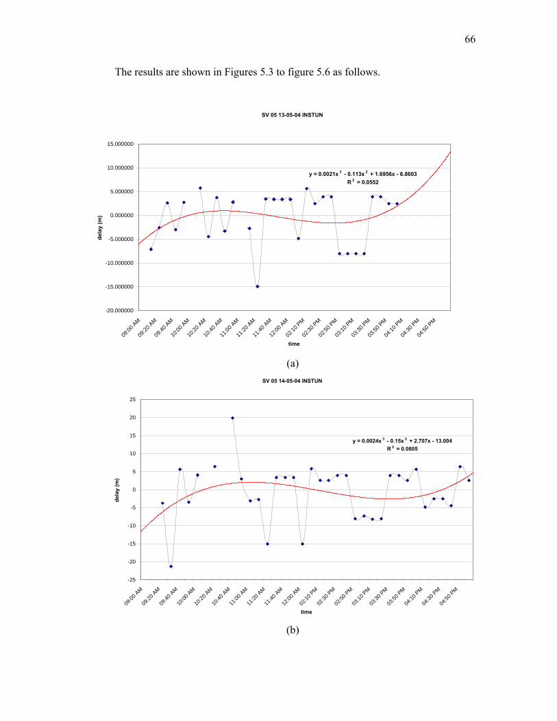
66

The results are shown in Figures 5.3 to figure 5.6 as follows.

SV 05 13-05-04 INSTUN

y = 0.0021x 3 - 0.113x 2 + 1.6956x - 6.8603R 2 = 0.0552

-20.000000

-15.000000

-10.000000

-5.000000

0.000000

5.000000

10.000000

15.000000

09:00

AM

09:20

AM

09:40

AM

10:00

AM

10:20

AM

10:40

AM

11:00

AM

11:20

AM

11:40

AM

12:00

AM

02:10

PM

02:30

PM

02:50

PM

03:10

PM

03:30

PM

03:50

PM

04:10

PM

04:30

PM

04:50

PM

time

dela

y (m

)

(a)

SV 05 14-05-04 INSTUN

y = 0.0024x 3 - 0.15x 2 + 2.707x - 13.004R 2 = 0.0805

-25

-20

-15

-10

-5

0

5

10

15

20

25

09:00

AM

09:20

AM

09:40

AM

10:00

AM

10:20

AM

10:40

AM

11:00

AM

11:20

AM

11:40

AM

12:00

AM

02:10

PM

02:30

PM

02:50

PM

03:10

PM

03:30

PM

03:50

PM

04:10

PM

04:30

PM

04:50

PM

time

dela

y (m

)

(b)

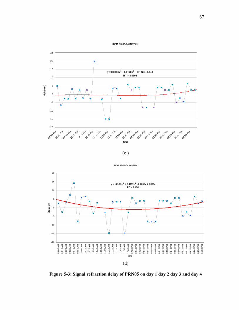
67

SV05 15-05-04 INSTUN

y = 0.0003x 3 - 0.0126x 2 + 0.122x - 0.648R 2 = 0.0156

-20

-15

-10

-5

0

5

10

15

20

25

09:00

AM

09:20

AM

09:40

AM

10:00

AM

10:20

AM

10:40

AM

11:00

AM

11:20

AM

11:40

AM

12:00

AM

02:10

PM

02:30

PM

02:50

PM

03:10

PM

03:30

PM

03:50

PM

04:10

PM

04:30

PM

04:50

PM

time

dela

y (m

)

(c )

SV05 16-05-04 INSTUN

y = -3E-05x 3 + 0.0157x 2 - 0.6056x + 5.0334R 2 = 0.0649

-20

-15

-10

-5

0

5

10

15

20

09:0

0 AM

09:1

0 AM

09:2

0 AM

09:3

0 AM

09:4

0 AM

09:5

0 AM

10:0

0 AM

10:1

0 AM

10:2

0 AM

10:3

0 AM

10:4

0 AM

10:5

0 AM

11:0

0 AM

11:1

0 AM

11:2

0 AM

11:3

0 AM

11:4

0 AM

11:5

0 AM

12:0

0 AM

02:0

0 PM

02:1

0 PM

02:2

0 PM

02:3

0 PM

02:4

0 PM

02:5

0 PM

03:0

0 PM

03:1

0 PM

03:2

0 PM

03:3

0 PM

03:4

0 PM

03:5

0 PM

04:0

0 PM

04:1

0 PM

04:2

0 PM

04:3

0 PM

04:4

0 PM

04:5

0 PM

05:0

0 PM

time

dela

y (m

)

(d)

Figure 5-3: Signal refraction delay of PRN05 on day 1 day 2 day 3 and day 4

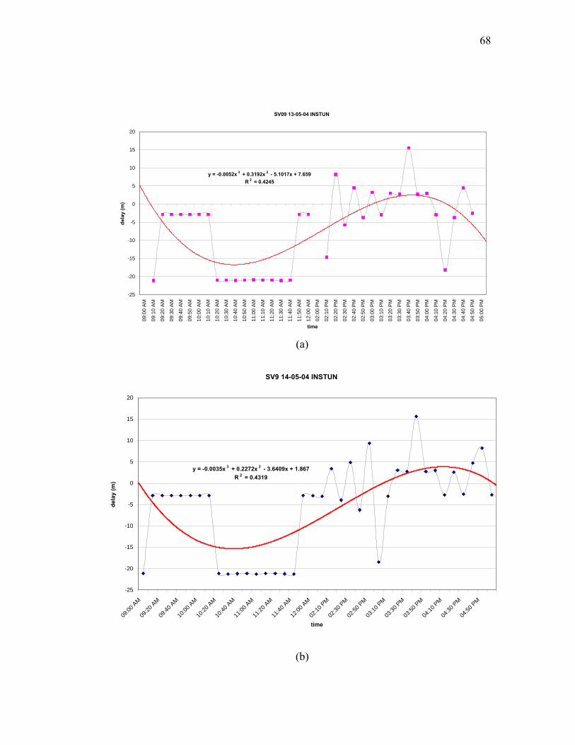
68

SV09 13-05-04 INSTUN

y = -0.0052x 3 + 0.3192x 2 - 5.1017x + 7.659R 2 = 0.4245

-25

-20

-15

-10

-5

0

5

10

15

20

09:0

0 AM

09:1

0 AM

09:2

0 AM

09:3

0 AM

09:4

0 AM

09:5

0 AM

10:0

0 AM

10:1

0 AM

10:2

0 AM

10:3

0 AM

10:4

0 AM

10:5

0 AM

11:0

0 AM

11:1

0 AM

11:2

0 AM

11:3

0 AM

11:4

0 AM

11:5

0 AM

12:0

0 AM

02:0

0 PM

02:1

0 PM

02:2

0 PM

02:3

0 PM

02:4

0 PM

02:5

0 PM

03:0

0 PM

03:1

0 PM

03:2

0 PM

03:3

0 PM

03:4

0 PM

03:5

0 PM

04:0

0 PM

04:1

0 PM

04:2

0 PM

04:3

0 PM

04:4

0 PM

04:5

0 PM

05:0

0 PM

time

dela

y (m

)

(a)

SV9 14-05-04 INSTUN

y = -0.0035x 3 + 0.2272x 2 - 3.6409x + 1.867R 2 = 0.4319

-25

-20

-15

-10

-5

0

5

10

15

20

09:00

AM

09:20

AM

09:40

AM

10:00

AM

10:20

AM

10:40

AM

11:00

AM

11:20

AM

11:40

AM

12:00

AM

02:10

PM

02:30

PM

02:50

PM

03:10

PM

03:30

PM

03:50

PM

04:10

PM

04:30

PM

04:50

PM

time

dela

y (m

)

(b)

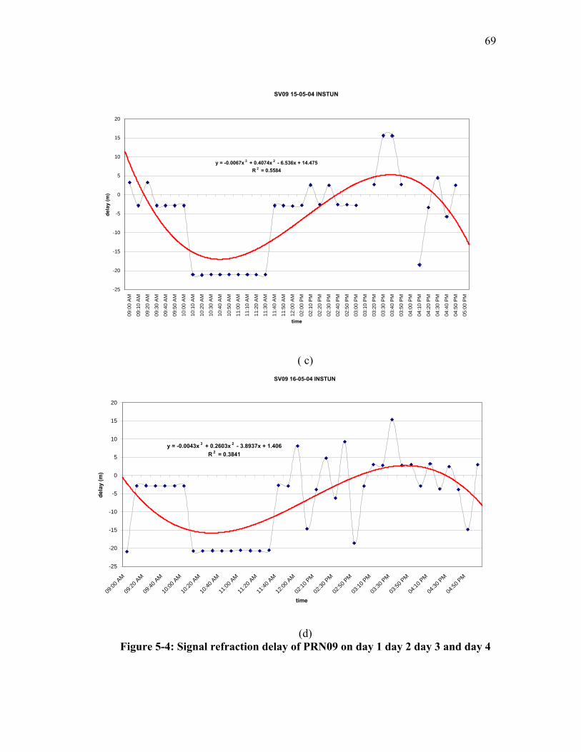
69

SV09 15-05-04 INSTUN

y = -0.0067x 3 + 0.4074x 2 - 6.536x + 14.475R 2 = 0.5584

-25

-20

-15

-10

-5

0

5

10

15

20

09:0

0 AM

09:1

0 AM

09:2

0 AM

09:3

0 AM

09:4

0 AM

09:5

0 AM

10:0

0 AM

10:1

0 AM

10:2

0 AM

10:3

0 AM

10:4

0 AM

10:5

0 AM

11:0

0 AM

11:1

0 AM

11:2

0 AM

11:3

0 AM

11:4

0 AM

11:5

0 AM

12:0

0 AM

02:0

0 PM

02:1

0 PM

02:2

0 PM

02:3

0 PM

02:4

0 PM

02:5

0 PM

03:0

0 PM

03:1

0 PM

03:2

0 PM

03:3

0 PM

03:4

0 PM

03:5

0 PM

04:0

0 PM

04:1

0 PM

04:2

0 PM

04:3

0 PM

04:4

0 PM

04:5

0 PM

05:0

0 PM

time

dela

y (m

)

( c) SV09 16-05-04 INSTUN

y = -0.0043x 3 + 0.2603x 2 - 3.8937x + 1.406R 2 = 0.3841

-25

-20

-15

-10

-5

0

5

10

15

20

09:00

AM

09:20

AM

09:40

AM

10:00

AM

10:20

AM

10:40

AM

11:00

AM

11:20

AM

11:40

AM

12:00

AM

02:10

PM

02:30

PM

02:50

PM

03:10

PM

03:30

PM

03:50

PM

04:10

PM

04:30

PM

04:50

PM

time

dela

y (m

)

(d)

Figure 5-4: Signal refraction delay of PRN09 on day 1 day 2 day 3 and day 4

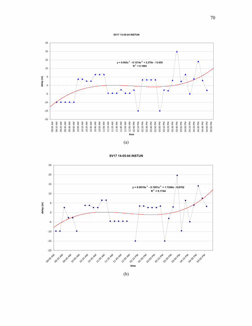
70

SV17 13-05-04 INSTUN

y = 0.002x 3 - 0.1214x 2 + 2.278x - 13.655R 2 = 0.1885

-20

-15

-10

-5

0

5

10

15

20

25

09:0

0 AM

09:1

0 AM

09:2

0 AM

09:3

0 AM

09:4

0 AM

09:5

0 AM

10:0

0 AM

10:1

0 AM

10:2

0 AM

10:3

0 AM

10:4

0 AM

10:5

0 AM

11:0

0 AM

11:1

0 AM

11:2

0 AM

11:3

0 AM

11:4

0 AM

11:5

0 AM

12:0

0 AM

02:0

0 PM

02:1

0 PM

02:2

0 PM

02:3

0 PM

02:4

0 PM

02:5

0 PM

03:0

0 PM

03:1

0 PM

03:2

0 PM

03:3

0 PM

03:4

0 PM

03:5

0 PM

04:0

0 PM

04:1

0 PM

04:2

0 PM

04:3

0 PM

04:4

0 PM

04:5

0 PM

05:0

0 PM

time

dela

y (m

)

(a)

SV17 14-05-04 INSTUN

y = 0.0019x 3 - 0.1051x 2 + 1.7248x - 8.6702R 2 = 0.1744

-20

-15

-10

-5

0

5

10

15

20

25

09:00

AM

09:20

AM

09:40

AM

10:00

AM

10:20

AM

10:40

AM

11:00

AM

11:20

AM

11:40

AM

12:00

AM

02:10

PM

02:30

PM

02:50

PM

03:10

PM

03:30

PM

03:50

PM

04:10

PM

04:30

PM

04:50

PM

time

dela

y (m

)

(b)

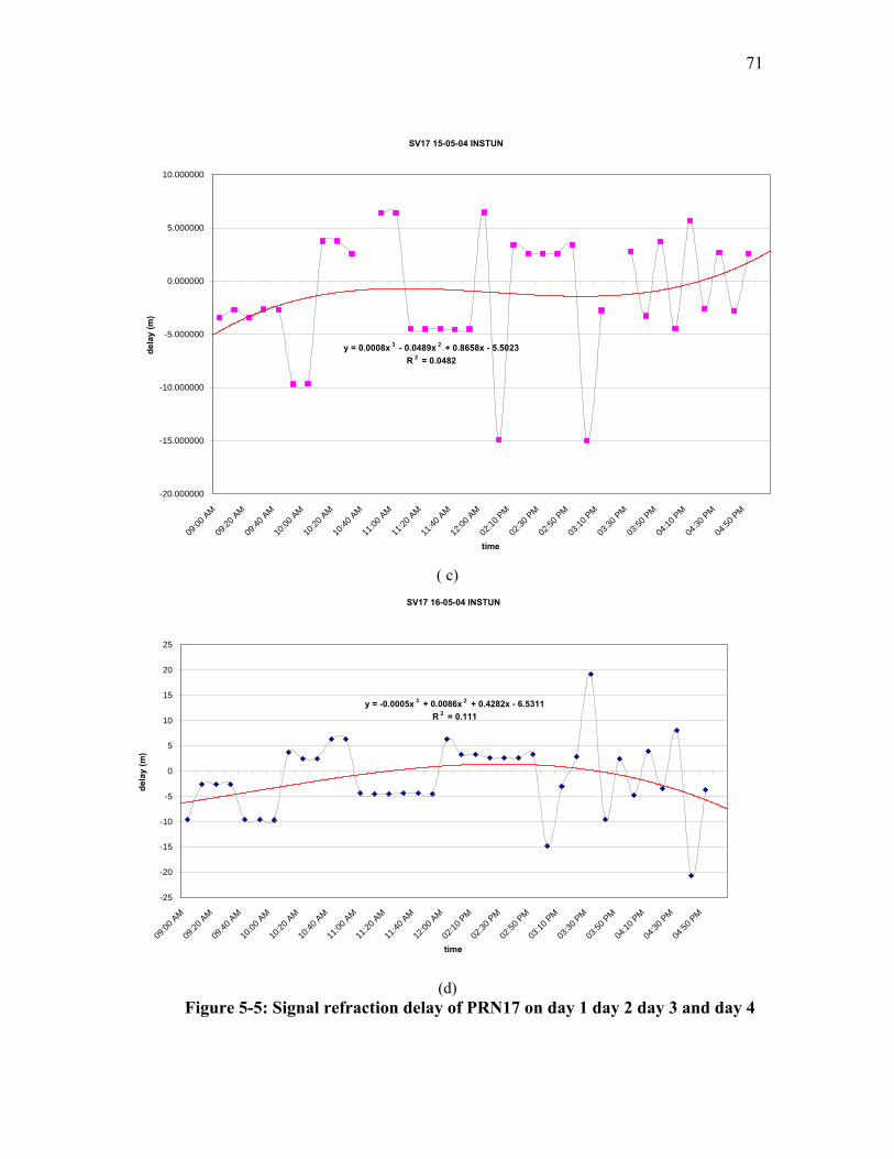
71

SV17 15-05-04 INSTUN

y = 0.0008x 3 - 0.0489x 2 + 0.8658x - 5.5023R 2 = 0.0482

-20.000000

-15.000000

-10.000000

-5.000000

0.000000

5.000000

10.000000

09:00

AM

09:20

AM

09:40

AM

10:00

AM

10:20

AM

10:40

AM

11:00

AM

11:20

AM

11:40

AM

12:00

AM

02:10

PM

02:30

PM

02:50

PM

03:10

PM

03:30

PM

03:50

PM

04:10

PM

04:30

PM

04:50

PM

time

dela

y (m

)

( c)

SV17 16-05-04 INSTUN

y = -0.0005x 3 + 0.0086x 2 + 0.4282x - 6.5311R 2 = 0.111

-25

-20

-15

-10

-5

0

5

10

15

20

25

09:00

AM

09:20

AM

09:40

AM

10:00

AM

10:20

AM

10:40

AM

11:00

AM

11:20

AM

11:40

AM

12:00

AM

02:10

PM

02:30

PM

02:50

PM

03:10

PM

03:30

PM

03:50

PM

04:10

PM

04:30

PM

04:50

PM

time

dela

y (m

)

(d)

Figure 5-5: Signal refraction delay of PRN17 on day 1 day 2 day 3 and day 4

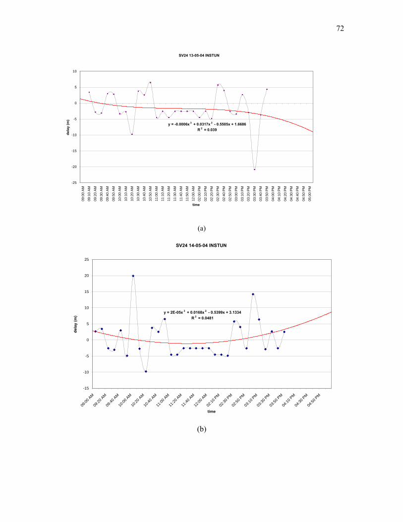
72

SV24 13-05-04 INSTUN

y = -0.0006x 3 + 0.0317x 2 - 0.5505x + 1.6686R 2 = 0.039

-25

-20

-15

-10

-5

0

5

10

09:0

0 AM

09:1

0 AM

09:2

0 AM

09:3

0 AM

09:4

0 AM

09:5

0 AM

10:0

0 AM

10:1

0 AM

10:2

0 AM

10:3

0 AM

10:4

0 AM

10:5

0 AM

11:0

0 AM

11:1

0 AM

11:2

0 AM

11:3

0 AM

11:4

0 AM

11:5

0 AM

12:0

0 AM

02:0

0 PM

02:1

0 PM

02:2

0 PM

02:3

0 PM

02:4

0 PM

02:5

0 PM

03:0

0 PM

03:1

0 PM

03:2

0 PM

03:3

0 PM

03:4

0 PM

03:5

0 PM

04:0

0 PM

04:1

0 PM

04:2

0 PM

04:3

0 PM

04:4

0 PM

04:5

0 PM

05:0

0 PM

time

dela

y (m

)

(a)

SV24 14-05-04 INSTUN

y = 2E-05x 3 + 0.0168x 2 - 0.5399x + 3.1334R 2 = 0.0481

-15

-10

-5

0

5

10

15

20

25

09:00

AM

09:20

AM

09:40

AM

10:00

AM

10:20

AM

10:40

AM

11:00

AM

11:20

AM

11:40

AM

12:00

AM

02:10

PM

02:30

PM

02:50

PM

03:10

PM

03:30

PM

03:50

PM

04:10

PM

04:30

PM

04:50

PM

time

dela

y (m

)

(b)

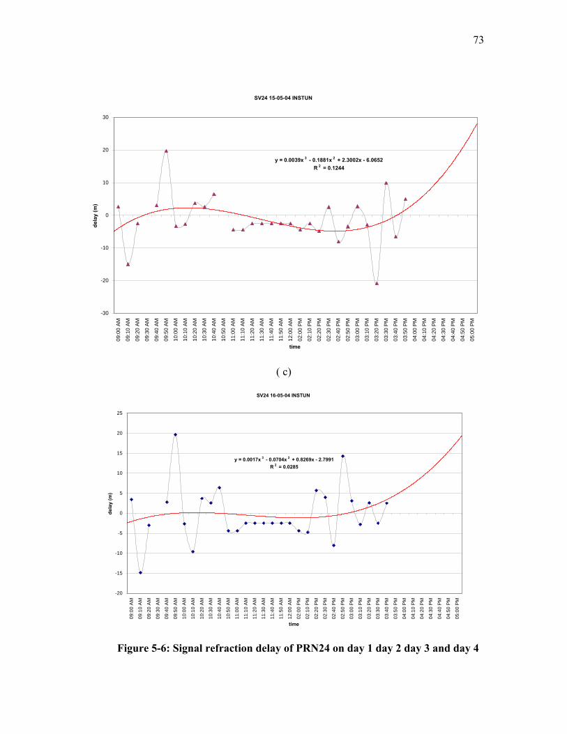
73

SV24 15-05-04 INSTUN

y = 0.0039x 3 - 0.1881x 2 + 2.3002x - 6.0652R 2 = 0.1244

-30

-20

-10

0

10

20

3009

:00

AM

09:1

0 AM

09:2

0 AM

09:3

0 AM

09:4

0 AM

09:5

0 AM

10:0

0 AM

10:1

0 AM

10:2

0 AM

10:3

0 AM

10:4

0 AM

10:5

0 AM

11:0

0 AM

11:1

0 AM

11:2

0 AM

11:3

0 AM

11:4

0 AM

11:5

0 AM

12:0

0 AM

02:0

0 PM

02:1

0 PM

02:2

0 PM

02:3

0 PM

02:4

0 PM

02:5

0 PM

03:0

0 PM

03:1

0 PM

03:2

0 PM

03:3

0 PM

03:4

0 PM

03:5

0 PM

04:0

0 PM

04:1

0 PM

04:2

0 PM

04:3

0 PM

04:4

0 PM

04:5

0 PM

05:0

0 PM

time

dela

y (m

)

( c)

SV24 16-05-04 INSTUN

y = 0.0017x 3 - 0.0704x 2 + 0.8269x - 2.7991R 2 = 0.0285

-20

-15

-10

-5

0

5

10

15

20

25

09:0

0 A

M

09:1

0 A

M

09:2

0 A

M

09:3

0 A

M

09:4

0 A

M

09:5

0 A

M

10:0

0 A

M

10:1

0 A

M

10:2

0 A

M

10:3

0 A

M

10:4

0 A

M

10:5

0 A

M

11:0

0 A

M

11:1

0 A

M

11:2

0 A

M

11:3

0 A

M

11:4

0 A

M

11:5

0 A

M

12:0

0 A

M

02:0

0 P

M

02:1

0 P

M

02:2

0 P

M

02:3

0 P

M

02:4

0 P

M

02:5

0 P

M

03:0

0 P

M

03:1

0 P

M

03:2

0 P

M

03:3

0 P

M

03:4

0 P

M

03:5

0 P

M

04:0

0 P

M

04:1

0 P

M

04:2

0 P

M

04:3

0 P

M

04:4

0 P

M

04:5

0 P

M

05:0

0 P

M

time

dela

y (m

)

Figure 5-6: Signal refraction delay of PRN24 on day 1 day 2 day 3 and day 4

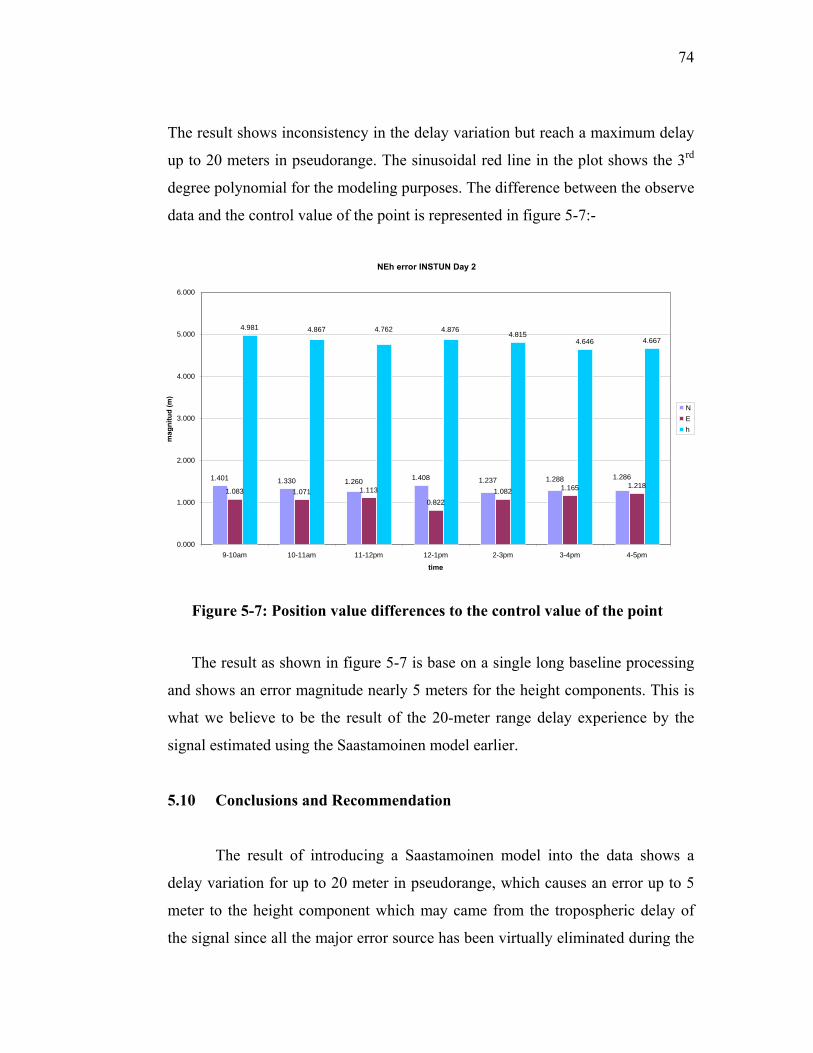
74

The result shows inconsistency in the delay variation but reach a maximum delay

up to 20 meters in pseudorange. The sinusoidal red line in the plot shows the 3rd

degree polynomial for the modeling purposes. The difference between the observe

data and the control value of the point is represented in figure 5-7:-

NEh error INSTUN Day 2

1.401 1.330 1.408

1.083 1.071 1.113

0.8221.082 1.165 1.218

4.9814.815

4.646 4.667

1.2371.260 1.288 1.286

4.8764.867 4.762

0.000

1.000

2.000

3.000

4.000

5.000

6.000

9-10am 10-11am 11-12pm 12-1pm 2-3pm 3-4pm 4-5pm

time

mag

nitu

d (m

)

NEh

Figure 5-7: Position value differences to the control value of the point

The result as shown in figure 5-7 is base on a single long baseline processing

and

5.10 Conclusions and Recommendation

The result of introducing a Saastamoinen model into the data shows a

delay v

shows an error magnitude nearly 5 meters for the height components. This is

what we believe to be the result of the 20-meter range delay experience by the

signal estimated using the Saastamoinen model earlier.

ariation for up to 20 meter in pseudorange, which causes an error up to 5

meter to the height component which may came from the tropospheric delay of

the signal since all the major error source has been virtually eliminated during the

75

processing. This paper verify that the integration of ground meteorological

observations and GPS lead to a better understanding of the tropospheric delay to

the GPS signal and improve the GPS height accuracy.

5.11 ACKNOWLEDGEMENTS

We acknowledge the geodesy section of Institut Tanah dan Ukur Negara

(INSTU

5.12 REFERENCES

Brunner, F.K. and M. Gu, An improved model for the dual frequency ionospheric

Gutman, S.I., S.G. Benjamin, 2001. The Role of Ground-Based GPS

olutions,

Hay, C. and Jeffrey Wong (2000), “Enhancing GPS tropospheric delay prediction at

Heroux, P.and Kouba, J. (2001), “GPS Precise Point Positioning Using IGS Orbit

Hofmann-Wellenhof, B., Lichtenegger, H. and Collins, J. (1994), “GPS Theory and

N), and Department of Survey and Mapping Malaysia (DSMM) for their

coorporation in this study. This study is funded by vote 74158 Research

Management Centre (RMC)-UTM.

correction of GPS observations, Manuscripta Geodaetica, 16, 205, 1991.

Meteorological Observations in Numerical Weather Prediction, GPS S

Volume 4, No. 4, pp. 16-24.

master control station”, GPS World, Jan 2000

Products”, Phys. Chem. Earth (A), Vol.26, No. 6-8, pp.573-578.

Practice”, Fourth revised edition, Springer Wien New York.

76

Jensen, A.B.O, Tscherning, C.C., Madsen, F. (2002), “Integrating Numerical

Weather Predictions in GPS Positioning”, ENC GNSS-2002, Copenhagen.

Mendes, V.B. and Langley, R.B. (1998), “Optimization of Tropospheric Delay

Mapping Function Performance for High-Precision Geodetic Applications”,

Proceeding of DORIS Days, Toulouse, France.

Misra, P. and Enge, P. (2001), “Global Positioning System, Signals, Measurements

and Performance. Ganga-Jamuna Press.

Murakami (1989), “The Orbit Determination of Global Positioning System

Satellites for geodetic applications: Development and Results at the geographical

survey institute, Bulletin of Geographical Survey Institute vol.34.

Saastamoinen, J., (1972). “Introduction to Practical Computation of Astronomical

Refraction”, Bull. Geod., 106, 383-397.

77

CHAPTER 6

SUMMARY AND CONCLUSIONS

78

6.0 Summary

Tropospheric water vapor plays an important role in the global climate

system and is a key variable for short-range numerical weather prediction. Despite

significant progress in remote sensing of wind and temperature, cost-effective

monitoring of atmospheric water vapor is still lacking. Data from the Global

Positioning System (GPS) have recently been suggested to improve this situation.

The highest amount of water vapour can be observed is in the Equatorial

region like Malaysia. Knowing that a large amount and strong variation of water

vapour is found in the Equator region, a better understanding of the effect on the

Global Positioning System (GPS) positioning activities is needed. Furthermore,

the information about of water vapour in this region is of special interest for

meteorologists because the behaviour is vital for understanding the global climate,

whereas a short term variation of water vapour is a very useful input to local

weather forecasting.

As the GPS signals propagate from the GPS satellites to the receivers

located on the ground, they are also delayed by the troposphere. The delay can be

represented by a function of satellite elevation and altitude of the GPS receiver,

and is dependent on the atmospheric pressure, temperature and water vapour

pressure. For modeling purpose the refractivity is separated into two components,

hydrostatic (dry) and wet components. The hydrostatic component is dependent

on the dry air gasses in the atmosphere and it accounts for approximately 90% of

the delay.

The delay can be evaluated by the integration of the tropospheric

refractivity along the GPS signal path, moisture content of the atmosphere and it

accounts for the remaining effect of the delay.

79

High accuracy GPS software estimates the total tropospheric delay in the

zenith direction at regular time intervals. Wet delay is caused by atmospheric

water vapor, and dry or hydrostatic delay by all other atmospheric constituents.

The Global Positioning System can improved all-weather estimates of

the atmospheric refractivity at very low cost compare with conventional upper-air

observing systems. The applications of GPS has led to a new and potentially

significant upper-air observing system for meteorological agencies. It is proposed

in the estimation of integrated precipitable water vapour for the use in objective

and subjective weather forecasting. This technique can be useful for Malaysia.

6.1 Conclusions

Continuous GPS satellite data incorporated with meteorological

parameters can be use to study the effect of the lower part of the atmosphere. The

main objective of this project is to demonstrate the feasibility of using (GPS) and

that of ground based meteorological data to provide information for tropospheric

model development. The development of a model and mapping of precipitable

water vapours useful for climate studies.

In this study an investigation on the existing techniques has been executed

in order to provide additional information. The extensive testing of simulated

data with various surface modeling are carried out and data are collected from

MASS GPS permanent stations in Malaysia maintained by JUPEM. The data

collected by these stations are identified, evaluated and transferred for further

processing. The meteorological data from several sites were identified and

collected and processed for the quality of data. Then data analysis was carried out

using a processing algorithm and was conducted at UTM. The modeling and

testing of the model are carried out to determine the suitable tropospheric model

to be used and the capabilities of the model to be developed. Then the field

verification of the tropospheric model which is obtained by integrated GPS data

and that of the ground based meteorological data several points was tested.

80

The applications of GPS has led to a new and potentially significant

upper-air observing system for meteorological agencies and proposed in the

prediction of weather forecasting. This technique can be useful for Malaysia since

the continuous GPS satellite data obtained from Jabatan Ukur & Pemetaan

Malaysia (JUPEM) can be incorporated with meteorological parameters used to

study the effect of the lower part of the atmosphere. This study can provide

benefits to government agencies, scientific researchers and even public who are

interested in current information of weather forecast. The project is beneficial to

researcher at UTM, JUPEM and Malaysian Meteorological Services since the

real time data collected for surveying and navigation for future references and

model developments can be acquired especially valuable information for short

term weather broadcast and improved weather prediction in Malaysia. The

Malaysian public especially the Navigation community can used this data for

navigation purposes.

The result of introducing a Saastamoinen model into the data shows a

delay variation for up to 20 meter in pseudorange, which causes an error up to 5

meter to the height component which effected from the tropospheric delay of the

signal since all the major error sources have been virtually eliminated during the

processing. The tropospheric delay can be estimated by using real time

meteorological data and GPS observations.

A revision of the existing model has been carried out base on local

meteorological parameters to satisfy the humid tropical climate such as Malaysia

before it can be applied for high accuracy GPS purposes. An appropriate mapping

function need to be identified and introduce into the calculation to get a more

reliable result.

Finally, the study had verified that the integration of ground

meteorological observations and GPS lead to a better understanding of the

tropospheric delay to the GPS signal and improve the GPS height accuracy.

81

REFERENCES

Ahmad Faizal Mohd. Zain, Wan Salwa Wan Hassan, Abdul Ghaffar

Ramli, Mardina Abdullah, and Ho Yih Hwa ( 2000 ) An Assessment

of the Accuracy Of Single Frequency GPS Receiver In Varying

Ionospheric Environment

Bevis M., S. Businger, T.A. Herring, C. Rocken, R.A. Anthes and R.H.

Ware, (1992): GPS Meteorology: Remote Sensing of Atmospheric Water

Vapor using the Global Positioning System, J. Geophys. Res., 97, 15,787-

15,801.

Brunner, F.K. and M. Gu, (1991). An improved model for the dual

frequency ionospheric correction of GPS observations, Manuscripta

Geodaetica, 16, 205, 1991.

Duan, J., M. Bevis, P. Fang, Y. Bock, S.R. Chiswell, S. Businger, C.

Rocken, F. Solheim, R.H. Ware, T. A. Herring and R. W. King,

(1995): Remote sensing atmospheric water vapor using the Global

Positioning System, in review.

Elgered, G., (1993): Tropospheric radio-path delay from ground-based

microwave-radiometry, in Atmospheric Remote Sensing by Microwave

Radiometry, Wiley, ISBN 0-471-62891-3, 215-258.

82

Evans, A.G. (1986), ‘Comparisons of Pseudorange and Biased Doppler

Range Measurements to Demonstrate Signal Multipath Effects’, Proc. of

the Fourth International Geodetic Symposium on Satellite Positioning,

Austin, Texas, p. 573-587.

Gaffen, D.J., T. P. Barnett, and W. P. Elliott, (1991): Space and time

scales of global tropospheric moisture, Journal of Climate, Vol.4, No. 10.

Geogiadou Y.and Kleusberg A., (1988), ‘On Carrier Signal Multipath

Effects in Relative GPS Positioning’, Manuscripta Geodaetica, vol.13, p.

172-179.

Gutman, S.I., S.G. Benjamin, 2001. The Role of Ground-Based GPS

Meteorological Observations in Numerical Weather Prediction, GPS

Solutions, Volume 4, No. 4, pp. 16-24.

Hay, C. and Jeffrey Wong (2000), “Enhancing GPS tropospheric delay

prediction at master control station”, GPS World, Jan 2000

Heroux, P.and Kouba, J. (2001), “GPS Precise Point Positioning Using

IGS Orbit Products”, Phys. Chem. Earth (A), Vol.26, No. 6-8, pp.573-578.

Hoffman-Wellenhof, B, Lichtenegger, B.H. and Collins, J., (1997):

‘Global Positioning: Theory and Practice’, 4th edition, Springer Verlag.

83

Jabatan Ukur dan Pemetaan Malaysia (JUPEM); ‘Data Malaysia

Active Surveying Stations’, http avaible:

http://www.JUPEM.gov.my//mass.html

Jensen, A.B.O, Tscherning, C.C., Madsen, F. (2002), “Integrating

Numerical Weather Predictions in GPS Positioning”, ENC GNSS-2002,

Copenhagen.

Kamarudin, M.N, Aziz,W.A .Saupi,M and Subaru,M.D. (2003),

Ionospheric Fluctuation Detection Using Global Positioning System

Satellite Signal: Implication of Space Based Electronic

Telecommunication Signal Transmission. IRPA report. UTM.

Klobuchar, J (1996). Ionospheric Effects on GPS, in Global Positioning

System: Theory and Applications, Vol 2, Parkinson, B.W. and Spilker, J.J.

(eds), Progress in Astronautics,Vol 164,485,

Kuo, Y.-H., X. Zou andY.-R. Guo (1995)., Variational Assimilation of

precipitable water using a nonhydrostatic Mesoscale Adjoint Model Pat I:

Moisture Retrieval Sensitivity Experiments:

Leick, A., (1995):’ GPS Satellite Surveying’, John Wiley & Sons, New

York, USA

Md. Nor Kamarudin and Wan Abdul Aziz W.A. (1998) .' Pengesanan

TEC Ionosfera Dengan Teknologi GPS'. Jurnal Teknologi. Bil 28. Hlm.

57-65. Universiti Teknologi Malaysia.

84

Mendes, V.B. and Langley, R.B. (1998), “Optimization of Tropospheric

Delay Mapping Function Performance for High-Precision Geodetic

Applications”, Proceeding of DORIS Days, Toulouse, France.

Misra, P. and Enge, P. (2001), “Global Positioning System, Signals,

Measurements and Performance. Ganga-Jamuna Press

Murakami (1989), “The Orbit Determination of Global Positioning

System Satellites for geodetic applications: Development and Results at

the geographical survey institute, Bulletin of Geographical Survey

Institute vol. 34.

Saastamoinen, J., (1972). “Introduction to Practical Computation of

Astronomical Refraction”, Bull. Geod., 106, 383-397.

Thomas R.M., M.A.Cervera, K.Eftaxiadis, S.L. Manurung, S.Saroso,

Effendy, A.Ghaffar bin Ramli,Wan Salwa Wan Hassan, Hasan

Rahman, Mohd Noh bin Dalimin,K.M.Groves,and Yue-Jin Wang,

(2001); A Regional GPS Receiver Network for Monitoring Equatorial

Scintillation and Total Electron Content, Radio Sci.,36,6,1545-1557,.

Wang, Y.J. (1995) ‘Monitoring Ionospheric TEC Using GPS’ , IPS

Radio and Space Services Internal Report. Doc. No: IPS YW-95-01.

Wells,D. et al, (1987): ‘Guide to GPS Positioning’, Canada GPS Assoc,

Fredericton, Canada

85

APPENDIXES

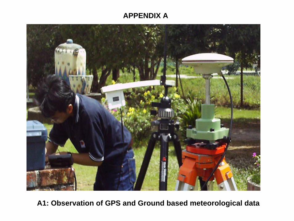
APPENDIX A

A1: Observation of GPS and Ground based meteorological data

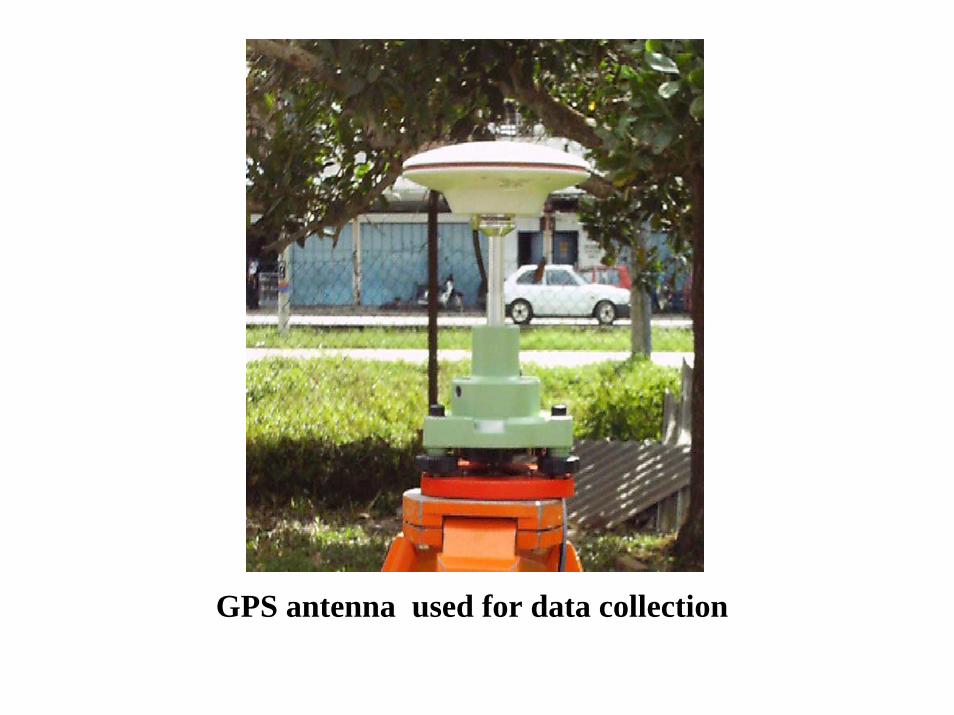
GPS antenna used for data collection

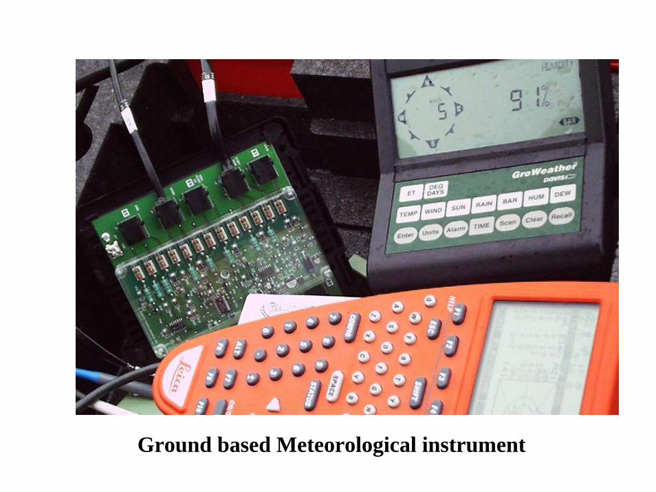
Ground based Meteorological instrument

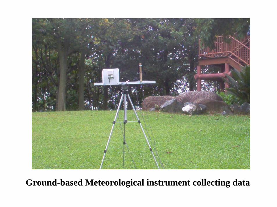
Ground-based Meteorological instrument collecting data

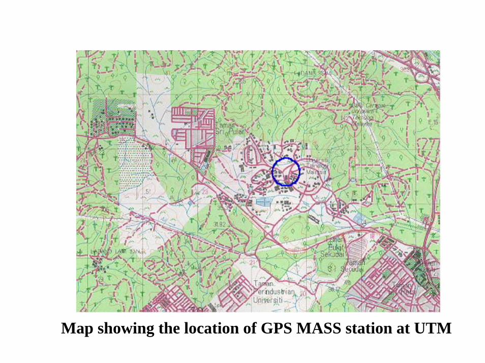
Map showing the location of GPS MASS station at UTM

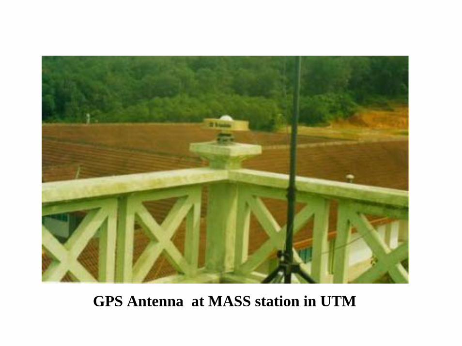
GPS Antenna at MASS station in UTM

APPENDIX B

Acknowledgement:

Special thanks to Meteorological department for the opportunity to visit the KLIA meteorological department in Sepang, Selangor

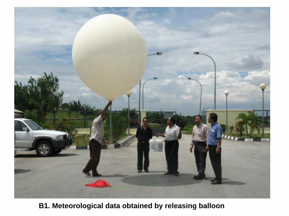
B1. Meteorological data obtained by releasing balloon

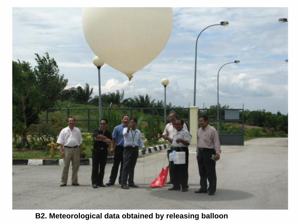
B2. Meteorological data obtained by releasing balloon

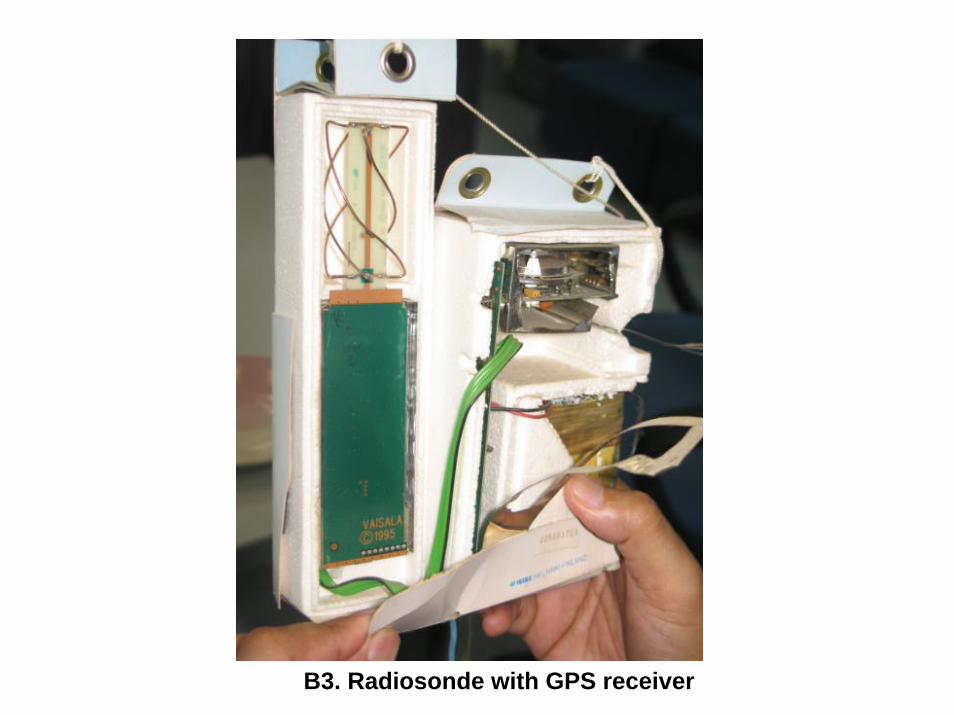
B3. Radiosonde with GPS receiver

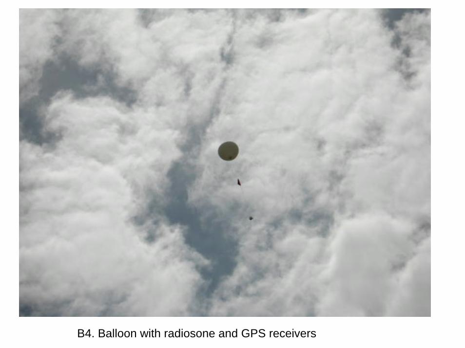
B4. Balloon with radiosone and GPS receivers

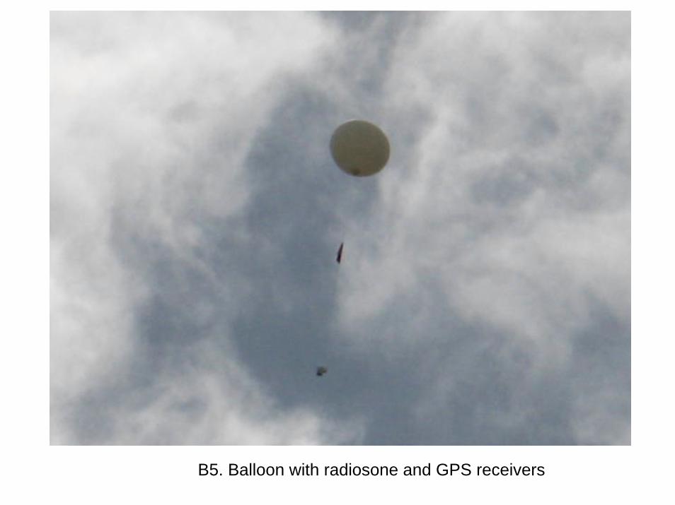
B5. Balloon with radiosone and GPS receivers

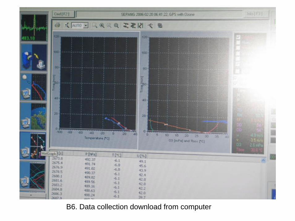
B6. Data collection download from computer