revisiting money demand in malaysia: simple-sum versus ...2)/jeko_52(2)-21.pdf · oleh itu, kajian...

Jurnal Ekonomi Malaysia 52(2) 2018 267 - 278http://dx.doi.org/10.17576/JEM-2018-5202-21

Revisiting Money Demand in Malaysia: Simple-Sum versus Divisia Monetary Aggregates

(Menghayati Semula Permintaan Wang di Malaysia: Penjumlahan Mudah vs Agregat Monetari Divisia)

Chin-Hong PuahUniversiti Malaysia Sarawak

Choi-Meng LeongUCSI University

Abu Mansor ShazaliUniversiti Malaysia Sarawak

Evan LauUniversiti Malaysia Sarawak

AbStrAct

bNM has discarded the use of monetary targeting due to the speeding up of financial reforms as the relationship between money and important macroeconomic indicators in Malaysia has weakened. However, the implementation of the interest rate targeting requires the authorities to alter the policy rate recurrently. Alternatively, the authorities may consider monetary targeting, which provides the ease of control of monetary aggregates, provided that a stable demand for money function can be derived. Nevertheless, financial liberalization has greatly affected the stability of money demand. Thus, this study estimated the demand for money function in Malaysia by considering the effect of the financial development in which a Divisia monetary aggregate has been constructed as an alternative measure of money and a monetization variable has been included in the function. The Johansen and Juselius cointegration test and error correction model are utilized to estimate the demand for money function. The empirical findings indicate that a plausible demand for money function is derived using Divisia M2. Furthermore, monetization appears as an important variable that contributes to a stable money demand. The presence of a stable Divisia M2 money demand has reassured the usefulness of monetary aggregate as the indicator for monetary policy purposes. Monetary targeting provides alternative policy target choice for the conduct of monetary policy. Divisia monetary aggregates can also serve as the alternative money measurement apart from the conventional money supply.

Keywords: Divisia money; financial reform; money demand

AbStrAk

Pembaharuan kewangan yang pesat di Malaysia telah melemahkan hubungan antara wang dengan indikator makroekonomi yang penting dan menyebabkan sasaran monetari telah digantikan oleh bNM. Akan tetapi, pelaksanaan sasaran kadar bunga memerlukan pihak berkuasa untuk mengubah kadar dasar secara berulang. Sebagai alternatif, pihak berkuasa boleh mempertimbangkan sasaran monetari yang membolehkan kemudahan kawalan agregat monetari jika fungsi permintaan wang adalah stabil. Walau bagaimanapun, liberalisasi kewangan telah memberi kesan kepada kestabilan permintaan wang. Oleh itu, kajian ini menganggarkan fungsi permintaan wang di Malaysia dengan mengambil kira kesan pembangunan kewangan melalui pembinaan alternatif pengukur wang iaitu agregat monetari Divisia dan juga perangkuman pemboleh ubah pengewangan dalam fungsi tersebut. Ujian kointegrasi Johansen dan Juselius serta model pembetulan ralat telah digunakan untuk menganggar fungsi permintaan wang. Fungsi permintaan wang yang dapat diterima telah diperoleh apabila Divisia M2 digunakan. Di samping itu, pengewangan muncul sebagai pemboleh ubah penting yang menyumbang kepada permintaan wang yang stabil. Kewujudan permintaan wang Divisia M2 yang stabil telah menyakinkan kebergunaan agregat monetari sebagai petunjuk untuk dasar monetari. Sasaran monetari boleh menjadi sasaran dasar alternatif untuk melaksanakan dasar monetari. Agregat monetari Divisia juga boleh berfungsi sebagai alternatif kepada bekalan wang konvensional.

Kata Kunci: Wang Divisia; pembaharuan kewangan; permintaan wang

268 Jurnal Ekonomi Malaysia 52(2)

INTRODUCTION

The money demand function is significant, especially to central banks, as it serves as a channel to detect the money supply growth targets in the medium term as well as to monitor the total liquidity via interest rate and reserve money manipulation (Treichel 1997). A stable demand for money function is critical for the conduct of monetary policy. However, an unstable demand for money function is found as a consequence of financial reforms and the emergence of new financial assets, which may result in the mismatch of the monetary growth targets and real economic growth; a diversion of interest rate targets with the prearranged money supply growth; and erroneously targeted monetary aggregate to replicate the total liquidity of an economy (Treichel 1997). As a result, monetary targeting that was utilized as the policy target in some countries has been substituted by different types of policy targets, among others, inflation targeting and interest rate targeting, that can better predict the movements of the important macroeconomic indicators. Malaysia also has shifted to interest targeting due to the financial reforms. The financial reforms are reinforced by the Financial Sector Masterplan in 2001, and Financial Sector Blueprint 2011-2020. Malaysia is a nation that has incorporated the Association of Southeast Asian Nations (ASEAN) Banking Integration Framework as a national blueprint (Wihardja 2013). As a result, the financial sector became more deregulated and market-oriented, and thus further enhanced liberalization and international integration (Bank Negara Malaysia 2011). In addition, the banking operations in terms of cost-to-income ratio by Malaysian banks are more efficient compared to the other ASEAN-Four countries (Noman et al. 2017). Consequently, the performance of monetary targeting has been affected by these financial reforms.

Prior to the mid-1990s, Bank Negara Malaysia (BNM), the central bank of Malaysia has adopted monetary targeting in formulating monetary policy. Rapid evolution in the economy and financial system had contributed to the instability of money demand function and therefore monetary aggregate became an unreliable policy target. During the mid-1990s, the change of the policy target from monetary targeting to interest rate targeting was observed as a result from the decision of BNM. When implementing interest rate targeting, the Interbank Rate (IBR) was replaced by the Intervention Rate (IR) in 1998 (BNM, 1999). Subsequently, the Overnight Policy Rate (OPR) was used to substitute IR as policy indicator in April 2004. Under the implementation of interest rate targeting, the central bank experienced a dilemma regarding whether to increase or to reduce the interest rate, especially during the period of domestic currency depreciation since late 2014. Karim and Karim (2014) found that a reduction in interest rates was required to deal with the pessimistic effect of oil price shock on domestic output, while an increase in interest rates

was required to retain the competitiveness of domestic portfolio investments. Consequently, the interest rate pass-through effect investigated by Tang et al. (2015a) was critical since appropriate decisions needed to be made by the central bank to boost economic growth. The implementation of interest rate targeting may lead to frequent alteration of interest rates. Conversely, monetary targeting grants the central bank ease of control in monetary base and M1 compared to inflation rate and primary concentration on local interests (Neupauerová & Vravec 2007). With the advantage of monetary targeting, now is a suitable moment to revisit the possibilities of a return to monetary targeting by deriving a stable money demand. Thus, this study aims to derive a stable demand function for money in the case of Malaysia by taking the financial development into consideration.

Deregulation affects the affiliation between monetary aggregates that comprise interest-bearing monetary assets and the property of economic activity (Carlson & Parrott 1991). The estimation to derive a stable demand for money function can be influenced by the types of monetary aggregates used in the analysis. In Malaysia, monetary aggregates fail to maintain the relationship with nominal Gross Domestic Product (GDP). A simple-sum monetary aggregate, which is the proxy for monetary aggregate, has been critiqued for lack of microeconomic foundation to uphold the perfect substitution assumption of monetary assets. Constant weights are found in all monetary assets over time, while the omitted assets are assigned zero weight. Therefore, monetary assets can be substituted for each other. In actual fact, monetary assets possess dissimilar opportunity costs in a diverse portfolio held by the economic agents (Schunk 2001). When money is comprised of additional monetary assets, it is incorrect to assume all of the assets can be perfectly substituted (Thornton & Yue 1992). This is because the weights of the assets should be based on the degree of monetary services granted by the assets. For instance, monetary assets that provide more monetary services should be assigned higher weights while low monetary services assets should be given lower weights. In addition, simple-sum monetary aggregates presume money to serve solely as mediums of exchange to facilitate the non-interest-bearing assets. However, due to the financial reforms, interest-bearing assets have emerged and serve as a store of value functions that generate returns. The fact that an implicit interest rate may be paid to the non-interest-bearing assets further weakens the theoretical justification of simple-sum monetary aggregates.

The shortcomings of simple-sum monetary aggregates had prompted Barnett (1980) to propose the use of Divisia monetary aggregates to gauge the total monetary services provided by financial assets. Divisia aggregation is consistent with the microeconomics theory in that it can be explained via simple money-in-the-utility function model and the key property of the aggregation, namely weak separability. Furthermore, price elasticity

269Revisiting Money Demand in Malaysia: Simple-Sum versus Divisia Monetary Aggregates

of demand is used to determine the expenditure shares of Divisia money (Anderson & Jones 2011). Financial assets are also assumed not to be perfectly substituted when constructing Divisia money. Higher weights are assigned to the financial assets that possess higher opportunity costs. On the contrary, lower weights are allocated to the financial assets with less transactions. In addition, Divisia approach has enhanced the prediction of financial crisis since Divisia money could identify significant looseness in monetary policy during pre-crisis periods in the UK (Martin & Milas 2010). As a result, Divisia money is perceived to be more accurate compared to conventional monetary aggregates when discussed theoretically. Given the significant developments of monetary aggregation theory, the Malaysia Divisia monetary aggregate is constructed to serve as an alternative measure of money in the money demand function. The availability of stable demand for money function may enlighten the use of monetary targeting as policy target in Malaysia.

Moreover, since financial liberalization has greatly affected the stability of the demand for money function, many researchers tend to refine the money demand model by including the variables that can characterize the phenomena of financial liberalization. Financial sector growth and product innovation have been boosted by financial integration. Countless regional financial integration examples were found in the ASEAN countries by the launching of joint investment schemes in cross-border trade via the Securities Regulators of Malaysia, Singapore and Thailand in 2013 (Almekinders et al. 2015). Furthermore, the Financial Sector Masterplan and Financial Sector Blueprint 2011-2020 enhanced the financial development in Malaysia. Thus, the transformation of the financial sector in accordance with financial liberalization that is captured by the financial development variable needs to be incorporated in the demand for money estimation in Malaysia. As a result, a monetization variable is included in the estimation of demand for money of Malaysia in this study.

LITERATURE REVIEW

From empirical aspect, Divisia monetary aggregates work well in various economic models. Early warning signals are accessible when Binner et al. (1999) include the Divisia M4 money in the leading indicators to forecast inflation movements. Habibullah (1999b) reveals that a cointegration exists between Divisia M1 and M2 monetary aggregates and the price level in ten Asian developing countries. The P-Star model that incorporates Divisia measures of money is able to provide more prediction information about inflation through money supply (Tang et al., 2015b). Schunk (2001) reveals that broad and narrow Divisia monetary aggregates perform better than simple sum monetary aggregates in terms of information content in predicting real economic activity

and prices. In terms of nowcasting, additional information can be generated when Divisia monetary aggregates are included as one of the indicators in factor models (Barnett & Tang 2016). The performance of various Divisia monetary aggregates are superior in capturing financial innovations and regulatory alterations (Darrat et al., 2005). Divisia money is also a better predictor for crisis (Chen & Nautz 2015). Puah et al. (2006) found that the long-run neutrality of money hypothesis does not hold in Malaysia, and monetary expansion measured using Divisia money appears to produce a positive effect on real output in the long run. Darvas (2014) also reveals that Divisia monetary aggregates are able to affect output, prices and interest rates in the Euro area.

For the estimates of money demand, stable Divisia M1 money demand has been detected by Puah and Hiew (2010) in Indonesia. Moreover, Divisia M2 has been found to be outperform simple-sum M2 in the studies of Dahalan et al. (2005), la Cour (2006), Leong et al. (2010) and Sarwar et al. (2010). Stable money demand functions are derived by Hendrickson (2013) when Divisia types of M1, M2, zero maturity (MZM), M2 extract small denomination time deposits (M2M) and overall assets (ALL) money are used for the estimates. In a recent study, stable M1 and M2 money demand also can be established using Divisia monetary aggregates (Kamaruddin & Khalid 2016). Besides that, the change of the stocks of financial assets can be tracked by the additional information provided by Divisia money demand (Khainga 2014). Among the previous studies, the studies of Malaysia money demand using Divisia measure of money are limited to Dahalan et al. (2005), Leong et al. (2010), and Kamaruddin and Khalid (2016). Thus, it is significant to estimate the money demand function for Malaysia during the acceleration period of financial development in Malaysia. Except for Kamaruddin and Khalid (2016), the estimation of money demand functions in the studies of Dahalan et al. (2005) and Leong et al. (2010) only covers the period of the Financial Sector Masterplan. Different from the study of Kamaruddin and Khalid (2016), this study includes the financial deepening variable in estimating the demand for money function in Malaysia.

The simplest quantity measure of financial sector development is the money-to-GDP ratio in which the faster growth in broad money indicates the presence of financial deepening (Lynch, 1996). The key financial variables to measure the extent of financial deepening include M1-to-GDP, M2-to-GDP and quasi money-to-GDP ratios (Daquila 2007). Quasi money-to-GDP ratio is utilized in this study to characterize the monetization of the economy because financial innovation has enhanced the emergence of interest-bearing assets, and money plays a significant role as the store of value. The demand for money increases to facilitate the transactions of acquiring the interest-bearing assets. Hence, the use of a monetization variable that can capture the growth of financial assets in terms of GDP


(quasi money-to-GDP) is proposed to be incorporated in the demand for money function in Malaysia. According to Hussain and Liew (2006), the inability to identify a cointegration relationship between money demand and its determinants in Malaysia may be due to the exclusion of the degree of monetization variable in the preceding study, which used a conventional money supply for the money measurement. Since this study emphasizes the financial development perspective in the money demand estimation, the Divisia monetary aggregate is constructed for comparison as the derivation of this monetary aggregate is based on development in the financial sector. The study of Hiew et al. (2013) and Sianturi et al. (2017) found that monetization can affect the money demand, but the case study was for Indonesia. Since different monetary targeting is utilized by various economies, it is vital to include monetization in the case of Malaysia to verify whether or not the financial development variable is significant to determine the money demand by using the most recent Divisia money data.

RESEARCH METHOD

MODEL SPECIFICATION

Since the Divisia M2 monetary aggregate is constructed for the estimation of the money demand function, the derivation of the Divisia monetary aggregate and the money demand function are both discussed in this section.

Divisia Monetary Aggregates The development of a Divisia monetary aggregate is supported by the microeconomic theory, in which the model is featured by the decisions made by the economic agents. These economic agents are assumed to achieve maximum utility with the presence of budget constraints. Consequently, the total expenditure spent by the economic agents on monetary assets can be expressed as (Anderson et al. 1997):

Yt = n

Σi=1

πitm–it (1)

πit designates the user cost while m–it is the optimal stock of monetary assets. i denotes the monetary assets and t represents time. The expenditure share is then computed by dividing the amount of user cost for the optimal stock of monetary aggregates by total expenditure:

sit = πitm–it––––

Yt (2)

The liquidity for a benchmark asset and a monetary asset are reflected via interest rates. The user costs depict the interest rate differentials for both assets, which are also the opportunity costs of holding monetary assets. The equation to calculate user cost is (Barnett 1978):

πit = p–t(rt – rit)––––––––(1 + rt)

(3)

with rt designating the benchmark rate, which is the maximum return rate of a monetary asset that is freed from risk, in which monetary services are not available. rit and p–t denote return rate of an asset and the consumer price index (cPI), respectively.

Divisia monetary aggregate is formulated by employing the Divisia quantity index as follows (Barnett, 1980):

DMt = DMt–1

n

Πi=1

( m–it––––m–i,t–1

)s–it

(4)

Subsequently, the growth rate is generated by using the following equation (Habibullah, 1999a, p.80):

G(DM) = n

Σi=1

s–itG(m–it) (5)

where s–it is obtained by taking the mean value of the amount of sit and sit–1:

s–it = 1–2

(sit + sit–1) (6)

Money Demand Specification1 The theories of demand for money are used to address various purposes of money such as transactions, speculative, precautionary or utility (Sriram 2002). Regular fundamental indicators are required in examining varieties hypotheses, as claimed by the theories. As a result, money demand links the quantity money demanded to certain crucial economic indicators.

The original formulation of Chow’s (1966) “stock adjustment” model in money demand is:

Mt – Mt–1 = γ(MDt* – Mt–1) + δ(At – At–1) (7)

where MDt* is the current desired money balances and At is the total assets. γ(MDt* – Mt–1) indicates the adaptation of previous nominal balance holdings to MDt* while δ(At – At–1) implies the alteration in At that accumulates as money holdings. Another preferable alternative for the partial adjustment model is a proportional adjustment process:

Mt /Mt–1 = (MDt* – Mt–1)γ (8)

which signifies that a certain percentage is accustomed in a specific time period. Equation (8) is then converted to the log-linear specification as below:

ln Mt – ln Mt–1 = γ(ln MDt* – ln Mt–1) (9)

Equation (9) holds the elasticity of MDt* constant pertaining to a scale variable.

Further development in the money demand model has enhanced the real and nominal partial adjustment mechanisms of money demand specification. The model for real partial adjustment of demand for money is specified as:

ln(M/P)t – ln(M/P)t–1 = γ(Mdt* – ln(M/P)t–1) (10)


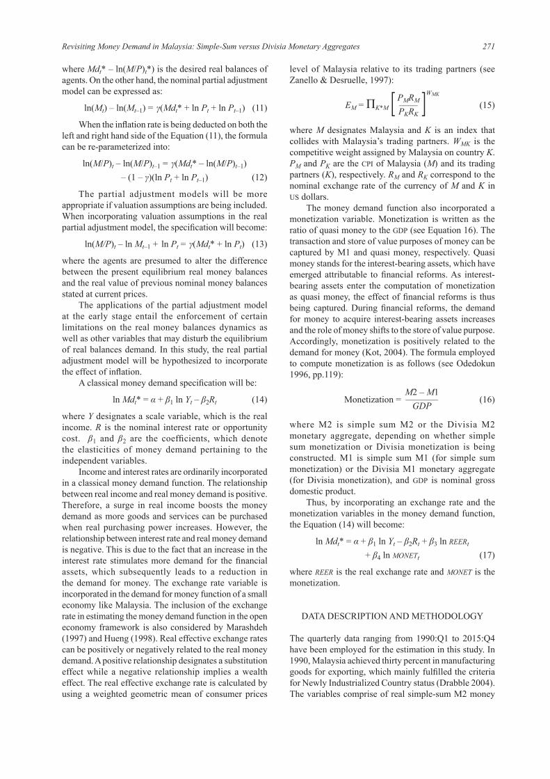
where Mdt* – ln(M/P)t*) is the desired real balances of agents. On the other hand, the nominal partial adjustment model can be expressed as:

ln(Mt) – ln(Mt–1) = γ(Mdt* + ln Pt + ln Pt–1) (11)

When the inflation rate is being deducted on both the left and right hand side of the Equation (11), the formula can be re-parameterized into:

ln(M/P)t – ln(M/P)t–1 = γ(Mdt* – ln(M/P)t–1) – (1 – γ)(ln Pt + ln Pt–1) (12)

The partial adjustment models will be more appropriate if valuation assumptions are being included. When incorporating valuation assumptions in the real partial adjustment model, the specification will become:

ln(M/P)t – ln Mt–1 + ln Pt = γ(Mdt* + ln Pt) (13)

where the agents are presumed to alter the difference between the present equilibrium real money balances and the real value of previous nominal money balances stated at current prices.

The applications of the partial adjustment model at the early stage entail the enforcement of certain limitations on the real money balances dynamics as well as other variables that may disturb the equilibrium of real balances demand. In this study, the real partial adjustment model will be hypothesized to incorporate the effect of inflation.

A classical money demand specification will be:

ln Mdt* = α + β1 ln Yt – β2rt (14)

where Y designates a scale variable, which is the real income. r is the nominal interest rate or opportunity cost. β1 and β2 are the coefficients, which denote the elasticities of money demand pertaining to the independent variables.

Income and interest rates are ordinarily incorporated in a classical money demand function. The relationship between real income and real money demand is positive. Therefore, a surge in real income boosts the money demand as more goods and services can be purchased when real purchasing power increases. However, the relationship between interest rate and real money demand is negative. This is due to the fact that an increase in the interest rate stimulates more demand for the financial assets, which subsequently leads to a reduction in the demand for money. The exchange rate variable is incorporated in the demand for money function of a small economy like Malaysia. The inclusion of the exchange rate in estimating the money demand function in the open economy framework is also considered by Marashdeh (1997) and Hueng (1998). Real effective exchange rates can be positively or negatively related to the real money demand. A positive relationship designates a substitution effect while a negative relationship implies a wealth effect. The real effective exchange rate is calculated by using a weighted geometric mean of consumer prices

level of Malaysia relative to its trading partners (see Zanello & Desruelle, 1997):

EM = Πk*M [ PMrM––––Pkrk

]WMk

(15)

where M designates Malaysia and k is an index that collides with Malaysia’s trading partners. WMk is the competitive weight assigned by Malaysia on country k. PM and Pk are the CPI of Malaysia (M) and its trading partners (k), respectively. rM and rk correspond to the nominal exchange rate of the currency of M and k in US dollars.

The money demand function also incorporated a monetization variable. Monetization is written as the ratio of quasi money to the GDP (see Equation 16). The transaction and store of value purposes of money can be captured by M1 and quasi money, respectively. Quasi money stands for the interest-bearing assets, which have emerged attributable to financial reforms. As interest-bearing assets enter the computation of monetization as quasi money, the effect of financial reforms is thus being captured. During financial reforms, the demand for money to acquire interest-bearing assets increases and the role of money shifts to the store of value purpose. Accordingly, monetization is positively related to the demand for money (Kot, 2004). The formula employed to compute monetization is as follows (see Odedokun 1996, pp.119):

Monetization = M2 – M1–––––––

GDP (16)

where M2 is simple sum M2 or the Divisia M2 monetary aggregate, depending on whether simple sum monetization or Divisia monetization is being constructed. M1 is simple sum M1 (for simple sum monetization) or the Divisia M1 monetary aggregate (for Divisia monetization), and GDP is nominal gross domestic product.

Thus, by incorporating an exchange rate and the monetization variables in the money demand function, the Equation (14) will become:

ln Mdt* = α + β1 ln Yt – β2rt + β3 ln rEErt + β4 ln MONETt (17)

where rEEr is the real exchange rate and MONET is the monetization.

DATA DESCRIPTION AND METHODOLOGY

The quarterly data ranging from 1990:Q1 to 2015:Q4 have been employed for the estimation in this study. In 1990, Malaysia achieved thirty percent in manufacturing goods for exporting, which mainly fulfilled the criteria for Newly Industrialized Country status (Drabble 2004). The variables comprise of real simple-sum M2 money


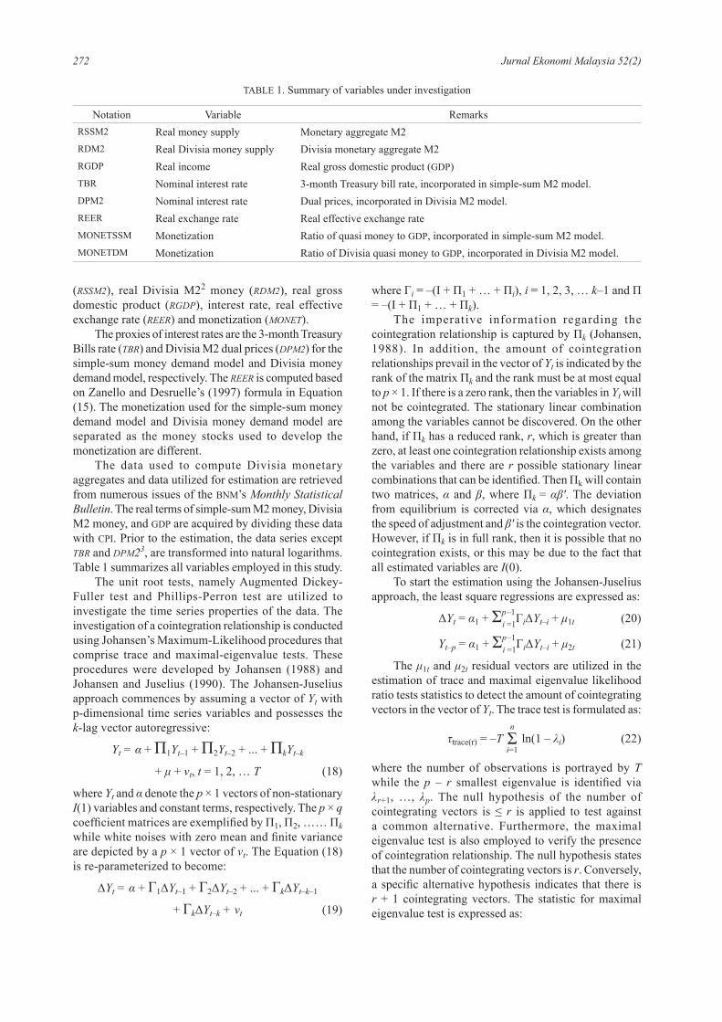
(rSSM2), real Divisia M22 money (rDM2), real gross domestic product (rGDP), interest rate, real effective exchange rate (rEEr) and monetization (MONET).

The proxies of interest rates are the 3-month Treasury Bills rate (tbr) and Divisia M2 dual prices (DPM2) for the simple-sum money demand model and Divisia money demand model, respectively. The rEEr is computed based on Zanello and Desruelle’s (1997) formula in Equation (15). The monetization used for the simple-sum money demand model and Divisia money demand model are separated as the money stocks used to develop the monetization are different.

The data used to compute Divisia monetary aggregates and data utilized for estimation are retrieved from numerous issues of the BNM’s Monthly Statistical bulletin. The real terms of simple-sum M2 money, Divisia M2 money, and GDP are acquired by dividing these data with CPI. Prior to the estimation, the data series except tbr and DPM23, are transformed into natural logarithms. Table 1 summarizes all variables employed in this study.

The unit root tests, namely Augmented Dickey-Fuller test and Phillips-Perron test are utilized to investigate the time series properties of the data. The investigation of a cointegration relationship is conducted using Johansen’s Maximum-Likelihood procedures that comprise trace and maximal-eigenvalue tests. These procedures were developed by Johansen (1988) and Johansen and Juselius (1990). The Johansen-Juselius approach commences by assuming a vector of Yt with p-dimensional time series variables and possesses the k-lag vector autoregressive:

Yt = α + Π1Yt–1 + Π2Yt–2 + ... + ΠkYt–k

+ μ + vt, t = 1, 2, … t (18)

where Yt and α denote the p × 1 vectors of non-stationary I(1) variables and constant terms, respectively. The p × q coefficient matrices are exemplified by Π1, Π2, …… Πk while white noises with zero mean and finite variance are depicted by a p × 1 vector of vt. The Equation (18) is re-parameterized to become:

ΔYt = α + Γ1ΔYt–1 + Γ2ΔYt–2 + ... + ΓkΔYt–k–1

+ ΓkΔYt–k + vt (19)

where Γi = –(Ι + Π1 + … + Πi), i = 1, 2, 3, … k–1 and Π = –(Ι + Π1 + … + Πk).

The imperative information regarding the cointegration relationship is captured by Πk (Johansen, 1988). In addition, the amount of cointegration relationships prevail in the vector of Yt is indicated by the rank of the matrix Πk and the rank must be at most equal to p × 1. If there is a zero rank, then the variables in Yt will not be cointegrated. The stationary linear combination among the variables cannot be discovered. On the other hand, if Πk has a reduced rank, r, which is greater than zero, at least one cointegration relationship exists among the variables and there are r possible stationary linear combinations that can be identified. Then Πk will contain two matrices, α and β, where Πk = αβ'. The deviation from equilibrium is corrected via α, which designates the speed of adjustment and β' is the cointegration vector. However, if Πk is in full rank, then it is possible that no cointegration exists, or this may be due to the fact that all estimated variables are I(0).

To start the estimation using the Johansen-Juselius approach, the least square regressions are expressed as:

ΔYt = α1 + Σpi

–1=1ΓiΔYt–i + μ1t (20)

Yt–p = α1 + Σpi

–1=1ΓiΔYt–i + μ2t (21)

The μ1t and μ2t residual vectors are utilized in the estimation of trace and maximal eigenvalue likelihood ratio tests statistics to detect the amount of cointegrating vectors in the vector of Yt. The trace test is formulated as:

τtrace(r) = –t n

Σi=1

ln(1 – λi) (22)

where the number of observations is portrayed by t while the p – r smallest eigenvalue is identified via λr+1, …, λp. The null hypothesis of the number of cointegrating vectors is ≤ r is applied to test against a common alternative. Furthermore, the maximal eigenvalue test is also employed to verify the presence of cointegration relationship. The null hypothesis states that the number of cointegrating vectors is r. Conversely, a specific alternative hypothesis indicates that there is r + 1 cointegrating vectors. The statistic for maximal eigenvalue test is expressed as:

TABLE 1. Summary of variables under investigation

Notation Variable RemarksRSSM2 Real money supply Monetary aggregate M2RDM2 Real Divisia money supply Divisia monetary aggregate M2RGDP Real income Real gross domestic product (GDP)TBR Nominal interest rate 3-month Treasury bill rate, incorporated in simple-sum M2 model.DPM2 Nominal interest rate Dual prices, incorporated in Divisia M2 model.REER Real exchange rate Real effective exchange rateMONETSSM Monetization Ratio of quasi money to GDP, incorporated in simple-sum M2 model.MONETDM Monetization Ratio of Divisia quasi money to GDP, incorporated in Divisia M2 model.


τmax(r,r+1) = –t ln(1 – λr+1) (23)

Opposed to trace test, λr+1 is used to determine the (r+t)th largest eigenvalue.

If n is the quantity of variables, the trace and maximal eigenvalue tests possess identical degree of freedom with the number of restrictions (n – r). Some results of Brownian motion theory are adopted by Johansen to achieve asymptotic distribution of the test statistics since there is a non-standard distribution of the likelihood ratio values under the null hypothesis. The critical values of Johansen (1988) do not include an intercept term or seasonal dummies. As a result, an intercept term is included in the critical values of Johansen and Juselius (1990). Among two likelihood ratio tests, trace test shows powerful estimation compared to maximal-eigenvalue test (Johansen & Juselius 1990) and thus the former test is more favorable than the latter.

If cointegration relationship prevails between the estimated variables, the estimation is carried on by applying the error-correction model (ECM) approach. This method is introduced by Engle and Granger (1987) and is used to identify the long-run and short-run effects of the explanatory variables on response variable. Error-correction term (ECT) is used to evaluate the adjustment of cointegrated variables in the short run to correct for the deviation of long-run equilibrium. The econometric model of Equation (17) based on the ECM approach is written as:

ΔMdt* = β0 + β1ΔMd*t–1 + β2ΔYt + β3Δrt + β4ΔrEErt + β5ΔMONETt + β6Ectt–1 + μt (24)

where β0 and Δ designate the intercept and the first difference, respectively. β1 to β5 denote the short-run elasticities of lagged value of the variables, namely real demand for money, real income, interest rate, real effective exchange rate as well as monetization. The

coefficient of β6 depicts ECT, which holds information of long run as it is derived from the cointegrating vector. The Hannan-Quinn information criterion4 is used to select the optimal lag for the estimated model. A parsimonious ECM is derived by eliminating the insignificant coefficients successively using the general to specific technique of Hendry and Ericsson (1991).

RESULTS AND DISCUSSION

UNIT ROOT TEST RESULTS

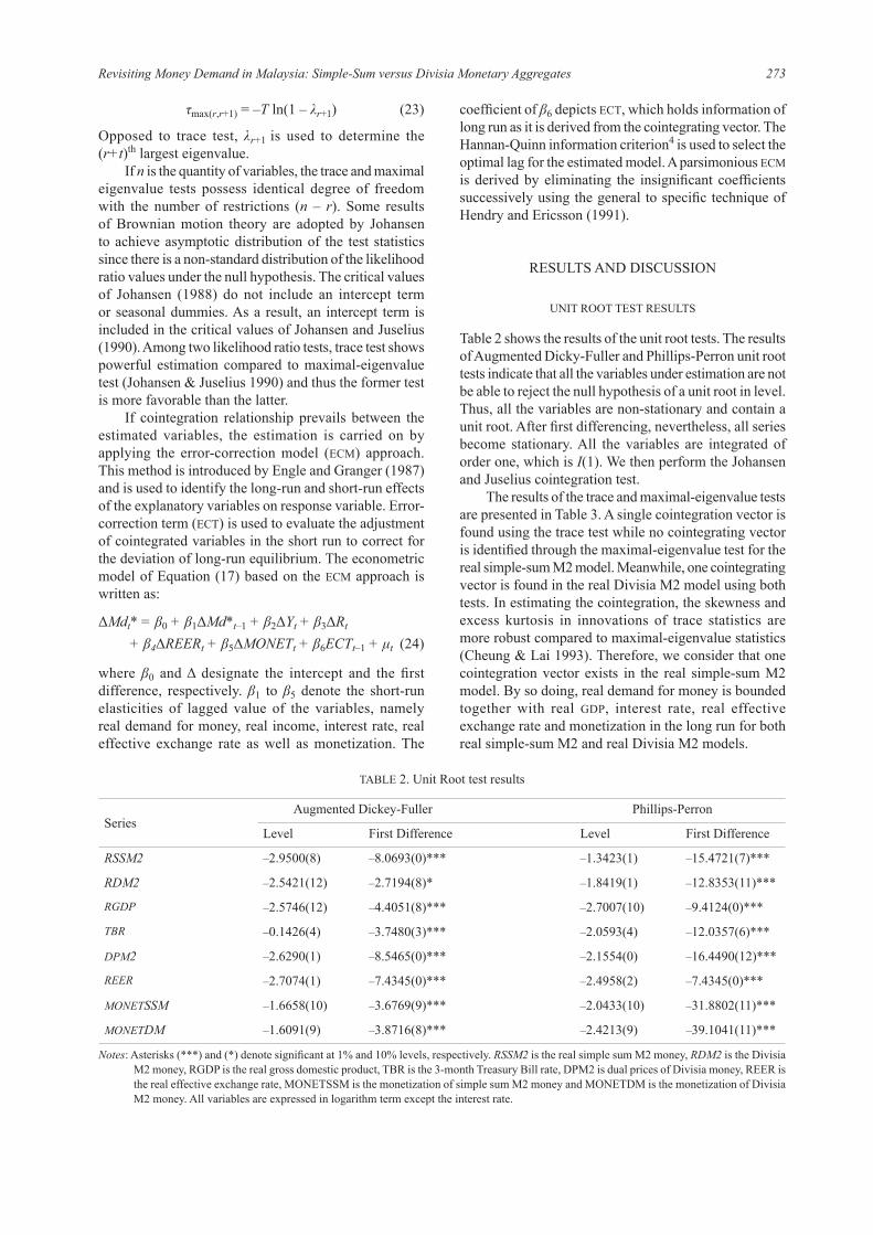
Table 2 shows the results of the unit root tests. The results of Augmented Dicky-Fuller and Phillips-Perron unit root tests indicate that all the variables under estimation are not be able to reject the null hypothesis of a unit root in level. Thus, all the variables are non-stationary and contain a unit root. After first differencing, nevertheless, all series become stationary. All the variables are integrated of order one, which is I(1). We then perform the Johansen and Juselius cointegration test.

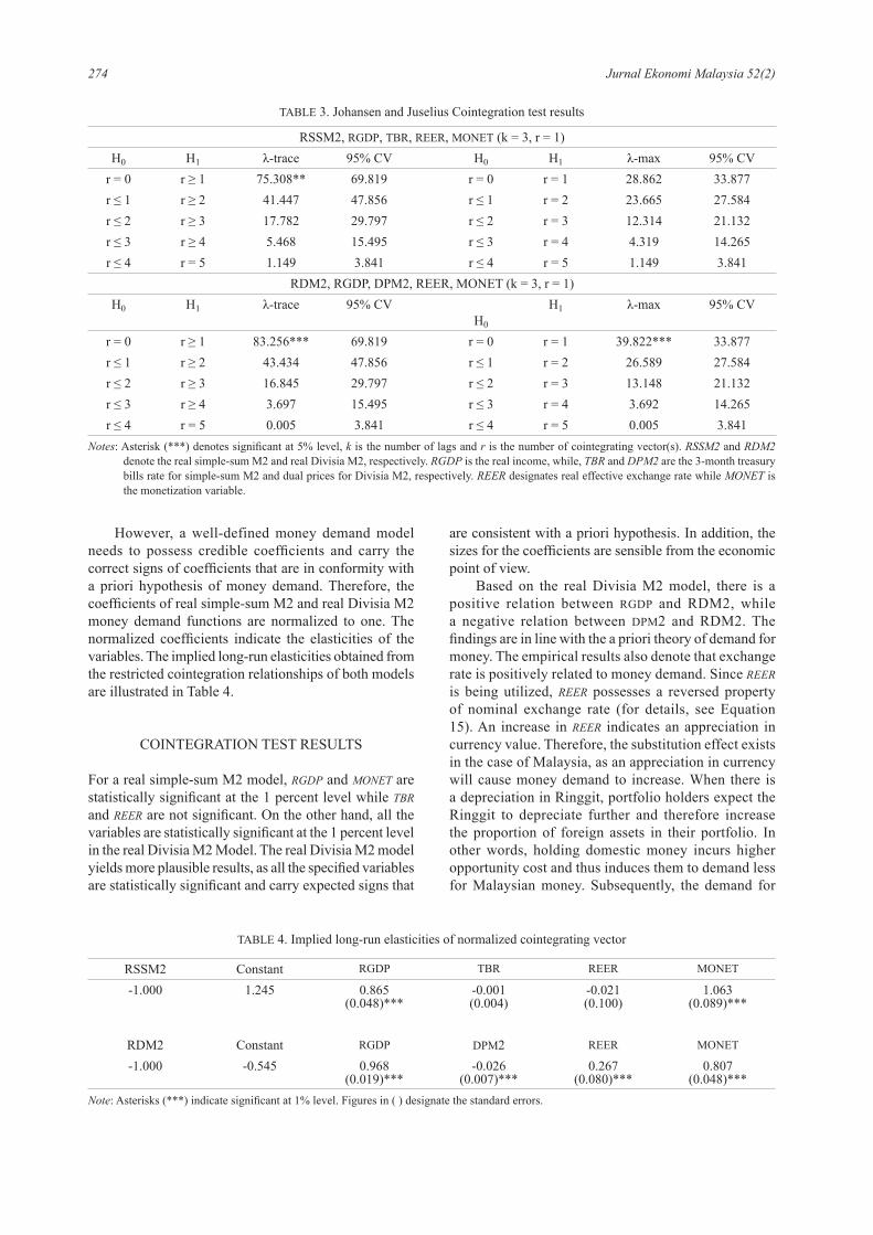
The results of the trace and maximal-eigenvalue tests are presented in Table 3. A single cointegration vector is found using the trace test while no cointegrating vector is identified through the maximal-eigenvalue test for the real simple-sum M2 model. Meanwhile, one cointegrating vector is found in the real Divisia M2 model using both tests. In estimating the cointegration, the skewness and excess kurtosis in innovations of trace statistics are more robust compared to maximal-eigenvalue statistics (Cheung & Lai 1993). Therefore, we consider that one cointegration vector exists in the real simple-sum M2 model. By so doing, real demand for money is bounded together with real GDP, interest rate, real effective exchange rate and monetization in the long run for both real simple-sum M2 and real Divisia M2 models.

TABLE 2. Unit Root test results

SeriesAugmented Dickey-Fuller Phillips-Perron

Level First Difference Level First Difference

rSSM2 –2.9500(8) –8.0693(0)*** –1.3423(1) –15.4721(7)***

rDM2 –2.5421(12) –2.7194(8)* –1.8419(1) –12.8353(11)***

rGDP –2.5746(12) –4.4051(8)*** –2.7007(10) –9.4124(0)***

tbr –0.1426(4) –3.7480(3)*** –2.0593(4) –12.0357(6)***

DPM2 –2.6290(1) –8.5465(0)*** –2.1554(0) –16.4490(12)***

rEEr –2.7074(1) –7.4345(0)*** –2.4958(2) –7.4345(0)***

MONETSSM –1.6658(10) –3.6769(9)*** –2.0433(10) –31.8802(11)***

MONETDM –1.6091(9) –3.8716(8)*** –2.4213(9) –39.1041(11)***

Notes: Asterisks (***) and (*) denote significant at 1% and 10% levels, respectively. rSSM2 is the real simple sum M2 money, rDM2 is the Divisia M2 money, RGDP is the real gross domestic product, TBR is the 3-month Treasury Bill rate, DPM2 is dual prices of Divisia money, REER is the real effective exchange rate, MONETSSM is the monetization of simple sum M2 money and MONETDM is the monetization of Divisia M2 money. All variables are expressed in logarithm term except the interest rate.


However, a well-defined money demand model needs to possess credible coefficients and carry the correct signs of coefficients that are in conformity with a priori hypothesis of money demand. Therefore, the coefficients of real simple-sum M2 and real Divisia M2 money demand functions are normalized to one. The normalized coefficients indicate the elasticities of the variables. The implied long-run elasticities obtained from the restricted cointegration relationships of both models are illustrated in Table 4.

COINTEGRATION TEST RESULTS

For a real simple-sum M2 model, rGDP and MONET are statistically significant at the 1 percent level while tbr and rEEr are not significant. On the other hand, all the variables are statistically significant at the 1 percent level in the real Divisia M2 Model. The real Divisia M2 model yields more plausible results, as all the specified variables are statistically significant and carry expected signs that

are consistent with a priori hypothesis. In addition, the sizes for the coefficients are sensible from the economic point of view.

Based on the real Divisia M2 model, there is a positive relation between RGDP and RDM2, while a negative relation between DPM2 and RDM2. The findings are in line with the a priori theory of demand for money. The empirical results also denote that exchange rate is positively related to money demand. Since rEEr is being utilized, rEEr possesses a reversed property of nominal exchange rate (for details, see Equation 15). An increase in rEEr indicates an appreciation in currency value. Therefore, the substitution effect exists in the case of Malaysia, as an appreciation in currency will cause money demand to increase. When there is a depreciation in Ringgit, portfolio holders expect the Ringgit to depreciate further and therefore increase the proportion of foreign assets in their portfolio. In other words, holding domestic money incurs higher opportunity cost and thus induces them to demand less for Malaysian money. Subsequently, the demand for

TABLE 4. Implied long-run elasticities of normalized cointegrating vector

RSSM2 Constant RGDP TBR REER MONET

-1.000 1.245 0.865(0.048)***

-0.001(0.004)

-0.021(0.100)

1.063(0.089)***

RDM2 Constant RGDP DPM2 REER MONET

-1.000 -0.545 0.968(0.019)***

-0.026(0.007)***

0.267(0.080)***

0.807(0.048)***

Note: Asterisks (***) indicate significant at 1% level. Figures in ( ) designate the standard errors.

TABLE 3. Johansen and Juselius Cointegration test results

RSSM2, RGDP, TBR, REER, MONET (k = 3, r = 1)H0 H1 λ-trace 95% CV H0 H1 λ-max 95% CV

r = 0 r ≥ 1 75.308** 69.819 r = 0 r = 1 28.862 33.877r ≤ 1 r ≥ 2 41.447 47.856 r ≤ 1 r = 2 23.665 27.584r ≤ 2 r ≥ 3 17.782 29.797 r ≤ 2 r = 3 12.314 21.132r ≤ 3 r ≥ 4 5.468 15.495 r ≤ 3 r = 4 4.319 14.265r ≤ 4 r = 5 1.149 3.841 r ≤ 4 r = 5 1.149 3.841

RDM2, RGDP, DPM2, REER, MONET (k = 3, r = 1)H0 H1 λ-trace 95% CV

H0

H1 λ-max 95% CV

r = 0 r ≥ 1 83.256*** 69.819 r = 0 r = 1 39.822*** 33.877r ≤ 1 r ≥ 2 43.434 47.856 r ≤ 1 r = 2 26.589 27.584r ≤ 2 r ≥ 3 16.845 29.797 r ≤ 2 r = 3 13.148 21.132r ≤ 3 r ≥ 4 3.697 15.495 r ≤ 3 r = 4 3.692 14.265r ≤ 4 r = 5 0.005 3.841 r ≤ 4 r = 5 0.005 3.841

Notes: Asterisk (***) denotes significant at 5% level, k is the number of lags and r is the number of cointegrating vector(s). rSSM2 and rDM2 denote the real simple-sum M2 and real Divisia M2, respectively. rGDP is the real income, while, tbr and DPM2 are the 3-month treasury bills rate for simple-sum M2 and dual prices for Divisia M2, respectively. rEEr designates real effective exchange rate while MONET is the monetization variable.


Ringgit lessens as well. The findings are consistent with Marashdeh (1997) and Chaisrisawatsuk et al. (2004) that a currency substitution effect existed in Malaysia. Substitution effect also was found in the study of Bahmani-Oskooee (2002) in which the depreciation of currency led to a fall in money demand in Hong Kong. Conversely, monetization is positively related to money demand. Therefore, the interest-bearing assets surge induces higher demand for money to acquire them. Ahmad (2001) also found that acceleration in monetization grounds greater demand for money.

ERROR-CORRECTION MODEL AND GRANGER-CAUSALITY TEST RESULTS

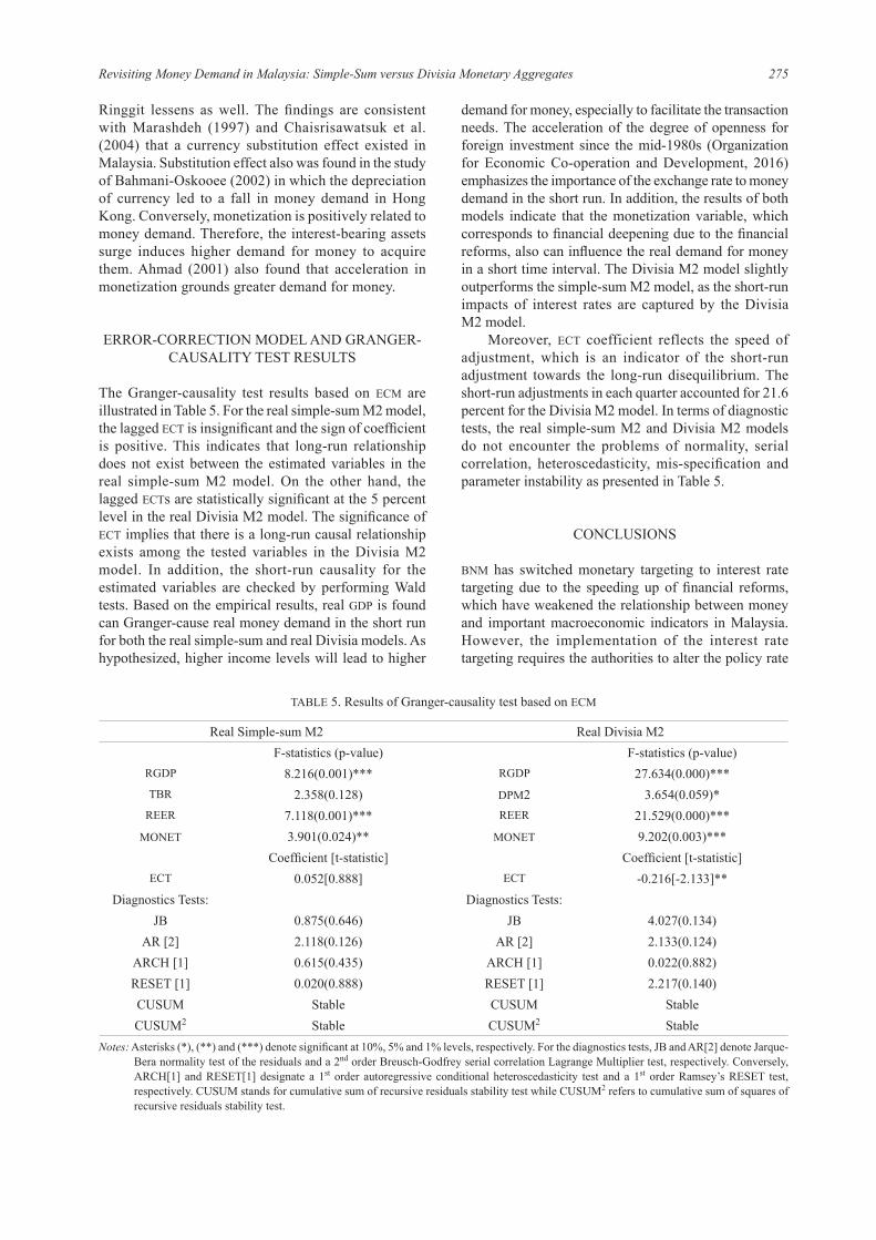
The Granger-causality test results based on ECM are illustrated in Table 5. For the real simple-sum M2 model, the lagged ECT is insignificant and the sign of coefficient is positive. This indicates that long-run relationship does not exist between the estimated variables in the real simple-sum M2 model. On the other hand, the lagged ECTs are statistically significant at the 5 percent level in the real Divisia M2 model. The significance of ECT implies that there is a long-run causal relationship exists among the tested variables in the Divisia M2 model. In addition, the short-run causality for the estimated variables are checked by performing Wald tests. Based on the empirical results, real GDP is found can Granger-cause real money demand in the short run for both the real simple-sum and real Divisia models. As hypothesized, higher income levels will lead to higher

demand for money, especially to facilitate the transaction needs. The acceleration of the degree of openness for foreign investment since the mid-1980s (Organization for Economic Co-operation and Development, 2016) emphasizes the importance of the exchange rate to money demand in the short run. In addition, the results of both models indicate that the monetization variable, which corresponds to financial deepening due to the financial reforms, also can influence the real demand for money in a short time interval. The Divisia M2 model slightly outperforms the simple-sum M2 model, as the short-run impacts of interest rates are captured by the Divisia M2 model.

Moreover, ECT coefficient reflects the speed of adjustment, which is an indicator of the short-run adjustment towards the long-run disequilibrium. The short-run adjustments in each quarter accounted for 21.6 percent for the Divisia M2 model. In terms of diagnostic tests, the real simple-sum M2 and Divisia M2 models do not encounter the problems of normality, serial correlation, heteroscedasticity, mis-specification and parameter instability as presented in Table 5.

CONCLUSIONS

BNM has switched monetary targeting to interest rate targeting due to the speeding up of financial reforms, which have weakened the relationship between money and important macroeconomic indicators in Malaysia. However, the implementation of the interest rate targeting requires the authorities to alter the policy rate

TABLE 5. Results of Granger-causality test based on ECM

Real Simple-sum M2 Real Divisia M2F-statistics (p-value) F-statistics (p-value)

RGDP 8.216(0.001)*** RGDP 27.634(0.000)***TBR 2.358(0.128) DPM2 3.654(0.059)*

REER 7.118(0.001)*** REER 21.529(0.000)***MONET 3.901(0.024)** MONET 9.202(0.003)***

Coefficient [t-statistic] Coefficient [t-statistic]ECT 0.052[0.888] ECT -0.216[-2.133]**

Diagnostics Tests: Diagnostics Tests:JB 0.875(0.646) JB 4.027(0.134)

AR [2] 2.118(0.126) AR [2] 2.133(0.124)ARCH [1] 0.615(0.435) ARCH [1] 0.022(0.882)RESET [1] 0.020(0.888) RESET [1] 2.217(0.140)CUSUM Stable CUSUM Stable CUSUM2 Stable CUSUM2 Stable

Notes: Asterisks (*), (**) and (***) denote significant at 10%, 5% and 1% levels, respectively. For the diagnostics tests, JB and AR[2] denote Jarque-Bera normality test of the residuals and a 2nd order Breusch-Godfrey serial correlation Lagrange Multiplier test, respectively. Conversely, ARCH[1] and RESET[1] designate a 1st order autoregressive conditional heteroscedasticity test and a 1st order Ramsey’s RESET test, respectively. CUSUM stands for cumulative sum of recursive residuals stability test while CUSUM2 refers to cumulative sum of squares of recursive residuals stability test.


recurrently. Alternatively, the authorities may consider monetary targeting, which provides ease of control of monetary aggregates, provided the money demand function is stable. However, financial liberalization has greatly affected the stability of demand for money. Thus, the demand for money function in Malaysia has been examined in this study by considering the effect of the financial development. Another alternative measurement for money, namely the Divisia monetary aggregate is constructed, and a monetization variable is included in the function. The money demand function was estimated by using the Johansen and Juselius cointegration test and error correction model. The prominent performance of the Divisia M2 monetary aggregate is confirmed via the empirical results of the demand for money estimation. The derived money demand function is plausible using Divisia M2. The model is also robust as it passed all the diagnostic tests. The findings of Dahalan et al. (2005), Leong et al. (2010), and Sarwar et al. (2010) also support the empirical results of this study that the performance of Divisia M2 is superior than its simple-sum counterpart in the money demand function estimation. Moreover, monetization appears as an important variable that contributes to a stable money demand due to the hastening of financial development in Malaysia in recent years. Therefore, the presence of a stable Divisia M2 money demand has reassured the usefulness of monetary targeting for monetary policy purposes. The significance of Divisia M2 money may boost the possibility of reverting back to monetary targeting with the presence of a stable money demand function. In addition, the Central Bank may consider Divisia monetary aggregates as an alternative money supply apart from the simple-sum money supply. For instance, the Federal Reserve Bank of St. Louis has published the data of Divisia monetary aggregates as alternative official money supply. Furthermore, due to the financial reforms, financial development variables such as monetization become significant in determining the money demand in Malaysia. In this study, a parsimonious model can be derived by incorporating a monetization variable.

ACKNOWLEDGEMENT

Financial support from Centre for Business, Economics and Finance Forecasting (BEFfore) in Universiti Malaysia Sarawak (UNIMAS) via top-down research grant: 03(TD04)/1054/2013(02) is gratefully acknowledged.

NOTES

1 The discussion in this section follows Hoffman and Rasche (1996).

2 Only simple sum and Divisia M2 monies are tested as the option of monetary aggregates is arbitrary (Goldfeld and Sichel, 1990). M2 is considered more appropriate for a broader money definition (Tseng and Corker, 1991).

Moreover, Valadkhani and Alauddin (2003) contended that there is increased agreement among economists to conceive M2 as appropriate alternative of monetary aggregate.

3 Although all variables are required to be measured in logs, due to the nature of nominal interest rates, it is expressed in percentage per annum, it does not require the transformation to the log (Dreger et al., 2016). There is no exponential trend to linearize.

4 The consistency in estimation for the order of an autoregressive model is found to be strong using this approach (Hannan and Quinn, 1979).

REFERENCES

Ahmad, M. 2001. Demand for money in Bangladesh: An econometric investigation into some basic issue. the Indian Economic Journal 48(1): 84–89.

Almekinders, G., Fukuda, S., Mourmouras, A., Zhou, J. & Zhou, Y.S. 2015. ASEAN Financial Integration. International Monetary Fund Working Paper No. WP/15/34.

Anderson, R.G. & Jones, B.E. 2011. A comprehensive revision of the U.S. monetary services (divisia) indexes. Federal Reserve Bank of St. Louis Review 93(5): 325–359.

Anderson, R.G., Jones, B.E. & Nesmith, T.D. 1997. Building new monetary services indexes: Concepts, data and methods. Federal Reserve Bank of St. Louis Review 79(1): 53–82.

Bahmani-Oskooee, M. 2002. Long-run demand for money in Hong Kong: An application of the ARDL model. International Journal of business and Economics 1(2): 147–155.

Bank Negara Malaysia. 1999. the central bank and the Financial System in Malaysia. Kuala Lumpur: Bank Negara Malaysia.

Bank Negara Malaysia. 2011. Financial Sector blueprint 2011-2020. Kuala Lumpur: Bank Negara Malaysia.

Barnett, W.A. & Tang, B. 2016. Chinese divisia monetary index and GDP nowcasting. Open Economies Review 27(5): 825–849.

Barnett, W.A. 1978. The user cost of money. Economics Letters 1(2): 145–149.

Barnett, W.A. 1980. Economic monetary aggregates: An application of index number and aggregation theory. Journal of Econometrics 14(1): 11–48.

Binner, J.M., Fielding, A. & Mullineux, A.W. 1999. Divisia money in a composite leading indicator of inflation. Applied Economics 31(8): 1021–1031.

Carlson, J.B. & Parrott, E. 1991. The Demand for M2, opportunity cost, and financial change. Economic Review 27(2): 2–11.

Chaisrisawatsuk, S., Sharma, S.C. & Chowdhury, A. 2004. Money demand stability under currency substitution: Some recent evidence. Applied Financial Economics 14(1): 19–27.

Chen, W. & Nautz, D. 2015. the Information content of Monetary Statistics for the Great recession: Evidence from Germany. Humboldt-Universität zu Berlin, School of Business and Economics, Sonderforschungsbereich (SFB) 649 Discussion Paper No. 2015–027.

Cheung, Y.W. & Lai, K.S. 1993. Finite-sample sizes of Johansen’s likelihood ratio tests for cointegration. Oxford bulletin of Economics and Statistics 55(3): 313–328.


Chow, G. 1966. On the short-run and long-run demand for money. Journal of Political Economy 74: 111–131.

Dahalan, J., Sharma, S.C. & Sylwester, K. 2005. Divisia monetary aggregates and money demand for Malaysia. Journal of Asian Economics 15(6): 1137–1153.

Daquila, T.C. 2007. the transformation of Southeast Asian Economies. New York: Nova Science Publishers.

Darrat, A.F., Chopin, M.C. & Lobo, B.J. 2005. Money and macroeconomic performance: Revisiting divisia money. Review of Financial Economics 14(2): 93–101.

Darvas, Z. 2014. Does Money Matter in the Euro area? Evidence from a New Divisia Index. Bruegel Working Paper No. 2014/12.

Drabble, J.H. 2004. The economic history of Malaysia. In EH.Net Encyclopedia, ed. R. Whaples. Retrieved from http://eh.net/encyclopedia/economic-history-of-malaysia/.

Dreger, C., Gerdesmeier, D. & Roffia, B. 2016. Re-vitalizing Money Demand in the Euro area: Still Valid at the Zero Lower Bound. DIW Berlin Discussion Paper No. 1606.

Engle, R.F. & Granger, C.W.J. 1987. Co-integration and error correction: Representation, estimation, and testing. Econometrica 55(2): 251–276.

Goldfeld, S.M. & Sichel, D.E. 1990. The demand for money. In Handbook of monetary economics, eds. B.M. Friendman & H. Hahn. 229-356. Amsterdam: Elsevier Science.

Habibullah, M.S. 1999a. Rationale for Divisia monetary aggregates in ‘deregulated’ Asian developing countries. In Divisia monetary aggregates and economic activities in Asian developing economics, ed. M.S. Habibullah. 67–111. Aldershot: Ashgate Publishing Limited.

Habibullah, M.S. 1999b. The P-Star model approach: Linking divisia money and prices in the Asian countries. In Divisia monetary aggregates and economic activities in Asian developing economics, ed. M.S. Habibullah. 112-140. Aldershot: Ashgate Publishing Limited.

Hannan, E.J. & Quinn, B.G. 1979. The determination of the order of an autoregression. Journal of the royal Statistical Society, Series B 41: 190–195.

Hendrickson, J.R. 2013. Redundancy or mismeasurement: A reappraisal of money. Macroeconomic Dynamics 18: 1437–1465.

Hendry, D.F. & Ericsson, N.R. 1991. An econometric analysis of UK money demand in ‘monetary trends in the United States and the United Kingdom by Milton Friedman and Anna J. Schwartz’. American Economic Review 81(1): 8–38.

Hiew, L.C., Puah, C.H. & Habibullah, M.S. 2013. the role of Advertising Expenditure in Measuring Indonesia’s Money Demand Function. MPRA Paper No. 50223.

Hoffman, D.L. & Rasche, R. H. 1996. Aggregate Money Demand Functions: Empirical Applications in cointegrated Systems. Massachusetts: Kluwer Academic Publishers.

Hueng, C.J. 1998. The demand for money in an open economy: Some evidence for Canada. the North American Journal of Economics and Finance 9(1): 15–31.

Hussain, H. & Liew, V.K.S. 2006. Money demand in Malaysia: Further empirical evidence. the IUP Journal of Applied Economics 6: 17–27.

Johansen, S. & Juselius, K. 1990. Maximum likelihood estimation and inference on cointegration - With applications to the demand for money. Oxford Bulletin of Economics & Statistics 52(2): 169–210.

Johansen, S. 1988. Statistical analysis of cointegration vectors. Journal of Economic Dynamics and control 12(2-3): 231–254.

Kamaruddin, A.A. & Khalid, N. 2016. Fungsi permintaan wang di malaysia menggunakan pendekatan simetri dan asimetri: Perbandingan indeks penjumlahan mudah dan divisia. Jurnal Ekonomi Malaysia 50(2): 181–196.

Karim, Z.A. & Karim, B.A. 2014. Interest Rates Targeting of Monetary Policy: An Open Economy SVAR Study of Malaysia. Gadjah Mada International Journal of business 16(1): 1–23.

Khainga, D. 2014. Divisia Monetary Aggregates and Demand for Money in kenya. Africa Growth Initiative Working Paper No. 13.

Kot, A. 2004. The impact of monetization on the money demand in Poland. Makroekonomia July: 31–37.

la Cour, L.F. 2006. The problem of measuring ‘money’: Results from an analysis of Divisia monetary aggregates for Denmark. In Money, measurement and computation, eds. M.T. Belongia & J.M. Binner. 185-210. New York: Palgrave MacMillan.

Leong, C.M., Puah, C.H., Shazali, A.M. & Lau, E. 2010. Testing the effectiveness of monetary policy in Malaysia using alternative monetary aggregation. Margin-the Journal of Applied Economic research 4(3): 321–338.

Lynch, D. 1996. Measuring financial sector development: A study of selected Asia-Pacific countries. the Developing Economies XXXIV(1): 3–33.

Marashdeh, O. 1997. the demand of money in an open economy: the case of Malaysia. Paper presented at the Southern Finance Association Annual Meeting, 19-22 November, Baltimore, Maryland.

Martin, C. & Milas, C. 2010. Financial market liquidity and the financial crisis: An assessment using UK data. International Finance 13(3): 443–459.

Neupauerová, M. & Vravec, J. 2007. Monetary strategies from the perspective of intermediate objectives. PANOECONOMICUS 2: 219-233.

Noman, A.H.M., Gee, C.S. & Isa, C.R. 2017. Does competition improve financial stability of the banking sector in ASEAN countries? An empirical analysis. PLoS ONE 12(5): e0176546.

Odedokun, M.O. 1996. Financial indicators and economic efficiency in developing countries. In Financial development and economic growth: Theory and experiences from developing countries, eds. N. Hermes & R. Lensink. 115-137. London: Routledge.

Organization for Economic Co-operation and Development. 2016. OECD Economic Surveys: Malaysia 2016: Economic Assessment. Paris: OECD Publishing.

Puah, C.H. & Hiew, L.C. 2010. Financial liberalization, weighted monetary aggregates and money demand in Indonesia. Labuan Bulletin of International Business & Finance 8: 76–93.

Puah, C.H., Habibullah, M.S., Lau, E. & Shazali, A.M. 2006. Testing long run monetary neutrality in Malaysia: Revisiting divisia money. Journal of International business and Economics VI(1): 110–115.

Sarwar, H., Hussain, Z. & Sarwar, M. 2010. Money demand function for Pakistan (Divisia Approach). Pakistan Economic and Social Review 48(1): 1–20.


Schunk, D.L. 2001. The relative forecasting performance of the divisia and simple sum monetary aggregates. Journal of Money, Credit and Banking 33(2): 272–283.

Sianturi, R. H., Tanjung, A. F., Leong, C. M., Puah, C. H. & Brahmana, R. K. 2017. Financial liberalization and divisia money demand in Indonesia. Advanced Science Letters 23(4): 3155–3158.

Sriram, S.S. 2002. Determinants and stability of demand for M2 in Malaysia. Journal of Asian Economics 13(3): 337–356.

Tang, M.M.J., Puah, C.H. & Liew, V.K.S. 2015a. The interest rate pass-through in Malaysia: An analysis on asymmetric adjustment. International Journal of Economics and Management 9(2): 370–381.

Tang, M.M.J., Puah, C.H., Affendy Arip, M. & Dayang Affizah, A.M. 2015b. Forecasting performance of the p-star model: The case of Indonesia. Journal of International business and Economics 15(2): 7–12.

Thornton, D.L. & Yue, P. 1992. An extended series of divisia monetary aggregates. Federal reserve bank of St. Louis Review, November/December: 35–52.

Treichel, V. 1997. broad Money Demand and Monetary Policy in tunisia. International Monetary Fund Working Paper No. WP/97/22.

Tseng, W. & Corker, R. 1991. Financial Liberalization, Money Demand, and Monetary Policy in Asian Countries. Washington, D.C.: International Monetary Fund.

Valadkhani, A. & Alauddin, M. 2003. Demand for M2 in Developing countries: An Empirical Panel Investigation. Discussion Papers in Economics, Finance and International Competitiveness No. 149.

Wihardja, M.M. 2013. Financial Integration challenges in ASEAN beyond 2015. ERIA Discussion Paper Series No. ERIA-DP-2013–27.

Zanello, A. & Desruelle, D. 1997. A Primer on the IMF’s Information Notice System. IMF Working Paper WP/97/71.

Chin-Hong Puah*Faculty of Economics and BusinessUniversiti Malaysia Sarawak94300 Kota Samarahan Sarawak MALAYSIA E-mail: [email protected]

Choi-Meng LeongLot 2864 (P/L 1319)Block 7 Muara Tebas Land District Isthmus Tanjong Seberang Pending Point Sejingkat 93450 Kuching SarawakMALAYSIA E-mail: [email protected]

Abu Mansor ShazaliFaculty of Economics and BusinessUniversiti Malaysia Sarawak94300 Kota Samarahan Sarawak MALAYSIA E-mail: [email protected]

Evan LauFaculty of Economics and BusinessUniversiti Malaysia Sarawak94300 Kota Samarahan Sarawak MALAYSIA E-mail: [email protected]

*Corresponding author

revisiting money demand in malaysia: simple-sum versus ...2)/jeko_52(2)-21.pdf · oleh itu, kajian...

Documents