Sains Malaysiana 47(3)(2018): 635–643 http://dx.doi.org/10.17576/jsm-2018-4703-25

Parallel Based Support Vector Regression for Empirical Modeling of Nonlinear Chemical Process Systems

(Regresi Vektor Sokongan Berdasarkan Selari untuk Pemodelan Empirikal Sistem Proses Kimia Nonlinear)

HASLINDA ZABIRI*, RAMASAMY MARAPPAGOUNDER & NASSER M. RAMLI

ABSTRACT

In this paper, a support vector regression (SVR) using radial basis function (RBF) kernel is proposed using an integrated parallel linear-and-nonlinear model framework for empirical modeling of nonlinear chemical process systems. Utilizing linear orthonormal basis filters (OBF) model to represent the linear structure, the developed empirical parallel model is tested for its performance under open-loop conditions in a nonlinear continuous stirred-tank reactor simulation case study as well as a highly nonlinear cascaded tank benchmark system. A comparative study between SVR and the parallel OBF-SVR models is then investigated. The results showed that the proposed parallel OBF-SVR model retained the same modelling efficiency as that of the SVR, whilst enhancing the generalization properties to out-of-sample data.

Keywords: Empirical modeling; linear and nonlinear models; nonlinear system; OBF; SVR

ABSTRAK

Di dalam kertas ini, sebuah regresi vektor sokongan (SVR) yang menggunakan fungsi asas jejarian (RBF) dicadangkan menggunakan sebuah model rangka kerja linear dan tidak linear selari bersepadu untuk pemodelan empirik sistem pemprosesan kimia tidak linear. Dengan menggunakan model penapis asas ortonormal (OBF) untuk mewakili struktur linear, model selari empirik yang terbentuk seterusnya diuji prestasinya di bawah keadaan kitaran-terbuka dalam sebuah kajian kes simulasi reaktor tangki aduk berterusan (CSTR) yang tidak selari dan juga sistem penanda aras tangka sebaran tidak linear tertinggi. Sebuah kajian perbandingan antara model SVR dan juga model OBF-SVR selari kemudiannya dikaji dengan lebih terperinci. Keputusan menunjukkan bahawa model OBF-SVR selari yang dicadang juga telah mengekalkan kecekapan pemodelan yang sama seperti SVR, di samping memperkukuh ciri generalisasi terhadap data luaran sampel.

Kata kunci: Model linear dan tidak linear; OBF; pemodelan empirik; sistem tidak linear; SVR

INTRODUCTION

Empirical modeling, or also referred to as identification, of nonlinear systems is one of the active areas in system identification in recent years. Over the years, numerous nonlinear empirical models have been reported in literature, e.g. Volterra models (Ljung 2010; Mahmoodi 2007), artificial neural networks (Norgaard 2000), fuzzy-logic based models (Beyhan & Alci 2010), nonlinear auto regressive with exogenous input (NARX) models (Nelles 2001), some combinations of them like neuro-fuzzy models (Babuška & Verbruggen 2003), support vector machine and kernel methods of modeling (Tötterman & Toivonen 2009) and wavelet decomposition based methods (Billings 2005).One modeling technique that has been gaining popularity in the recent past is the support vector machine (SVM) (Suganyadevi & Babulal 2014; Tötterman & Toivonen 2009). Based on the structural risk minimization principle, SVM, also known as support vector regression (SVR) in the field of function approximation and regression estimation, has found increasing popularity due to the higher generalization capability of the models, guaranteed global solution and sparsity (Iplikci 2010; Lu & Sun 2009; Lu et al. 2009). SVR has distinct advantages in

solving practical problems that involve nonlinearity, small training sample, and high dimension (Wang et al. 2013). One of the attractive properties of SVR for nonlinear system identification is the use of kernels which perform nonlinear mapping to a high-dimensional feature space implicitly (Cheng & Hu 2012). The selection of the kernel functions is one of the major tasks in SVR approach as different kernels result in different performances. Several nonlinear kernel functions satisfying Mercer conditions have been proposed and the commonly employed kernel functions include linear, polynomial, radial basis function and sigmoid kernels (Cheng & Hu 2012; Iplikci 2010; Liu et al. 2010; Lu & Sun 2009; Lu et al. 2009; Shirzad et al. 2014). In particular, SVR using radial basis function (RBF) kernel is widely used for regression purposes due to its effectiveness and speed in training process (Cherkassky & Ma 2004; Wang et al. 2013; Yao et al. 2004). Linear and nonlinear models in a parallel structure, whereby residuals from the linear model are used to develop the nonlinear model to pick up the nonlinearities, provides an interesting alternative in nonlinear system identification structure (Zabiri et al. 2013). This structure relies on the fact that a nonlinear model may perform worse

636

than the linear one if it is not chosen appropriately (Nelles 2001). By developing a linear model (either using input/output data or applying first principles) in parallel with the nonlinear model such that the overall model output is determined by the sum of the linear and the nonlinear parts, the performance of the overall nonlinear model is then ensured to be either equivalent to or superior than the linear model. One such example is the parallel OBF-NN model (Zabiri et al. 2013). This paper proposes an SVR model to represent the nonlinear part in the linear-and-nonlinear (hereafter named L-NL) models in parallel. In this paper, the state-of-the-art SVR model performance is investigated and compared in both the conventional as well as in the parallel structure for identification of a simulated nonlinear system and a real plant with small data sets, as well as generalization capability to out-of-sample data. Orthonormal basis filters (OBF) (Zabiri et al. 2013) model will be developed and used in this study to represent the linear part in the parallel L-NL models. Section II outlines the SVR formulation and the corresponding hyper-parameters selection using a hybrid algorithm. In Section III, the proposed parallel L-NL model will be developed. The results of simulation case study using a nonlinear CSTR will be presented in Section IV and the development of the model for a benchmark data from a highly nonlinear cascaded tanks laboratory system will be covered in Section V. Finally conclusions are drawn and future works will be discussed.

MATERIALS AND METHODS

SUPPORT VECTOR REGRESSION AND THEIR PARAMETERS SELECTION

Given the training data:

{(x1, y1), …, (xn, yn)} ⊂ Rd × R (1)

where xi false is d-dimension vector and Rd denotes the space of the input data and y is the scalar output. The first step in SVR is to map the input x onto an m-dimensional feature space using some fixed (nonlinear) mapping and then a linear model is constructed in this feature space (Cherkassky & Ma 2004). Assume the linear model f in the feature space is in the form of,

(2)

parameterized by a set of parameters w, with gj(×), j = 1, …, m represents a set of nonlinear transformations and b is the ‘bias’ term. Vapnik’s ε-insensitive loss function is defined as (Cherkassky & Ma 2004; Smola & Schölkopf 2003; Tötterman & Toivonen 2009):

Lε(y,f(×,w)) (3)

The empirical risk is:

(4)

The goal of ε-SVR is to perform linear regression in the high-dimensional feature space using ε-insensitive loss function and at the same time reduce the model complexity by minimizing (Cherkassky & Ma 2004; Lin et al. 2008; Smola & Schölkopf 2003). This can be formulated as a convex optimization problem:

Minimize (5)

subject to

To allow for some errors as well as to ensure feasibility of the optimization problem, slack variables are introduced. Hence, the SVR formulation is the minimization of the following functional:

Minimize (6)

subject to

where C is a positive constant (regularization parameter). This optimization problem can be transformed into the dual problem (Cherkassky & Ma 2004; Lin et al. 2008; Smola & Schölkopf 2003), and its solution is given by:

(7)

where the dual variables are subject to constraints:

0 ≤ αi, (8)

The kernel function, K(×i, ×), is asymmetric function satisfying Mercer’s conditions (Cherkassky & Ma 2004). Since the SVR using radial basis function (RBF) kernel is widely used for regression purposes due to its effectiveness and speed in training process (Cherkassky & Ma 2004; Wang et al. 2013; Yao et al. 2004), RBF kernel function is considered in this paper. This kernel function, which is an SV admissible kernel (Smola & Schölkopf 2003), is represented as:

637

(9)

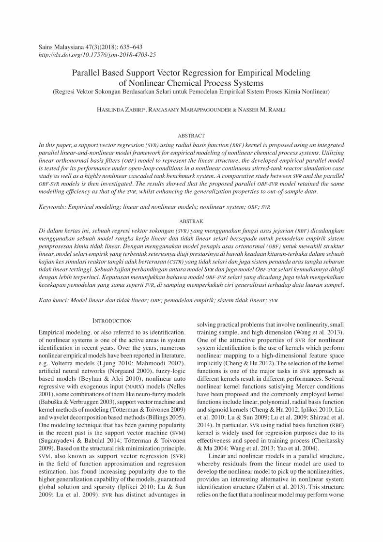
where σ is the kernel parameter. The estimation accuracy of an SVR model depends substantially on the proper selection of hyper-parameters C, ε, and kernel parameter σ (Cherkassky & Ma 2004; Lin et al. 2008; Smola & Schölkopf 2003). As reviewed in Cherkassky and Ma (2004), there are various methods proposed in the literature for selecting the three parameters. Cross-validation is one such method, however, the approach is very computational and data-intensive. Other methods include prior knowledge and/or user expertise or selection based on output data range. For the work in this paper, a hybrid approach is proposed. The hyper-parameters are selected by combining the analytical prescriptions proposed in Cherkassky and Ma (2004) and the conventional cross-validation method. The analytical prescriptions serve to provide initial guesses and cross-validation is used to fine tune the final optimal values. It was found that the combined approach significantly reduced the computational demand in the cross-validation stage, and is highly effective for our modelling purposes.In summary, the hyper-parameters are selected using a new algorithm as proposed in Figure 1. The parameters C and ε at the initial stage in Figure 1 are calculated using the analytical expressions in (10) and (11) (Cherkassky and Ma, 2004):

(10)

(11)

where and τy are the mean and standard deviation of the y values of training data, and ρ is the input noise level. Note that the algorithm in Figure 1 does not include the determination of the kernel parameter σ. For RBF kernel functions σ, it is also directly calculated using the recommendation by (Cherkassky & Ma 2004). For univariate problems, RBF width parameter is set to ρd ~ (0.1 – 0.5) * range(x). For multivariate d-dimensional problems, RBF width parameter is set to ρd ~ (0.1 – 0.5) where d input parameters are pre-scaled to [0, 1] range. The model errors in Figure 1 is defined as the root mean squared error (RMSE) between SVR estimates and the true values of the output variable for test/validation input data.

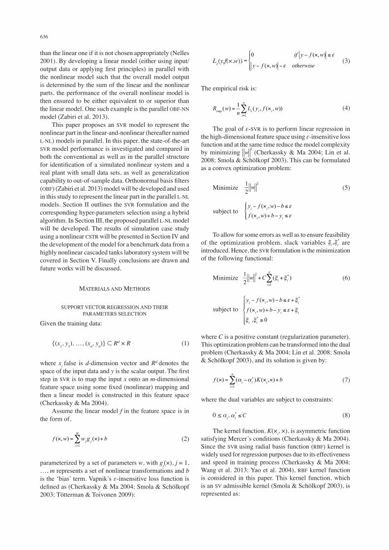
PARALLEL OBF-SVR MODEL DEVELOPMENT

MODEL STRUCTURE

To evaluate the efficacy of the proposed L-NL models in parallel using SVR, OBF model is selected as the linear part (Zabiri et al. 2013). In developing the proposed parallel OBF-SVR model, a model structure similar to OBF-NN (Zabiri et al. 2013) is adopted. In the parallel structure, the SVR model is developed using residuals generated from training data of the linear OBF. The sequential identification structure for the parallel OBF-SVR model is illustrated in Figure 2 (Zabiri et al. 2013). The linear OBF model is identified first, and the nonlinear SVR model is then developed using training data with the predicted residuals. The overall output is then expressed as the sum of the outputs of the linear and nonlinear models. A general linear model structure may be represented as:

FIGURE 1. The proposed SVR hyper-parameters selection algorithm

638

yl(k) = G(q)u(k) + e(k) (12)

where yl(k) is the output of the linear model, G(q) is the transfer function of the system, q is the forward shift operator, u(k) is the input, and refers to the system white noise. A nonlinear output error (NOE) model structure, on the other hand, is generally expressed as (Nelles 2001):

(13)

y(k) = yl(k) + ynl(k) (14)

Using (12) and (13) to represent the linear and nonlinear components, respectively, (14) can be rewritten as:

(15)

where yr refers to the predicted residuals of the linear model, . It may be emphasized here that the linear model is identified first from the input-output data and the residuals of the linear model together with the input data are used to develop the nonlinear component of the model.

The OBF linear model is expressed as:

(16)

where N is the number of orthonormal basis filters, cj are the optimal OBF model parameters, Lj(q) are the orthonormal basis filters, and q is the forward shift operator. For the nonlinear model fnl(∙), SVR as described by (7) in previous section is used.

OBF-SVR NONLINEAR IDENTIFICATION ALGORITHM

Given a set of nonlinear data to be identified [u(k), ym(k)], the algorithm can be described as follows:

Develop a parsimonious OBF model using methods described by (Tufa et al. 2011) to get yl; Calculate the predicted residuals using = ym – yl ; Develop the SVR model with x(k) = [u(k – 1), …, u(k – m), (k – 1),…, (k – m)] as inputs and as outputs of the model.

RESULTS AND DISCUSSION

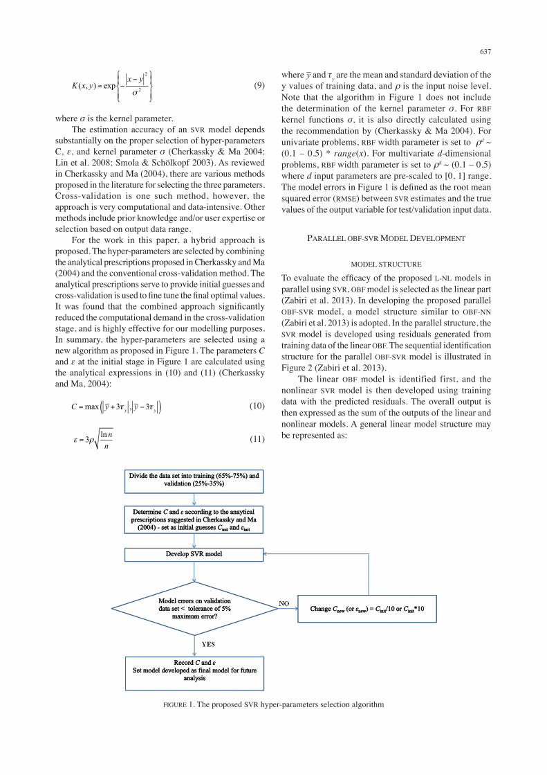
SIMULATION CASE STUDY: A NONLINEAR CSTR

Continuous stirred tank reactors (CSTR) are often encountered in industrial applications and one of the operating units widely considered in the control literature. A highly nonlinear dynamics makes CSTR a popular choice in nonlinear systems studies, and the ease of manipulating the flow of reactant or cooling liquid makes it amenable for control design purposes. The CSTR plant considered is a demo model in the Neural Network Control System Toolbox in MATLAB (MATLAB, Release 2008b) shown in Figure 3. The model equations are:

(17)

FIGURE 2. The proposed sequential identification of residual-based parallel OBF-SVR model (I: simulation configuration,

II: prediction configuration)

FIGURE 3. A catalytic continuous stirred stank reactor (CSTR)

In the equations, h(t) is the liquid level, Cb(t) is the product concentration at the output of the process, w1(t) is the flow rate of concentrated feed, and w2(t) is the flow rate of the diluted feed, Cb2. The input concentrations are set to Cb1 = 24.9 and Cb2 = 0.1. The constants associated with the rate of consumptions are kr1 = kr2 = 1. To generate the data for the identification of the nonlinear CSTR plant, Level change at random instances input signal (Norgaard 2000) is adopted. The resulting

639

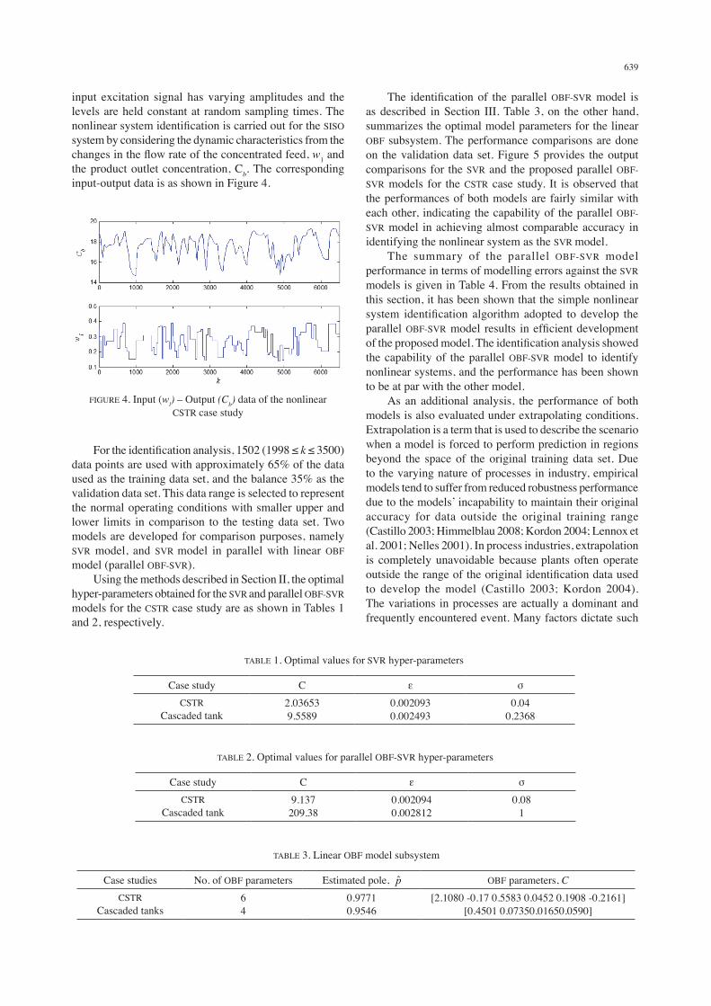
input excitation signal has varying amplitudes and the levels are held constant at random sampling times. The nonlinear system identification is carried out for the SISO system by considering the dynamic characteristics from the changes in the flow rate of the concentrated feed, w1 and the product outlet concentration, Cb. The corresponding input-output data is as shown in Figure 4.

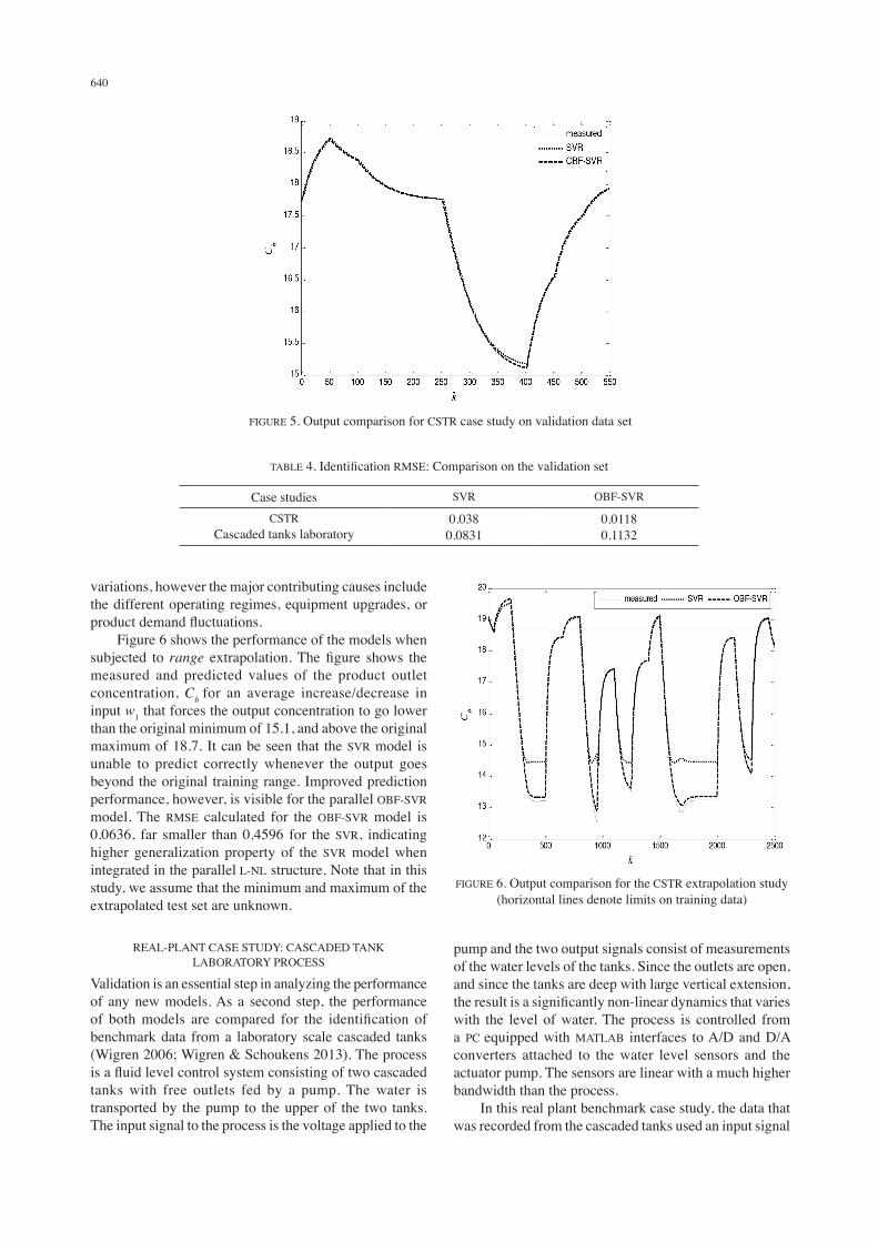
The identification of the parallel OBF-SVR model is as described in Section III. Table 3, on the other hand, summarizes the optimal model parameters for the linear OBF subsystem. The performance comparisons are done on the validation data set. Figure 5 provides the output comparisons for the SVR and the proposed parallel OBF-SVR models for the CSTR case study. It is observed that the performances of both models are fairly similar with each other, indicating the capability of the parallel OBF-SVR model in achieving almost comparable accuracy in identifying the nonlinear system as the SVR model. The summary of the parallel OBF-SVR model performance in terms of modelling errors against the SVR models is given in Table 4. From the results obtained in this section, it has been shown that the simple nonlinear system identification algorithm adopted to develop the parallel OBF-SVR model results in efficient development of the proposed model. The identification analysis showed the capability of the parallel OBF-SVR model to identify nonlinear systems, and the performance has been shown to be at par with the other model. As an additional analysis, the performance of both models is also evaluated under extrapolating conditions. Extrapolation is a term that is used to describe the scenario when a model is forced to perform prediction in regions beyond the space of the original training data set. Due to the varying nature of processes in industry, empirical models tend to suffer from reduced robustness performance due to the models’ incapability to maintain their original accuracy for data outside the original training range (Castillo 2003; Himmelblau 2008; Kordon 2004; Lennox et al. 2001; Nelles 2001). In process industries, extrapolation is completely unavoidable because plants often operate outside the range of the original identification data used to develop the model (Castillo 2003; Kordon 2004). The variations in processes are actually a dominant and frequently encountered event. Many factors dictate such

FIGURE 4. Input (wl) – Output (Cb) data of the nonlinear CSTR case study

For the identification analysis, 1502 (1998 ≤ k ≤ 3500) data points are used with approximately 65% of the data used as the training data set, and the balance 35% as the validation data set. This data range is selected to represent the normal operating conditions with smaller upper and lower limits in comparison to the testing data set. Two models are developed for comparison purposes, namely SVR model, and SVR model in parallel with linear OBF model (parallel OBF-SVR). Using the methods described in Section II, the optimal hyper-parameters obtained for the SVR and parallel OBF-SVR models for the CSTR case study are as shown in Tables 1 and 2, respectively.

TABLE 1. Optimal values for SVR hyper-parameters

Case study C ε σCSTR

Cascaded tank2.036539.5589

0.0020930.002493

0.040.2368

TABLE 3. Linear OBF model subsystem

Case studies No. of OBF parameters Estimated pole, OBF parameters, CCSTR

Cascaded tanks64

0.97710.9546

[2.1080 -0.17 0.5583 0.0452 0.1908 -0.2161][0.4501 0.07350.01650.0590]

TABLE 2. Optimal values for parallel OBF-SVR hyper-parameters

Case study C ε σCSTR

Cascaded tank9.137209.38

0.0020940.002812

0.081

640

variations, however the major contributing causes include the different operating regimes, equipment upgrades, or product demand fluctuations. Figure 6 shows the performance of the models when subjected to range extrapolation. The figure shows the measured and predicted values of the product outlet concentration, Cb for an average increase/decrease in input w1 that forces the output concentration to go lower than the original minimum of 15.1, and above the original maximum of 18.7. It can be seen that the SVR model is unable to predict correctly whenever the output goes beyond the original training range. Improved prediction performance, however, is visible for the parallel OBF-SVR model. The RMSE calculated for the OBF-SVR model is 0.0636, far smaller than 0.4596 for the SVR, indicating higher generalization property of the SVR model when integrated in the parallel L-NL structure. Note that in this study, we assume that the minimum and maximum of the extrapolated test set are unknown.

REAL-PLANT CASE STUDY: CASCADED TANK LABORATORY PROCESS

Validation is an essential step in analyzing the performance of any new models. As a second step, the performance of both models are compared for the identification of benchmark data from a laboratory scale cascaded tanks (Wigren 2006; Wigren & Schoukens 2013). The process is a fluid level control system consisting of two cascaded tanks with free outlets fed by a pump. The water is transported by the pump to the upper of the two tanks. The input signal to the process is the voltage applied to the

pump and the two output signals consist of measurements of the water levels of the tanks. Since the outlets are open, and since the tanks are deep with large vertical extension, the result is a significantly non-linear dynamics that varies with the level of water. The process is controlled from a PC equipped with MATLAB interfaces to A/D and D/A converters attached to the water level sensors and the actuator pump. The sensors are linear with a much higher bandwidth than the process. In this real plant benchmark case study, the data that was recorded from the cascaded tanks used an input signal

TABLE 4. Identification RMSE: Comparison on the validation set

Case studies SVR OBF-SVR

CSTRCascaded tanks laboratory

0.0380.0831

0.01180.1132

FIGURE 5. Output comparison for CSTR case study on validation data set

FIGURE 6. Output comparison for the CSTR extrapolation study (horizontal lines denote limits on training data)

641

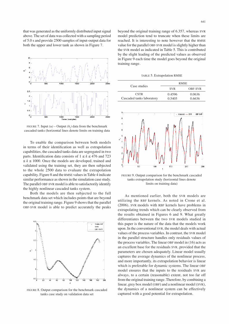
that was generated as the uniformly distributed input signal above. The set of data was collected with a sampling period of 5.0 s and provide 2500 samples of input-output data for both the upper and lower tank as shown in Figure 7.

beyond the original training range of 6.357, whereas SVR model prediction tend to truncate when these limits are reached. It is interesting to note however that the RMSE value for the parallel OBF-SVR model is slightly higher than the SVR model as indicated in Table 5. This is contributed by the slight leading of the predicted values as observed in Figure 9 each time the model goes beyond the original training range.

TABLE 5. Extrapolation RMSE

Case studiesRMSE

SVR OBF-SVR

CSTR Cascaded tanks laboratory

0.45960.5405

0.06360.6636

FIGURE 7. Input (u) – Output (hl) data from the benchmark cascaded tanks (horizontal lines denote limits on training data

To enable the comparison between both models in terms of their identification as well as extrapolation capabilities, the cascaded tanks data are segregated in two parts. Identification data consists of 1 ≤ k ≤ 476 and 723 ≤ k ≤ 1000. Once the models are developed, trained and validated using the training set, they are then subjected to the whole 2500 data to evaluate the extrapolation capability. Figure 8 and the RMSE values in Table 4 indicate similar performance as shown in the simulation case study. The parallel OBF-SVR model is able to satisfactorily identify the highly nonlinear cascaded tanks system. Both the models are then subjected to the full benchmark data set which includes points that are beyond the original training range. Figure 9 shows that the parallel OBF-SVR model is able to predict accurately the peaks

FIGURE 8. Output comparison for the benchmark cascaded tanks case study on validation data set

FIGURE 9. Output comparison for the benchmark cascaded tanks extrapolation study (horizontal lines denote

limits on training data)

As mentioned earlier, both the SVR models are utilizing the RBF kernels. As noted in Crone et al. (2006), SVR models with RBF kernels have problems in extrapolating trends which can be clearly observed from the results obtained in Figures 6 and 9. What greatly differentiates between the two SVR models studied in this paper is the nature of the data that the models work upon. In the conventional SVR, the model deals with actual values of the process variables. In contrast, the SVR model in the parallel structure handles only residuals values of the process variables. The linear OBF model in (16) acts as an excellent base for the residuals SVR, provided that the parameters are chosen adequately. Linear model usually captures the average dynamics of the nonlinear process, and more importantly, its extrapolation behavior is linear which is preferable for dynamic systems. The linear OBF model ensures that the inputs to the residuals SVR are always, to a certain (reasonable) extent, not too far off from the original training range. Therefore, by combining a linear, grey box model (OBF) and a nonlinear model (SVR), the dynamics of a nonlinear system can be effectively captured with a good potential for extrapolation.

642

CONCLUSION

In this paper, parallel OBF-SVR model has been developed as an alternative of support vector machine model. A comparative study has been performed for two different models, namely SVR model and SVR model in parallel with linear OBF (parallel OBF-SVR) model. Identification results show that even though all models are able to identify nonlinear systems efficiently, the proposed parallel OBF-SVR has better performance than SVR model when subjected to out-of-sample test data beyond the original training range with unknown minimum and maximum values. It may be concluded that not all nonlinear models may perform well in range extrapolated regions even though they may be very accurate in the range of training data. Future work is to extend the study for other type of kernel functions as well as for closed-loop conditions using nonlinear model predictive control.

ACKNOWLEDGEMENTS

The authors would like to acknowledge the funding and facilities provided by Universiti Teknologi PETRONAS for this work.

REFERENCES

Babuška, R. & Verbruggen, H. 2003. Neuro-fuzzy methods for nonlinear system identification. Annual Reviews in Control 27(1): 73-85.

Beyhan, S. & Alci, M. 2010. Fuzzy functions based Arx model and new fuzzy basis function models for nonlinear system identification. Applied Soft Computing 10(2): 439-444.

Billings, S.A. & Wei, H.L. 2005. A new class of wavelet networks for nonlinear system identification. IEEE Transactions on Neural Networks 16(4): 862-874.

Castillo, F., Marshall, K., Green, J. & Kordon, A. 2003. A methodology for combining symbolic regression and design of experiments to improve empirical model building. Paper Presented at the Genetic and Evolutionary Computation Conference - GECCO. Springer: Berlin/Heidelberg. pp. 212-212.

Cheng, Y. & Hu, J. 2012. Nonlinear system identification based on Svr with quasi-linear kernel. IEEE International Joint Conference on Neural Networks (IJCNN). pp.1-8.

Cherkassky, V. & Ma, Y. 2004. Practical selection of Svm parameters and noise estimation for Svm regression. Neural Networks 17(1): 113-126.

Crone, S.F., Guajardo, J. & Weber, R. 2006. The impact of preprocessing on support vector regression and neural networks in time series prediction. Proceedings of the International Conference on Data Mining, Last Vegas. pp. 37-44.

Himmelblau, D.M. 2008. Accounts of experiences in the application of artificial neural networks in chemical engineering. Industrial & Engineering Chemistry Research 47(16): 5782-5796.

Iplikci, S. 2010. Support vector machines based neuro-fuzzy control of nonlinear systems. Neurocomputing 73(10): 2097-2107.

Kordon, A.K. 2004. Hybrid intelligent systems for industrial data analysis. International Journal of Intelligent Systems 19(4): 367-383.

Lennox, B., Montague, G.A., Frith, A.M., Gent, C. & Bevan, V. 2001. Industrial application of neural networks - an investigation. Journal of Process Control 11(5): 497-507.

Lin, S., Zhang, S., Qiao, J., Liu, H. & Yu, G. 2008. A parameter choosing method of Svr for time series prediction. In Young Computer Scientists, 2008. ICYCS 2008. The 9th International Conference for IEEE. pp. 130-135.

Liu, Y., Wang, H., Yu, J. & Li, P. 2010. Selective recursive kernel learning for online identification of nonlinear systems with Narx form. Journal of Process Control 20(2): 181-194.

Ljung, L. 2010. Perspectives on system identification. Annual Reviews in Control 34(1): 1-12.

Lu, Z. & Sun, J. 2009. Non-Mercer hybrid kernel for linear programming support vector regression in nonlinear systems identification. Applied Soft Computing 9(1): 94-99.

Lu, Z., Sun, J. & Butts, K.R. 2009. Linear programming support vector regression with wavelet kernel: A new approach to nonlinear dynamical systems identification. Mathematics and Computers in Simulation 79(7): 2051-2063.

Mahmoodi, S., Montazeri, A., Poshtan, J., Jahed-Motlagh, M. & Poshtan, M. 2007. Volterra-Laguerre modeling for Nmpc. In Signal Processsing and Its Applications, 2007, ISSPA 2007, 9th International Symposium on IEEE. pp. 1-4.

Nelles, O. 2013. Nonlinear System Identification: From Classical Approaches to Neural Networks and Fuzzy Models. New York: Springer Science & Business Media.

Nørgård, P.M., Ravn, O., Poulsen, N.K. & Hansen, L.K. 2000. Neural Networks for Modelling and Control of Dynamic Systems-a Practitioner’s Handbook. Location: Publisher.

Ratcliffe, S.J. & Shults, J. 2008. Geeqbox: A Matlab toolbox for generalized estimating equations and quasi-least squares. Journal of Statistical Software 25(14): 1-14.

Shirzad, A., Tabesh, M. & Farmani, R. 2014. A comparison between performance of support vector regression and artificial neural network in prediction of pipe burst rate in water distribution networks. KSCE Journal of Civil Engineering 18(4): 941-948.

Smola, A.J. & Schölkopf, B. 2004. A tutorial on support vector regression. Statistics and Computing 14(3): 199-222.

Suganyadevi, M.V. & Babulal, C.K. 2014. Support vector regression model for the prediction of loadability margin of a power system. Applied Soft Computing 24: 304-315.

Tötterman, S. & Toivonen, H.T. 2009. Support vector method for identification of Wiener models. Journal of Process Control 19(7): 1174-1181.

Tufa, L.D., Ramasamy, M. & Shuhaimi, M. 2011. Improved method for development of parsimonious orthonormal basis filter models. Journal of Process Control 21(1): 36-45.

Wang, X., Dong, J., Hang, Y. & Du, Z. 2013. Identification of nonlinear system via Svr optimized by particle swarm algorithm. Journal of Theoretical & Applied Information Technology 48(2): 967-972.

Wigren, T. 2006. Recursive prediction error identification and scaling of non-linear state space models using a restricted black box parameterization. Automatica 42(1): 159-168.

Wigren, T. & Schoukens, J. 2013. Three free data sets for development and benchmarking in nonlinear system identification. In IEEE Control Conference (ECC), 2013 European. pp. 2933-2938.

Yao, X.J., Panaye, A., Doucet, J.P., Zhang, R.S., Chen, H.F., Liu, M.C., Hu, Z.D. & Fan, B.T. 2004. Comparative study of Qsar/Qspr correlations using support vector machines,

643

radial basis function neural networks, and multiple linear regression. Journal of Chemical Information and Computer Sciences 44(4): 1257-1266.

Zabiri, H., Ramasamy, M., Tufa, L.D. & Maulud, A. 2013. Integrated Obf-Nn models with enhanced extrapolation capability for nonlinear systems. Journal of Process Control 23(10): 1562-1566.

Chemical Engineering DepartmentUniversiti Teknologi PETRONAS32610 Bandar Seri Iskandar, Perak Darul RidzuanMalaysia

*Corresponding author; email: haslindazabiri@utp.edu.my

Received: 7 March 2017Accepted: 26 September 2017