i

OPTIMIZATION OF SHIP ROUTING USING HYBRID GENETIC ALGORITHM

ISMAIL

THESIS SUBMITTED IN FULLFILLMENT OF THE REQUIREMENTS FOR THE DEGREE OF

DOCTOR OF PHILOSOPHY

FACULTY OF COMPUTER SCIENCE AND INFORMATION TECHNOLOGY

UNIVERSITY OF MALAYA KUALA LUMPUR

2014

ii

ABSTRACT

Vehicle Routing Problem (VRP) relates to the problem of providing optimum service with a fleet of vehicles to customers. It is a combinatorial optimization problem. The objective is usually to maximize the profit of the operation. However, for public transportation owned and operated by government, accessibility takes priority over profitability. Accessibility usually reduces profit, while increasing profit tends to reduce accessibility. In this research, we look at how accessibility can be increased without penalizing the profitability. This requires the determination of routes with minimum fuel consumption, maximum number of ports of call and maximum load factor satisfying a number of pre-determined constraints, i.e. hard and soft constraints. The hard constraints are travel time, travel distance and the restriction that a route must contain at least one fuel port. Soft constraints concerns with ship draft and load factor. To solve this problem, we propose a hybrid genetic algorithm (hybrid GA). A chromosome in the proposed hybrid GA consists of some sub-chromosomes and each sub-chromosome consists of Q-arm, P-arm and two centromere. The initial population is generated randomly for the centromere while Q-arm and P-arm are generated by the nearest neighbor. An improvement procedure is proposed to increase the performance of the hybrid GA. The improvement procedure ensures a chromosome with the best fitness is carried forward into the next generation. To evaluate the algorithm, three experiments are carried out. The first experiment is to investigate performance of the hybrid GA algorithm over 11 benchmarks. The results from this experiment show that the hybrid GA has better performance compared to the general GA, the PELNI method and the heuristic algorithm. The second experiment is to generate routes using three algorithms discussed in the research. The results shows that the best routes are generated by the hybrid GA followed by the general GA while the PELNI method shows the worst performance. The best and the worst fitness of the best solution in the second experiment were recorded. It is used to study the performance of the hybrid GA when compared to the general GA. The third experiment is to generate optimum routes when the number of vehicle used is minimized. The result of the experiments show that the hybrid GA performance better than the other algorithms.

iii

ABSTRAK

Masalah perjalanan kendaraan berkaitan dengan masalah dalam menyediakan perkhidmatan yang optimum dengan armada kenderaan kepada pelanggan. Ini merupakan kombinasi masalah pengoptimuman. Objektif yang biasa adalah untuk memaksimumkan keuntungan operasi. Walau bagaimanapun, bagi pengangkutan awam yang dimiliki dan dikendalikan oleh kerajaan, kebolehcapaian merupakan keutamaan berbanding keuntungan. Kebolehcapaian biasanya mengurangkan keuntungan, manakala peningkatan keuntungan cenderung untuk mengurangkan kebolehcapaian. Dalam kajian ini, kita melihat bagaimana kemudahan boleh ditingkatkan tanpa mengurangkan keuntungan. Ini memerlukan penentuan laluan dengan penggunaan bahan api minimum, bilangan maksimum pelabuhan yang dilayani dan faktor beban maksimum yang boleh memenuhi beberapa kekangan yang telah ditetapkan; kekangan keras dan lembut. Kekangan keras meliputi masa perjalanan, jarak perjalanan dan sekatan bahawa laluan mesti mempunyai sekurang-kurangnya satu pelabuhan bahan api. Kekangan lembut pula berkait dengan draf kapal dan faktor muatan. Untuk menyelesaikan masalah ini, kami mencadangkan hybrid genetic algorithm (hybrid GA). Sebuah kromosom dalam hybrid GA terdiri dari sejumlah sub-chromosome dan setiap sub-chromosome terdiri daripada Q-arm, P-arm dan dua centromere. Populasi awal dihasilkan secara rawak untuk centromere manakala Q-arm dan P-arm dihasilkan melalui kaedah nearest neighbor. Satu prosedur penambahbaikan dicadangkan untuk meningkatkan prestasi hybrid GA. Prosedur tersebut memastikan kromosom dengan kecergasan terbaik dibawa ke generasi seterusnya. Untuk menilai algoritma, tiga eksperimen dijalankan. Eksperimen pertama adalah untuk mengkaji algoritma hybrid GA melalui 11 tanda aras. Hasil daripada eksperimen ini menunjukkan bahawa hybrid GA mempunyai prestasi yang lebih baik berbanding dengan general GA, kaedah PELNI dan algoritma heuristik. Eksperimen kedua adalah untuk menjana laluan menggunakan tiga algoritma yang telah dibincangkan dalam penyelidikan. Hasilnya menunjukkan bahawa laluan yang terbaik dihasilkan oleh hybrid GA diikuti oleh general GA manakala kaedah PELNI menunjukkan prestasi terburuk. Eksperimen ketiga ialah untuk menjana laluan optimum apabila jumlah kenderaan yang digunakan adalah minimum. Hasil daripada ekperimen menunjukkan bahwa prestasi hybrid GA adalah lebih baik dibandingkan dengan kaedah lain.

iv

ACKNOWLEDGMENTS

I would like to thank Almighty Allah SWT Most Gracious, Most Merciful.

I would like to express my deepest appreciation to my supervisor, Prof. Dr. Mohd

Sapiyan Baba, for giving me the opportunity to express my ideas via this project,

providing constructive feedbacks, unfailing support and overall help in all aspects of

this work. He contributed too many valuable insights into my research and he also

directed the entire process and the writing of this project. Without his supervision, this

project would not have been possible.

I highly appreciate the efforts of Dr. Effirul Ikhwan Ramlan, Dr. Barnabé Dorronsoro,

Dr. Ayed Atallah Salman, Prof. Kenneth A. De Jong and Dr. Claudia Archetti who

shared their practical experiences and ideas. Thanks are also extended to all of my

friends in Artificial Intelligence Laboratory for their input and cooperation during my

study.

For financial support, I gratefully acknowledge University of Malaya.

v

DEDICATION

To my beloved:

Mother, Hjh. Siti Rahmah

Mother in Law, Pn. Rokiah bte Ahmad

Father, Hj. Drs. Muh. Yusuf

Wife, Rohana bte Abd. Hakim

Daughters, Andi Almeira Zocha and Andi Regina Acacia

vi

TABLE OF CONTENTS

ABSTRACT .................................................................................................. ii

ABSTRAK ..................................................................................................... iii

ACKNOWLEDGMENTS ............................................................................. iv

DEDICATION .............................................................................................. v

TABLE OF CONTENTS .............................................................................. vi

LIST OF FIGURES ....................................................................................... x

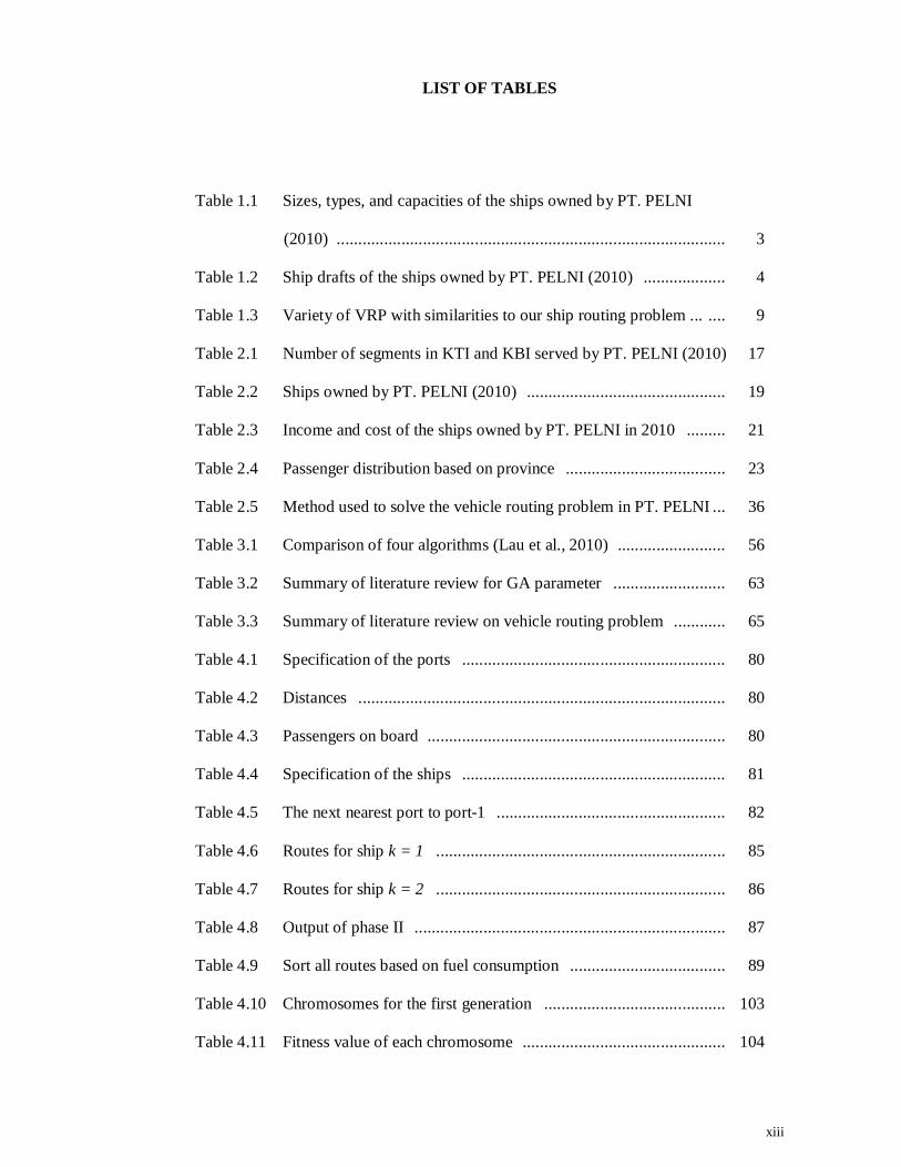
LIST OF TABLES ........................................................................................ xiii

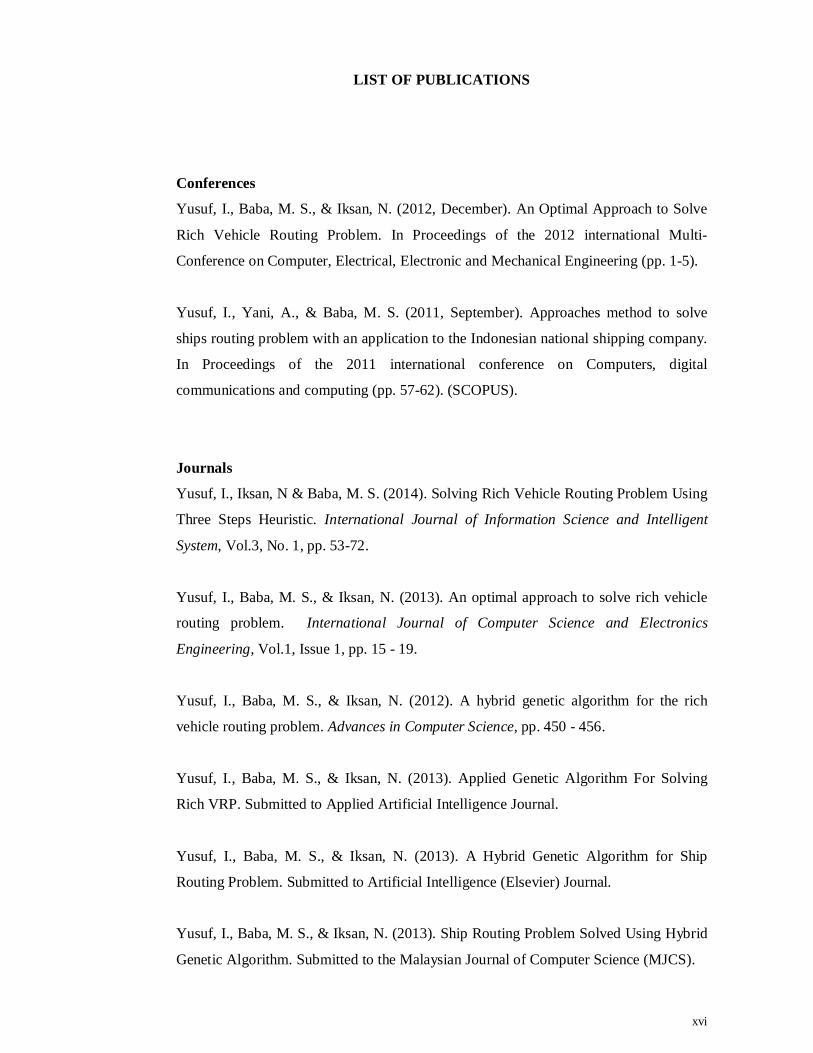
LIST OF PUBLICATIONS ........................................................................... xvi

LIST OF NOTATIONS ................................................................................ xvii

Chapter 1 INTRODUCTION .................................................................... 1

1.1 Problem Statement ............................................................................... 2

1.2 Aims and Objectives ............................................................................ 6

1.3 Research Methodology ........................................................................ 8

1.4 Thesis Layout ...................................................................................... 10

Chapter 2 SHIP ROUTING PROBLEM IN INDONESIA ...................... 11

2.1 Port ....................................................................................................... 15

2.2 Ship ...................................................................................................... 18

2.3 Passenger .............................................................................................. 22

2.4 Earlier Research about the Routing Problem in PT. PELNI .................... 30

2.5 Summary ............................................................................................... 35

vii

Chapter 3 VEHICLE ROUTING PROBLEM ......................................... 37

3.1 Multi Depot Vehicle Routing Problem ................................................. 39

3.2 Heterogeneous Fleet Vehicle Routing Problem ................................... 40

3.3 Site Dependent Capacitated Vehicle Routing Problem ........................ 42

3.4 Asymmetric Vehicle Routing Problem ................................................. 43

3.5 Solution to the VRP ............................................................................. 43

3.5.1 Heuristic for VRP ..................................................................... 44

3.5.1.1 Route Construction ................................................... 45

3.5.1.2 Two Phase (Clustering and Routing) Method ........... 46

3.5.1.3 Route Improvement .................................................. 48

3.5.2 Metaheuristic for VRP .............................................................. 48

3.6 Genetic Algorithm ............................................................................... 53

3.7 Summary ............................................................................................. 64

Chapter 4 DEVELOPMENT OF ALGORITHM FOR SHIP ROUTING . 66

4.1 Ship Routing Problem Model ............................................................... 67

4.1.1 Objective .................................................................................. 67

4.1.2 Constraints ............................................................................... 68

4.1.3 Mathematical Model ................................................................. 72

4.2 Heuristic Method ................................................................................. 75

4.2.1 Heuristic for Ship Routing Problem ......................................... 76

4.2.2 Illustration of Heuristic ............................................................. 79

4.3 Genetic Algorithm ............................................................................... 91

4.3.1 Genetic Algorithm for Ship Routing Problem .......................... 91

4.3.2 Illustration of General Genetic Algorithm ................................ 98

4.4 Hybrid Genetic Algorithm for Ship Routing Problem ......................... 118

4.5 Summary ............................................................................................. 121

viii

Chapter 5 RESULT AND ANALYSIS ......................................................... 123

5.1 Experiment 1 - Performance of Three Algorithms Compared with

Prior Work ............................................................................................ 123

5.1.1 The Benchmarks Problem ......................................................... 123

5.1.2 Result ........................................................................................ 136

5.1.3 Analysis .................................................................................... 141

5.1.4 Comparing the Performances of PELNI Method, Heuristic

Algorithm, General Genetic Algorithm and Hybrid Genetic

Algorithm .................................................................................. 147

5.2 Experiment 2 - Implementation of Algorithm ....................................... 148

5.2.1 Existing Routes in PT. PELNI 2010 .......................................... 148

5.2.2 Routes Generated Using a General Genetic Algorithm .............. 152

5.2.3 Routes Generated Using a Hybrid Genetic Algorithm ................ 156

5.2.4 Analysis .................................................................................... 160

5.3 Experiment 3 - Routes Proposed ........................................................... 166

5.4 Summary .............................................................................................. 171

Chapter 6 CONCLUSIONS AND FUTURE WORK .................................. 173

6.1 Research Summary ............................................................................... 173

6.2 Contribution .......................................................................................... 177

6.3 Limitation ............................................................................................. 179

6.4 Further Work ........................................................................................ 180

6.5 Conclusion ............................................................................................ 180

BIBLIOGRAPHY .......................................................................................... 181

ix

Appendix ........................................................................................................ 189

Appendix A - Ports and Routes ..................................................................... 190

Appendix B - Benchmarks ............................................................................. 219

Appendix C - Routes ...................................................................................... 223

Appendix D - Comparison of Four Algorithms .............................................. 232

x

LIST OF FIGURES

Figure 2.1 Pattern of the relationships in transportation system .................. 11

Figure 2.2 Indonesia archipelago ................................................................ 14

Figure 2.3 National shipping networks served by PT. PELNI in 2010 ........ 16

Figure 2.4 Operational cost of PT. PELNI in 2010 ..................................... 20

Figure 2.5 Characteristics of PT. PELNI passengers; based on gender ........ 24

Figure 2.6 Characteristics of PT. PELNI passengers; based on age ............. 25

Figure 2.7 Characteristics of PT. PELNI passengers; based on marital status 25

Figure 2.8 Characteristic of PT. PELNI passengers; based on the occupation 26

Figure 2.9 Characteristics of PT. PELNI passengers; based on education ... 27

Figure 2.10 Characteristics of PT. PELNI passengers; based on salary ......... 27

Figure 2.11 Main purpose of journey (2010) ................................................ 28

Figure 2.12 Frequently travelled between islands (2010) .............................. 28

Figure 2.13 Reasons to use PT. PELNI services (2010) ................................ 29

Figure 2.14 Rely on the services of PT. PELNI (2010) ................................. 29

Figure 2.15 Generating routes in Pertiwi (2005) ........................................... 33

Figure 2.16 Choosing the best routes in Pertiwi (2005) ................................ 34

Figure 3.1 Method used for VRP ................................................................ 44

Figure 3.2 Genetic Algorithm; generate chromosomes, evaluate the

fitness value, selection and recombination ................................. 54

Figure 3.3 Chromosome encoding method ................................................. 57

Figure 3.4 Single point crossover: One offspring consists of the gene from

one parent into the left of the point, and from the other parent

to the right of the point .............................................................. 61

xi

Figure 4.1 Research framework .................................................................. 66

Figure 4.2 Clustering .................................................................................. 77

Figure 4.3 Assigning vehicle ...................................................................... 78

Figure 4.4 Finding best routes .................................................................... 79

Figure 4.5 Steps for finding the next nearest port ........................................ 84

Figure 4.6 Genetic Algorithm for vehicle routing problem ......................... 92

Figure 4.7 Q-arm and P-arm in chromosome proposed ............................... 93

Figure 4.8 Representation of the chromosome for two ships ....................... 93

Figure 4.9 Multi Cut Point Crossover ......................................................... 96

Figure 4.10 Pairs Exchange Mutation ........................................................... 97

Figure 4.11 Chromosome: 2 ships, 4 customer ports and 2 fuel ports ............ 99

Figure 4.12 Generated chromosomes ........................................................... 99

Figure 4.13 Crossover for s’1 vs. s’8 ............................................................. 110

Figure 4.14 Pairs exchange mutation ............................................................ 114

Figure 4.15 Repairing chromosomes ............................................................ 115

Figure 4.16 Hybrid Genetic Algorithm proposed .......................................... 118

Figure 4.17 Chromosomes for initial population using the hybrid Genetic

Algorithm .................................................................................. 120

Figure 5.1 Routes of the benchmark; 40c-9d-8k ......................................... 125

Figure 5.2 Routes of the benchmark; 28c-9d-9k ......................................... 126

Figure 5.3 Routes of the benchmark; 45c-11d-11k ..................................... 127

Figure 5.4 Routes of the benchmark; 32c-4d-8k ......................................... 128

Figure 5.5 Routes of the benchmark; 34c-11d-11k ..................................... 129

Figure 5.6 Routes of the benchmark; 63c-14d-11k ..................................... 130

Figure 5.7 Routes of the benchmark; 18c-6d-8k ......................................... 131

Figure 5.8 Routes of the benchmark; 28c-6d-11k ....................................... 132

xii

Figure 5.9 Routes of the benchmark; 12c-4d-8k ......................................... 133

Figure 5.10 Routes of the benchmark; 53c-12d-11k ..................................... 134

Figure 5.11 Routes of the benchmark; 24c-5d-10k ....................................... 135

Figure 5.12 Performance of four algorithms in terms of fuel consumption...... 143

Figure 5.13 Performance of four algorithms in terms the number of ports

of call ........................................................................................ 145

Figure 5.14 Performance of four algorithms in terms of the load factor ........ 147

Figure 5.15 Routes generated by PELNI method (PELNI, 2010) .................. 151

Figure 5.16 Routes generated by general Genetic Algorithm ........................ 155

Figure 5.17 Routes generated by hybrid Genetic Algorithm ......................... 159

Figure 5.18 Performance of three algorithms in terms the fuel consumption ... 160

Figure 5.19 Performance of three algorithms in terms the number of ports

of call ........................................................................................ 161

Figure 5.20 Performance of three algorithms in terms the load factor ........... 162

Figure 5.21 Quadrant scale of PELNI method (PELNI, 2010) ...................... 163

Figure 5.22 Quadrant scale of general Genetic Algorithm ............................ 164

Figure 5.23 Quadrant scale of hybrid Genetic Algorithm .............................. 165

Figure 5.24 Routes proposed for minimum ships scenarios that generated

by hybrid Genetic Algorithm ..................................................... 169

Figure 5.25 Quadrant scale for minimum ships scenarios ............................. 170

xiii

LIST OF TABLES

Table 1.1 Sizes, types, and capacities of the ships owned by PT. PELNI

(2010) .......................................................................................... 3

Table 1.2 Ship drafts of the ships owned by PT. PELNI (2010) ................... 4

Table 1.3 Variety of VRP with similarities to our ship routing problem ... .... 9

Table 2.1 Number of segments in KTI and KBI served by PT. PELNI (2010) 17

Table 2.2 Ships owned by PT. PELNI (2010) .............................................. 19

Table 2.3 Income and cost of the ships owned by PT. PELNI in 2010 ......... 21

Table 2.4 Passenger distribution based on province ..................................... 23

Table 2.5 Method used to solve the vehicle routing problem in PT. PELNI ... 36

Table 3.1 Comparison of four algorithms (Lau et al., 2010) ......................... 56

Table 3.2 Summary of literature review for GA parameter .......................... 63

Table 3.3 Summary of literature review on vehicle routing problem ............ 65

Table 4.1 Specification of the ports ............................................................. 80

Table 4.2 Distances ..................................................................................... 80

Table 4.3 Passengers on board ..................................................................... 80

Table 4.4 Specification of the ships ............................................................. 81

Table 4.5 The next nearest port to port-1 ..................................................... 82

Table 4.6 Routes for ship k = 1 ................................................................... 85

Table 4.7 Routes for ship k = 2 ................................................................... 86

Table 4.8 Output of phase II ........................................................................ 87

Table 4.9 Sort all routes based on fuel consumption .................................... 89

Table 4.10 Chromosomes for the first generation .......................................... 103

Table 4.11 Fitness value of each chromosome ............................................... 104

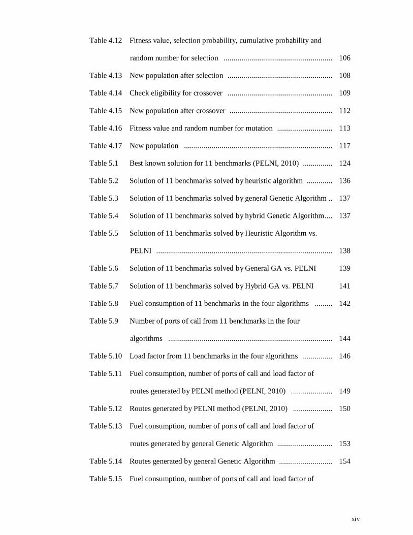
xiv

Table 4.12 Fitness value, selection probability, cumulative probability and

random number for selection ....................................................... 106

Table 4.13 New population after selection ..................................................... 108

Table 4.14 Check eligibility for crossover ..................................................... 109

Table 4.15 New population after crossover .................................................... 112

Table 4.16 Fitness value and random number for mutation ............................ 113

Table 4.17 New population ........................................................................... 117

Table 5.1 Best known solution for 11 benchmarks (PELNI, 2010) ............... 124

Table 5.2 Solution of 11 benchmarks solved by heuristic algorithm ............. 136

Table 5.3 Solution of 11 benchmarks solved by general Genetic Algorithm .. 137

Table 5.4 Solution of 11 benchmarks solved by hybrid Genetic Algorithm .... 137

Table 5.5 Solution of 11 benchmarks solved by Heuristic Algorithm vs.

PELNI ......................................................................................... 138

Table 5.6 Solution of 11 benchmarks solved by General GA vs. PELNI ...... 139

Table 5.7 Solution of 11 benchmarks solved by Hybrid GA vs. PELNI ....... 141

Table 5.8 Fuel consumption of 11 benchmarks in the four algorithms ......... 142

Table 5.9 Number of ports of call from 11 benchmarks in the four

algorithms ................................................................................... 144

Table 5.10 Load factor from 11 benchmarks in the four algorithms ............... 146

Table 5.11 Fuel consumption, number of ports of call and load factor of

routes generated by PELNI method (PELNI, 2010) ..................... 149

Table 5.12 Routes generated by PELNI method (PELNI, 2010) .................... 150

Table 5.13 Fuel consumption, number of ports of call and load factor of

routes generated by general Genetic Algorithm ............................ 153

Table 5.14 Routes generated by general Genetic Algorithm ........................... 154

Table 5.15 Fuel consumption, number of ports of call and load factor of

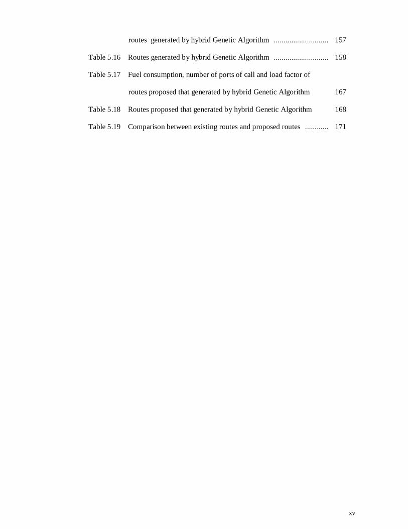
xv

routes generated by hybrid Genetic Algorithm ............................ 157

Table 5.16 Routes generated by hybrid Genetic Algorithm ............................ 158

Table 5.17 Fuel consumption, number of ports of call and load factor of

routes proposed that generated by hybrid Genetic Algorithm ....... 167

Table 5.18 Routes proposed that generated by hybrid Genetic Algorithm ........ 168

Table 5.19 Comparison between existing routes and proposed routes ............ 171

xvi

LIST OF PUBLICATIONS

Conferences

Yusuf, I., Baba, M. S., & Iksan, N. (2012, December). An Optimal Approach to Solve

Rich Vehicle Routing Problem. In Proceedings of the 2012 international Multi-

Conference on Computer, Electrical, Electronic and Mechanical Engineering (pp. 1-5).

Yusuf, I., Yani, A., & Baba, M. S. (2011, September). Approaches method to solve

ships routing problem with an application to the Indonesian national shipping company.

In Proceedings of the 2011 international conference on Computers, digital

communications and computing (pp. 57-62). (SCOPUS).

Journals

Yusuf, I., Iksan, N & Baba, M. S. (2014). Solving Rich Vehicle Routing Problem Using

Three Steps Heuristic. International Journal of Information Science and Intelligent

System, Vol.3, No. 1, pp. 53-72.

Yusuf, I., Baba, M. S., & Iksan, N. (2013). An optimal approach to solve rich vehicle

routing problem. International Journal of Computer Science and Electronics

Engineering, Vol.1, Issue 1, pp. 15 - 19.

Yusuf, I., Baba, M. S., & Iksan, N. (2012). A hybrid genetic algorithm for the rich

vehicle routing problem. Advances in Computer Science, pp. 450 - 456.

Yusuf, I., Baba, M. S., & Iksan, N. (2013). Applied Genetic Algorithm For Solving

Rich VRP. Submitted to Applied Artificial Intelligence Journal.

Yusuf, I., Baba, M. S., & Iksan, N. (2013). A Hybrid Genetic Algorithm for Ship

Routing Problem. Submitted to Artificial Intelligence (Elsevier) Journal.

Yusuf, I., Baba, M. S., & Iksan, N. (2013). Ship Routing Problem Solved Using Hybrid

Genetic Algorithm. Submitted to the Malaysian Journal of Computer Science (MJCS).

xvii

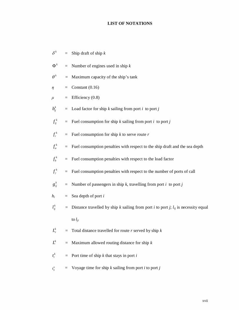
LIST OF NOTATIONS

k = Ship draft of ship k

k = Number of engines used in ship k

k = Maximum capacity of the ship’s tank

η = Constant (0.16)

μ = Efficiency (0.8)

kijb = Load factor for ship k sailing from port i to port j

kijf = Fuel consumption for ship k sailing from port i to port j

krf = Fuel consumption for ship k to serve route r

kf = Fuel consumption penalties with respect to the ship draft and the sea depth

kbf = Fuel consumption penalties with respect to the load factor

kf = Fuel consumption penalties with respect to the number of ports of call

kijg = Number of passengers in ship k, travelling from port i to port j

hi = Sea depth of port i

kijl = Distance travelled by ship k sailing from port i to port j; lij is necessity equal

to lji

krL = Total distance travelled for route r served by ship k

kL = Maximum allowed routing distance for ship k

kit = Port time of ship k that stays in port i

kijt = Voyage time for ship k sailing from port i to port j

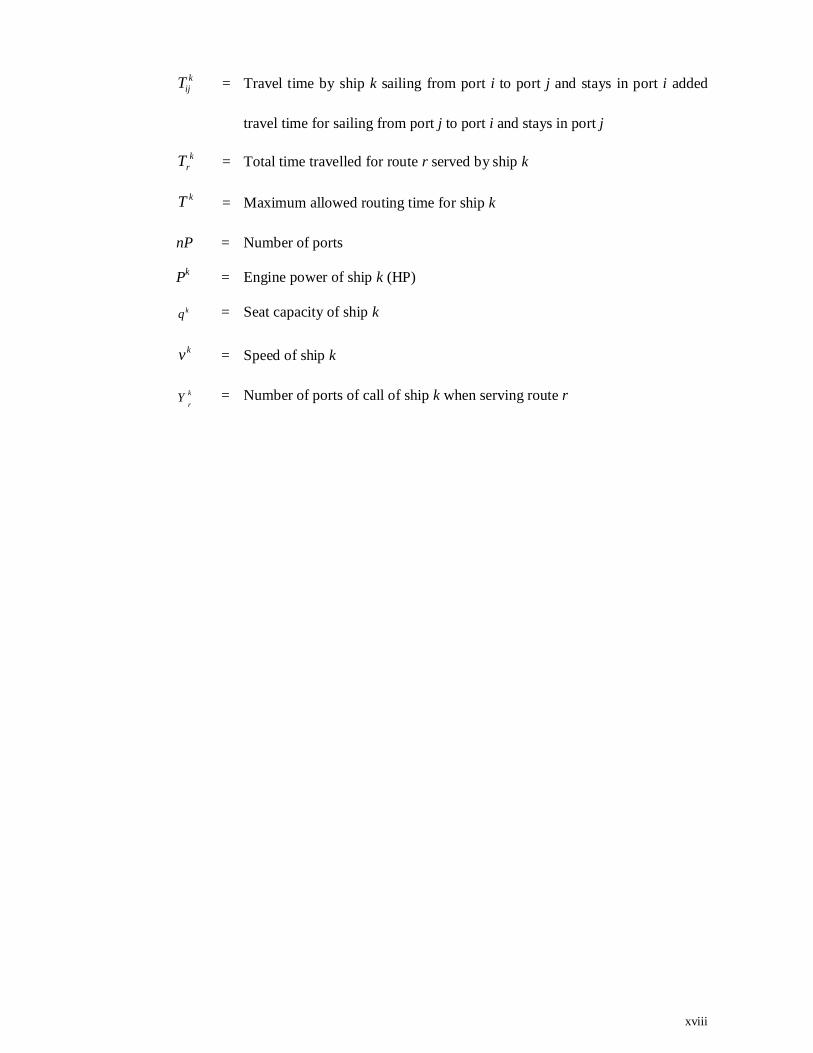
xviii

kijT = Travel time by ship k sailing from port i to port j and stays in port i added

travel time for sailing from port j to port i and stays in port j

krT = Total time travelled for route r served by ship k

kT = Maximum allowed routing time for ship k

nP = Number of ports

Pk = Engine power of ship k (HP)

kq = Seat capacity of ship k

kv = Speed of ship k

kr

Y = Number of ports of call of ship k when serving route r

1

CHAPTER 1 INTRODUCTION

Transportation is fundamental to the development of a nation’s industry and economy

(Japan International Corporation Agency, 2004). Transportation problems are complex

and involve solving multiple objectives at the same time. Many research groups

worldwide have studied transportation problems; and have often simplified the issues

using real world cases. The effectiveness of transportation systems depends on the

suitability of routes for the various types of vehicles available. Related studies are

known as vehicle routing problems (Pertiwi, 2005).

Vehicle routing problems, which are some of the most important studies in the fields of

transportation, involves routes that are designed for the benefit of passengers and

operators, employing optimal routes to meet the objectives and interests of both parties.

Problems often faced by transportation service providers include limited allocation of

resources (e.g. financial and infrastructure). Determining optimal routes must take into

account the allocation of resources for an efficient transport service (Japan International

Corporation Agency, 2004).

The vehicle routing problem is a combination of optimization processes seeking to

service a number of customers with a number of vehicles. As a generic name, it is given

to a whole class of problems in which a set of routes, for a fleet of vehicles based at one

or more depots must be determined for geographically dispersed cities and customers

(Cordeau et. al., 1997).

2

There are many variations that depend on the characteristics of the vehicles, customers,

and facilities (Cordeau et. al., 1997). For example, the vehicles may be either identical

or different (with respect to size); they may be restricted to serve each customer

depending on their suitability and the customers; and the problem may involve a single

facility or multiple facilities. Many cases require a combination of two or more of these

variants in order to solve a real world problem.

1.1 Problem Statement

In public transportation owned and operated by the government the most important

factors to consider are accessibility and profitability. Accessibility consists of how to

maximise the number of ports of call and profitability consists of how to minimise fuel

consumption whilst maximising the load factor by satisfying a number of predetermined

constraints (PELNI, 2010).

Accessibility usually reduces profit; an increasing profit tends to reduce accessibility. To

increase profit, fuel consumption may have to be reduced, but this may affect the

number of ports of call. However, increasing profits by decreasing the number of ports

of call will decrease accessibility. The goal of increasing profit can conflict with the aim

of increasing accessibility. To overcome these problems, an operational strategy is

required to minimise conflicts of interest between accessibility and profitability.

In this research, PELNI’s routing was chosen as the case study. PELNI is a

transportation company owned and operated by the Indonesian government. PELNI lost

Rp . 1,427,610,866,209 in 2007 and Rp. 1,561,235,420,278 in 2008 (PELNI, 2008).

3

A way to reduce losses in existing available resources (i.e., ships and their crews) is the

optimization of routes. There are two important things to consider in the optimum routes

of our case study; namely accessibility and profitability. In this research, we used

computational intelligence to help create a route that met both of these conditions.

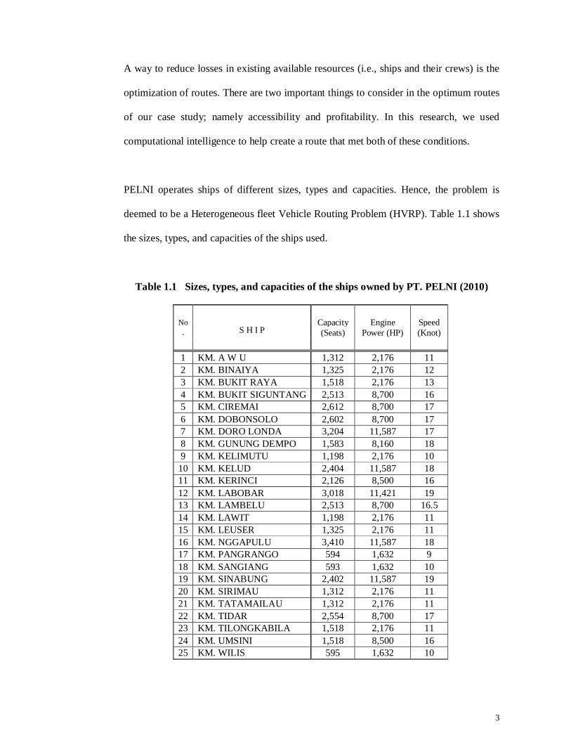
PELNI operates ships of different sizes, types and capacities. Hence, the problem is

deemed to be a Heterogeneous fleet Vehicle Routing Problem (HVRP). Table 1.1 shows

the sizes, types, and capacities of the ships used.

Table 1.1 Sizes, types, and capacities of the ships owned by PT. PELNI (2010)

No.

Capacity (Seats)

Engine Power (HP)

Speed (Knot) S H I P

1 KM. A W U 1,312 2,176 11 2 KM. BINAIYA 1,325 2,176 12 3 KM. BUKIT RAYA 1,518 2,176 13 4 KM. BUKIT SIGUNTANG 2,513 8,700 16 5 KM. CIREMAI 2,612 8,700 17 6 KM. DOBONSOLO 2,602 8,700 17 7 KM. DORO LONDA 3,204 11,587 17 8 KM. GUNUNG DEMPO 1,583 8,160 18 9 KM. KELIMUTU 1,198 2,176 10

10 KM. KELUD 2,404 11,587 18 11 KM. KERINCI 2,126 8,500 16 12 KM. LABOBAR 3,018 11,421 19 13 KM. LAMBELU 2,513 8,700 16.5 14 KM. LAWIT 1,198 2,176 11 15 KM. LEUSER 1,325 2,176 11 16 KM. NGGAPULU 3,410 11,587 18 17 KM. PANGRANGO 594 1,632 9 18 KM. SANGIANG 593 1,632 10 19 KM. SINABUNG 2,402 11,587 19 20 KM. SIRIMAU 1,312 2,176 11 21 KM. TATAMAILAU 1,312 2,176 11 22 KM. TIDAR 2,554 8,700 17 23 KM. TILONGKABILA 1,518 2,176 11 24 KM. UMSINI 1,518 8,500 16 25 KM. WILIS 595 1,632 10

4

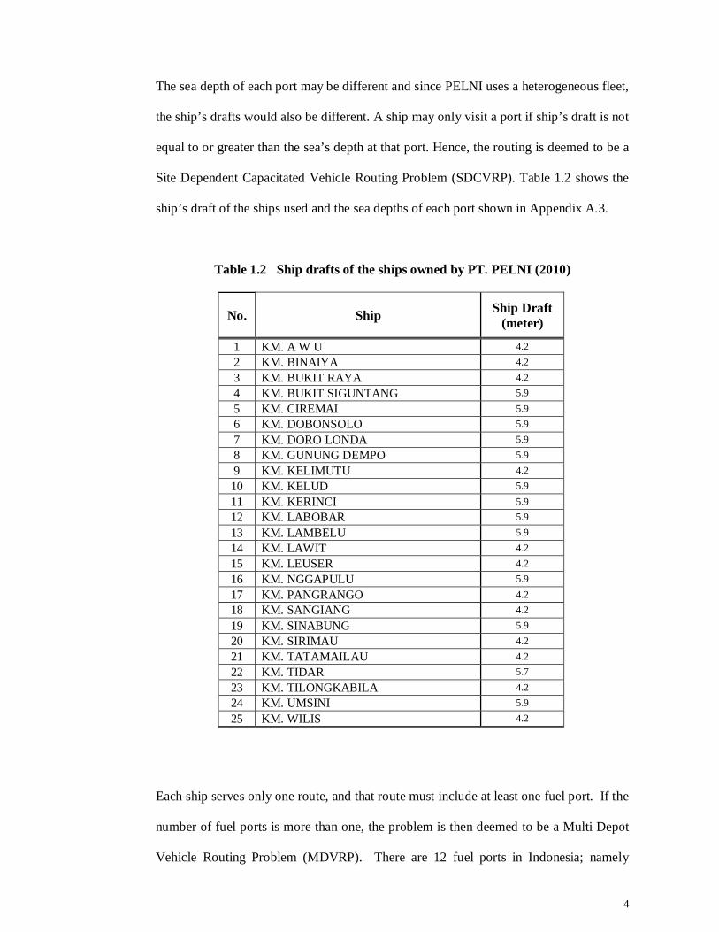
The sea depth of each port may be different and since PELNI uses a heterogeneous fleet,

the ship’s drafts would also be different. A ship may only visit a port if ship’s draft is not

equal to or greater than the sea’s depth at that port. Hence, the routing is deemed to be a

Site Dependent Capacitated Vehicle Routing Problem (SDCVRP). Table 1.2 shows the

ship’s draft of the ships used and the sea depths of each port shown in Appendix A.3.

Table 1.2 Ship drafts of the ships owned by PT. PELNI (2010)

No. Ship Ship Draft (meter)

1 KM. A W U 4.2 2 KM. BINAIYA 4.2 3 KM. BUKIT RAYA 4.2 4 KM. BUKIT SIGUNTANG 5.9

5 KM. CIREMAI 5.9 6 KM. DOBONSOLO 5.9

7 KM. DORO LONDA 5.9 8 KM. GUNUNG DEMPO 5.9 9 KM. KELIMUTU 4.2 10 KM. KELUD 5.9

11 KM. KERINCI 5.9 12 KM. LABOBAR 5.9

13 KM. LAMBELU 5.9 14 KM. LAWIT 4.2 15 KM. LEUSER 4.2 16 KM. NGGAPULU 5.9

17 KM. PANGRANGO 4.2 18 KM. SANGIANG 4.2

19 KM. SINABUNG 5.9 20 KM. SIRIMAU 4.2 21 KM. TATAMAILAU 4.2 22 KM. TIDAR 5.7

23 KM. TILONGKABILA 4.2 24 KM. UMSINI 5.9

25 KM. WILIS 4.2

Each ship serves only one route, and that route must include at least one fuel port. If the

number of fuel ports is more than one, the problem is then deemed to be a Multi Depot

Vehicle Routing Problem (MDVRP). There are 12 fuel ports in Indonesia; namely

5

Ambon, Balikpapan, Belawan, Benoa, Bitung, Kupang, Makassar, Pontianak, Semarang,

Surabaya, Tanjung Priok and Ternate (PELNI, 2010).

The distance travelled from port i to port j may not be the same as that of port j to port i.

This results in an Asymmetric Vehicle Routing Problem (AVRP). The distances between

two ports are shown in Appendix A.4.

By satisfying a number of predetermined constraints, we propose to determine a

combination of routes that will have minimum fuel consumption, maximum number of

ports of call, and maximum load factor. These constraints consist of two soft constraints

and three hard constraints. The soft constraints are ship draft and load factor, and the

hard constraints are travel time, travel distance, and that a route must include at least one

fuel port.

A vehicle has to deliver to n different ports, and then have n! possible route solutions. If

the number of ports is 10 then we have 3,628,800 possible route solutions and if the

number of ships is 10 then we have 36,288,000 possible route solutions for a single

objective. To demonstrate how difficult this problem can be; imagine that the number of

ports is 65, and the number of ships is 25 with three objectives.

This research proposes the use of a population search algorithm (Liu et al., 2004) to

solve the problem. Such algorithms operate on several generations of solution

populations and are able to generate several solutions together in a single iteration. The

population search algorithm is a branch of the meta-heuristic method and can be applied

to multi-objective optimisation problems (Liu et al., 2004).

6

1.2 Aims and Objectives

This research aims to develop an algorithm that will find the optimal route for four

different variants of vehicle routing problems i.e., the Heterogeneous fleet Vehicle

Routing Problem (HVRP), Site Dependent Capacitated Vehicle Routing Problem

(SDCVRP), Multi Depot Vehicle Routing Problem (MDVRP), and Asymmetric Vehicle

Routing Problem (AVRP) with multiple goals. This problem arises from the real

situation faced by PT. PELNI (an Indonesian state-owned ship company). Two

important factors of this state-owned ship company are accessibility and profitability.

The proposed algorithm is meant to:

1. Maximise the number of ports of call

2. Maximise the number of load factor

3. Minimise fuel consumption.

The objectives of this research are as follows:

i. Objective 1: To investigate a variety of vehicle routing problems with

similarities to the ship routing problem in our case study.

The vehicle routing problem has many variations that depend on the characteristics

of the vehicles, the customers, and the facilities. In many cases, a combination of

two or more of these variants for solving a real world problem was needed.

Therefore, we need determine the variant of the vehicle routing problem that has

similarities with the ship routing problem in our case study.

ii. Objective 2: To identify the objective function and constraints of the ship

routing problem in our case study.

In our case study, the two important factors to consider in the ship routing problem

in our case study are accessibility and profitability. Accessibility and profitability

will be used to analyse the performance of the routes. Therefore, we need to

7

determine which suitable objective function can be used to analyse the

performance of the routes in our case study.

Since the ships in PT. PELNI are of different sizes, this may restrict these vehicles

from serving each port; depending on their suitability to the port. This will lead to

both soft and hard constraints. Therefore, we need to determine the soft and hard

constraints in our case study’s ship routing problem.

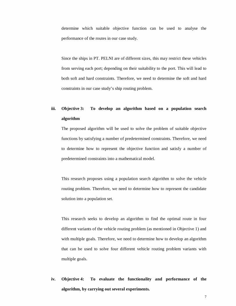
iii. Objective 3: To develop an algorithm based on a population search

algorithm

The proposed algorithm will be used to solve the problem of suitable objective

functions by satisfying a number of predetermined constraints. Therefore, we need

to determine how to represent the objective function and satisfy a number of

predetermined constraints into a mathematical model.

This research proposes using a population search algorithm to solve the vehicle

routing problem. Therefore, we need to determine how to represent the candidate

solution into a population set.

This research seeks to develop an algorithm to find the optimal route in four

different variants of the vehicle routing problem (as mentioned in Objective 1) and

with multiple goals. Therefore, we need to determine how to develop an algorithm

that can be used to solve four different vehicle routing problem variants with

multiple goals.

iv. Objective 4: To evaluate the functionality and performance of the

algorithm, by carrying out several experiments.

8

The Performances of the algorithm proposed in Objective 3 can be evaluated by:

Comparing the proposed algorithm with algorithms presented by other

researchers.

Comparing the routes generated by the proposed algorithm with the existing

case study route.

1.3 Research Methodology

This research was carried out using the following four phases.

Phase 1 - Identifying the problem.

To give a deeper understanding of the ship routing problem, we reviewed literature

by collecting information on other vehicle routing problems and identifying the

relevant issues of ship routing in our case study. A study was conducted to

investigate the performance measurement tools of ship routing and identify their

efficiency in the existing route. Data about ships, passengers, and ports used was

collected for the existing route.

Phase 2 - Mathematical representation of the problem.

To represent the problem in a mathematical form, we determined the objective

function and constraints of the problem. We studied the variety of vehicle routing

problems that were similar to the ship routing in our case study. We summarized

our findings in Table 1.3.

The overall problem consists of minimising fuel consumption, maximizing the

number of ports of call, and the load factor. Meanwhile, the constraints relates to

the ship’s draft, load factor, travel time, travel distance, and inclusion of at least

one fuel port for each route.

9

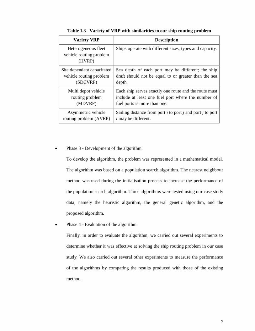
Table 1.3 Variety of VRP with similarities to our ship routing problem

Variety VRP Description

Heterogeneous fleet vehicle routing problem

(HVRP)

Ships operate with different sizes, types and capacity.

Site dependent capacitated vehicle routing problem

(SDCVRP)

Sea depth of each port may be different; the ship draft should not be equal to or greater than the sea depth.

Multi depot vehicle routing problem

(MDVRP)

Each ship serves exactly one route and the route must include at least one fuel port where the number of fuel ports is more than one.

Asymmetric vehicle routing problem (AVRP)

Sailing distance from port i to port j and port j to port i may be different.

Phase 3 - Development of the algorithm

To develop the algorithm, the problem was represented in a mathematical model.

The algorithm was based on a population search algorithm. The nearest neighbour

method was used during the initialisation process to increase the performance of

the population search algorithm. Three algorithms were tested using our case study

data; namely the heuristic algorithm, the general genetic algorithm, and the

proposed algorithm.

Phase 4 - Evaluation of the algorithm

Finally, in order to evaluate the algorithm, we carried out several experiments to

determine whether it was effective at solving the ship routing problem in our case

study. We also carried out several other experiments to measure the performance

of the algorithms by comparing the results produced with those of the existing

method.

10

1.4 Thesis Layout

This thesis contains six chapters. In this chapter, we begun by defining the problem

statement, highlighting the importance of the vehicle routing problem, explaining the

aims and objectives of this thesis, and briefly describing the research methodology.

Chapter 2 is a literature review of the ship routing problem used in our case study. Three

aspects of ship transportation are described i.e., ports, vehicles used and the

passengers/cargo being transported. The survey which was conducted on passenger ships

in our case study is also presented.

In Chapter 3, the literature review of the vehicle routing problem variants associated

with the ship routing problem in our case study are investigated. Algorithms used in

earlier researches for solving vehicle routing problems are discussed.

Chapter 4 describes the development of the heuristics algorithm, the general genetic

algorithm, and the proposed algorithm. Meanwhile, Chapter 5 presents the results of our

experiments. Data from different algorithms were compared and a discussion on the

experimental result is also presented in this chapter.

Finally, Chapter 6 presents the conclusions of the present research and suggests possible

directions for future research.

11

CHAPTER 2 SHIP ROUTING PROBLEM IN INDONESIA

Transportation can be defined as the movement of people or goods for a particular

purpose from one location to another using a transfer mode together with the appropriate

infrastructure. Efficient transportation affects individuals, communities and economies

and it could increase the rate of growth of a community (Christiansen et al., 2005).

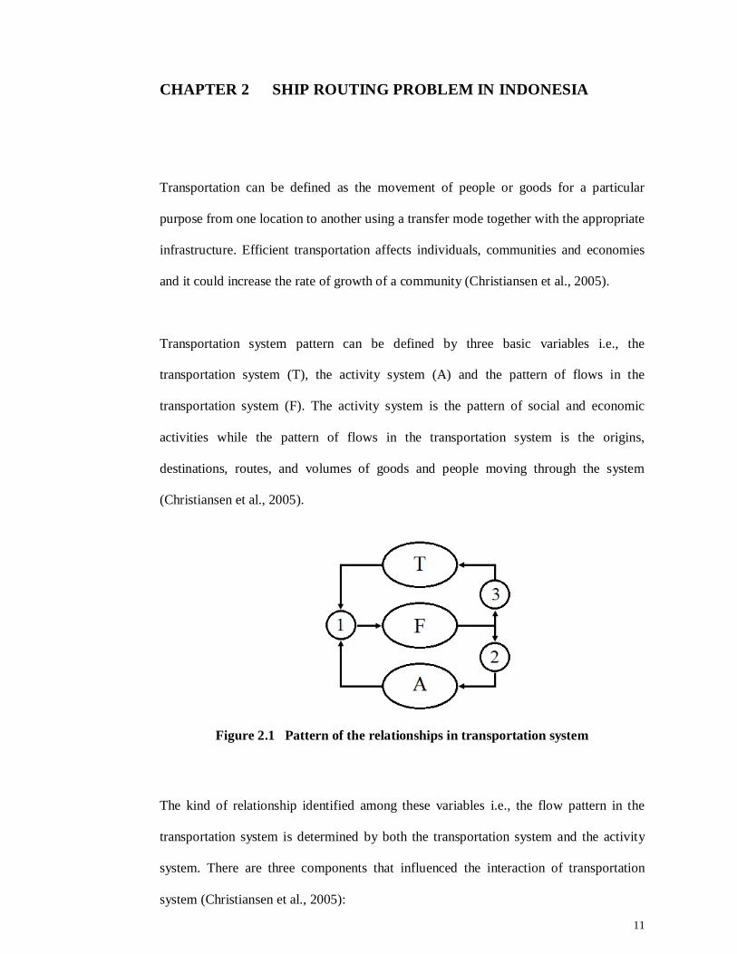
Transportation system pattern can be defined by three basic variables i.e., the

transportation system (T), the activity system (A) and the pattern of flows in the

transportation system (F). The activity system is the pattern of social and economic

activities while the pattern of flows in the transportation system is the origins,

destinations, routes, and volumes of goods and people moving through the system

(Christiansen et al., 2005).

Figure 2.1 Pattern of the relationships in transportation system

The kind of relationship identified among these variables i.e., the flow pattern in the

transportation system is determined by both the transportation system and the activity

system. There are three components that influenced the interaction of transportation

system (Christiansen et al., 2005):

12

1) User (individuals), whether a shipper of goods or a passenger, makes decisions

about when, where, how, and whether to travel.

2) Operator (groups), the operator of particular transportation facilities or services

makes decisions about vehicle routes and schedules, prices to be charged and

services offered, the kinds and quantities of vehicles to be included in the fleet,

the physical facilities to be provided.

3) Regulator (government/institutions), makes decisions on taxes, subsidies, and

other financial matters that influence users and operators; on the provision of

new or improved facilities, and on legal and administrative devices to influence,

encourage, or constrain the decisions of operators or users.

One of the problems commonly encountered in transportation system is to determine that

the area has transportation services which are economical, efficient, and feasible so as to

meet the transportation needs of users. The efficiency of a transportation system relies

on choosing optimal routes (Pertiwi, 2005).

In general, routes are designed with the interests of both users and operators, so we get

the optimal route expected to meet the goals. The problems often faced by transportation

service providers are financial and infrastructure limitations. Service providers must

choose these attributes wisely as determining the optimal routes must take into account

the allocation of finances and infrastructure.

There are various modes of transportation including rail, motor vehicle, air and sea. In

archipelagic countries with long shorelines and many distant islands, such as Indonesia,

ship transportation plays a significant role in domestic trades (Christiansen et al., 2005).

Indonesia is an archipelago that includes roughly 17,508 islands with a total area of

741,052 square miles and an area of ocean of 35,908 square miles. The Indonesian

13

archipelago stretches 3,181 miles from east to west (Longitude: 97ºE - 141°E) and 1,094

miles from north to south (Latitude: 6°N - 11ºS).

Indonesia needs a system of inter-island transportation that can assist in overcoming

isolation arising from geographic differences. Increasing economic growth will lead to

further shifts in air travel, but ship transportation still holds a very important role in

Indonesia, given the vastness of the Indonesian archipelago (Japan International

Corporation Agency, 2004).

PT. PELNI is a state-owned ship company that handles ship transportation problems in

Indonesia. The establishment of PT. PELNI backed by a national mission aimed to

smooth national distribution flows in Indonesia; particularly through sea transportation.

PT. PELNI provides inter-region and inter-insular transportation facilities (PELNI,

2010). PT. PELNI has a vision to be a solid shipping line with an optimal national

network. In order to realise that vision, PT. PELNI has the following missions (PELNI,

2010):

1) Managing and developing sea transportation in order to ensure the community’s

accessibility to support the realisation of ‘wawasan nusantara’ (PELNI, 2010).

2) Increasing the contribution of income to the state, and employees, and playing a

role in the environmental development and services to the community.

3) Applying good corporate governance principles in all aspects of the company.

14

Figure 2.2 Indonesia archipelago

15

High profit can be obtained by not servicing the area with fewer passengers. However

PT. PELNI is required to reach the widest possible area in Indonesia so that it can serve

the purpose of transportation in relatively undeveloped areas, stopping at islands,

including the small outer islands in Indonesia's marine line (PELNI, 2010). Therefore, it

is necessary to find a solution to enable PT. PELNI to serve the purpose of transportation

in relatively undeveloped areas, whilst still considering the profit.

2.1 Port

Geographically, distribution networks in Indonesia are divided into two main regions

namely East Indonesia Region (Kawasan Timur Indonesia, KTI) and Western Indonesia

Region (Kawasan Barat Indonesia, KBI). The KTI consists of 16 provinces e.g. Nusa

Tenggara Barat, Nusa Tenggara Timur, Kalimantan Barat, Kalimantan Tengah,

Kalimantan Selatan, Kalimantan Timur, Sulawesi Utara, Sulawesi Tengah, Sulawesi

Selatan, Sulawesi Tenggara, Gorontalo, Sulawesi Barat, Maluku, Maluku Utara, Papua

Barat and Papua; while the KBI consists of 17 provinces e.g. Nanggroe Aceh

Darussalam, Sumatera Utara, Riau, Jambi, Sumatera Selatan, Bengkulu, Lampung,

Kepulauan Bangka Belitung, Kepulauan Riau, DKI Jakarta, Jawa Barat, Jawa Tengah,

DI Yogyakarta, Jawa Timur, Banten and Bali.

In 2010, PT. PELNI was serving 85 ports (PELNI, 2010):

1) 19 ports in eight provinces in KBI region: Belawan, Gunung Sitoli, Sibolga,

Padang, Blinyu, Tanjung Pandan, Batam, Kijang, Letung, Midai, Natuna,

Serasan, Tarempa, Tanjung Balai, Tanjung Priok, Semarang, Surabaya, Benoa

and Denpasar.

16

Figure 2.3 National shipping networks served by PT. PELNI in 2010

17

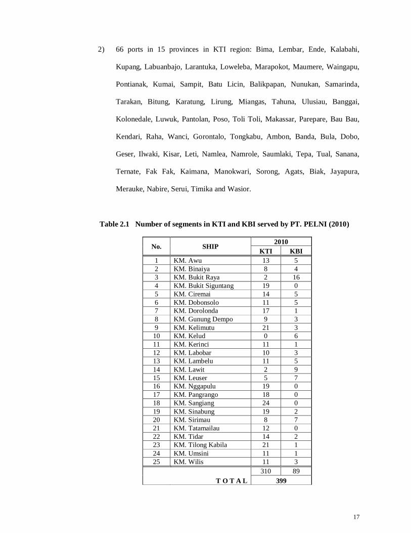
2) 66 ports in 15 provinces in KTI region: Bima, Lembar, Ende, Kalabahi,

Kupang, Labuanbajo, Larantuka, Loweleba, Marapokot, Maumere, Waingapu,

Pontianak, Kumai, Sampit, Batu Licin, Balikpapan, Nunukan, Samarinda,

Tarakan, Bitung, Karatung, Lirung, Miangas, Tahuna, Ulusiau, Banggai,

Kolonedale, Luwuk, Pantolan, Poso, Toli Toli, Makassar, Parepare, Bau Bau,

Kendari, Raha, Wanci, Gorontalo, Tongkabu, Ambon, Banda, Bula, Dobo,

Geser, Ilwaki, Kisar, Leti, Namlea, Namrole, Saumlaki, Tepa, Tual, Sanana,

Ternate, Fak Fak, Kaimana, Manokwari, Sorong, Agats, Biak, Jayapura,

Merauke, Nabire, Serui, Timika and Wasior.

Table 2.1 Number of segments in KTI and KBI served by PT. PELNI (2010)

No. SHIP 2010

KTI KBI 1 KM. Awu 13 5 2 KM. Binaiya 8 4 3 KM. Bukit Raya 2 16 4 KM. Bukit Siguntang 19 0 5 KM. Ciremai 14 5 6 KM. Dobonsolo 11 5 7 KM. Dorolonda 17 1 8 KM. Gunung Dempo 9 3 9 KM. Kelimutu 21 3

10 KM. Kelud 0 6 11 KM. Kerinci 11 1 12 KM. Labobar 10 3 13 KM. Lambelu 11 5 14 KM. Lawit 2 9 15 KM. Leuser 5 7 16 KM. Nggapulu 19 0 17 KM. Pangrango 18 0 18 KM. Sangiang 24 0 19 KM. Sinabung 19 2 20 KM. Sirimau 8 7 21 KM. Tatamailau 12 0 22 KM. Tidar 14 2 23 KM. Tilong Kabila 21 1 24 KM. Umsini 11 1 25 KM. Wilis 11 3

310 89 T O T A L 399

18

The sea depth of each port may differ from the other as shown in Appendix A.3. There

are 12 fuel ports in Indonesia namely Ambon, Balikpapan, Belawan, Benoa, Bitung,

Kupang, Makassar, Pontianak, Semarang, Surabaya, Tanjung Priok and Ternate (PELNI,

2010).

2.2 Ship

Ships operate between ports and are used for loading and unloading of cargo and

passengers. They also need to load fuel, fresh water, and supplies, as well as to discharge

waste. Ports impose physical limitations on the dimensions of the ships (ship draft,

length and width), and charge fees for their services.

Ships come in a variety of types for different uses and it can be categorised based on

(Japan International Corporation Agency, 2004):

1) Cargo ship

Cargo ships can be classified as followed:

Container ships are cargo ships that transport their entire load in truck-size

containers, in a technique called containerisation. They form a common means of

commercial inter-modal freight transport.

Bulk carriers are cargo ships used to transport bulk cargo items such as ore or

food staples (rice, grain, etc.). A bulk carrier could be either dry or wet.

Tankers are cargo ships for the transportation of fluids, such as petroleum

products, chemicals, and vegetable oils.

2) Passenger ship

Most passenger ships operate on regular, frequent and return services. Passenger

ships are part of the public transport systems of many waterside cities and islands.

19

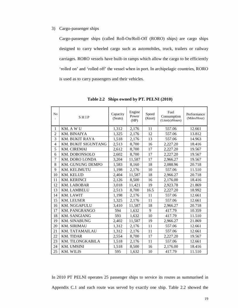
3) Cargo-passenger ships

Cargo-passenger ships (called Roll-On/Roll-Off (RORO) ships) are cargo ships

designed to carry wheeled cargo such as automobiles, truck, trailers or railway

carriages. RORO vessels have built-in ramps which allow the cargo to be efficiently

‘rolled on’ and ‘rolled off’ the vessel when in port. In archipelagic countries, RORO

is used as to carry passengers and their vehicles.

Table 2.2 Ships owned by PT. PELNI (2010)

No.

Capacity (Seats)

Engine Power (HP)

Speed (Knot)

Fuel Consumption (Liter(s)/Hours)

Performance (Miles/Hour) S H I P

1 KM. A W U 1,312 2,176 11 557.06 12.661 2 KM. BINAIYA 1,325 2,176 12 557.06 13.812 3 KM. BUKIT RAYA 1,518 2,176 13 557.06 14.963 4 KM. BUKIT SIGUNTANG 2,513 8,700 16 2,227.20 18.416 5 KM. CIREMAI 2,612 8,700 17 2,227.20 19.567 6 KM. DOBONSOLO 2,602 8,700 17 2,227.20 19.567 7 KM. DORO LONDA 3,204 11,587 17 2,966.27 19.567 8 KM. GUNUNG DEMPO 1,583 8,160 18 2,088.96 20.718 9 KM. KELIMUTU 1,198 2,176 10 557.06 11.510

10 KM. KELUD 2,404 11,587 18 2,966.27 20.718 11 KM. KERINCI 2,126 8,500 16 2,176.00 18.416 12 KM. LABOBAR 3,018 11,421 19 2,923.78 21.869 13 KM. LAMBELU 2,513 8,700 16.5 2,227.20 18.992 14 KM. LAWIT 1,198 2,176 11 557.06 12.661 15 KM. LEUSER 1,325 2,176 11 557.06 12.661 16 KM. NGGAPULU 3,410 11,587 18 2,966.27 20.718 17 KM. PANGRANGO 594 1,632 9 417.79 10.359 18 KM. SANGIANG 593 1,632 10 417.79 11.510 19 KM. SINABUNG 2,402 11,587 19 2,966.27 21.869 20 KM. SIRIMAU 1,312 2,176 11 557.06 12.661 21 KM. TATAMAILAU 1,312 2,176 11 557.06 12.661 22 KM. TIDAR 2,554 8,700 17 2,227.20 19.567 23 KM. TILONGKABILA 1,518 2,176 11 557.06 12.661 24 KM. UMSINI 1,518 8,500 16 2,176.00 18.416 25 KM. WILIS 595 1,632 10 417.79 11.510

In 2010 PT PELNI operates 25 passenger ships to service its routes as summarised in

Appendix C.1 and each route was served by exactly one ship. Table 2.2 showed the

20

capacity, engine power, speed, fuel consumption per hour, and performance of ships

used.

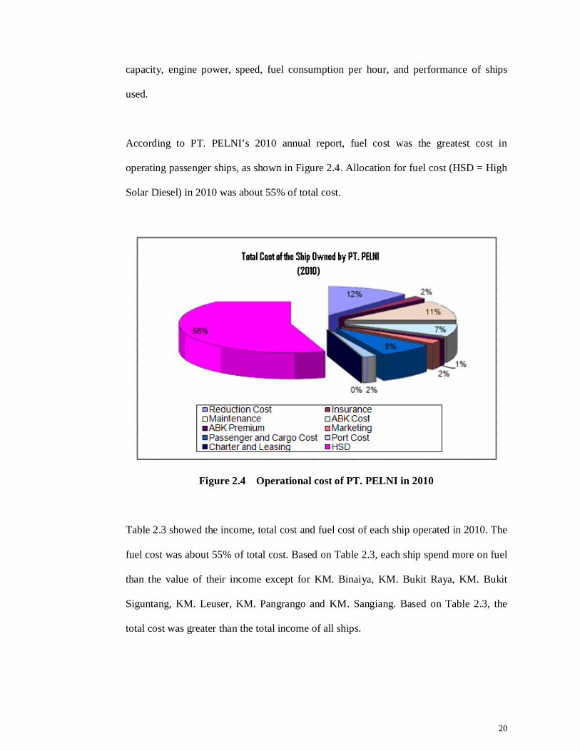
According to PT. PELNI’s 2010 annual report, fuel cost was the greatest cost in

operating passenger ships, as shown in Figure 2.4. Allocation for fuel cost (HSD = High

Solar Diesel) in 2010 was about 55% of total cost.

Figure 2.4 Operational cost of PT. PELNI in 2010

Table 2.3 showed the income, total cost and fuel cost of each ship operated in 2010. The

fuel cost was about 55% of total cost. Based on Table 2.3, each ship spend more on fuel

than the value of their income except for KM. Binaiya, KM. Bukit Raya, KM. Bukit

Siguntang, KM. Leuser, KM. Pangrango and KM. Sangiang. Based on Table 2.3, the

total cost was greater than the total income of all ships.

21

Table 2.3 Income and cost of the ships owned by PT. PELNI in 2010

22

2.3 Passenger

The population of the KTI region is approximately 44,737,300 people with a land area of

about 1,294,919.70 km2. Meanwhile, the population of the KBI region is approximately

189,428,600 people, with a land area of about 616,011.62 km2 (Statistik, 2010). The

average population density in KTI is 35 people/km2 and in KBI it is about 308

people/km2.

Table 2.4 shows the number of embarkations and disembarkations of passengers in each

province in 2010. The total number of passengers was 8,881,436; of which 7,090,147

(80 %) were from the KTI region and 1,791,289 (20 %) were from the KBI region. This

shows that passengers in the KTI region dominated the services of PT. PELNI.

23

Table 2.4 Passenger distribution based on province

24

We conducted a survey on PT. PELNI’s passenger ships between June and September

2011. Samples were recorded in June 2011, July 2012, and September 2012. These

periods were chosen because June 2011 represented average days, July 2011 represented

school holidays, and September 2011 represented the peak time (Ied). The total number

of respondents was 500, of which 17 could not be used (invalid).

The distribution of samples was comprised of 30 % from KM. Lambelu, 30 % from KM.

Kelud, and 40% from KM. Bukit Raya. KM. Lambelu sailed within the KTI region,

KM. Kelud sailed within the KBI region, and KM. Bukit Raya sailed within both of

these regions. The results of the survey, which show the characteristics of PT. PELNI’s

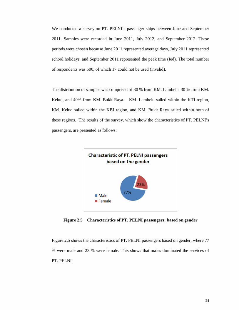
passengers, are presented as follows:

Figure 2.5 Characteristics of PT. PELNI passengers; based on gender

Figure 2.5 shows the characteristics of PT. PELNI passengers based on gender, where 77

% were male and 23 % were female. This shows that males dominated the services of

PT. PELNI.

25

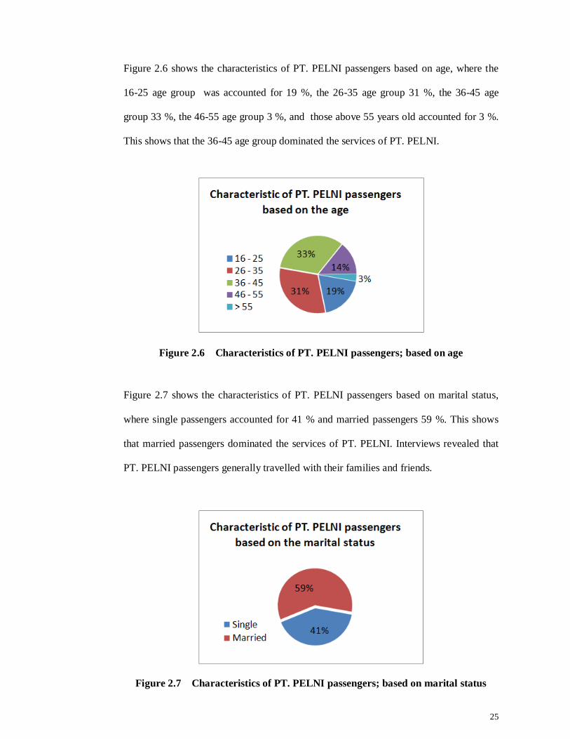
Figure 2.6 shows the characteristics of PT. PELNI passengers based on age, where the

16-25 age group was accounted for 19 %, the 26-35 age group 31 %, the 36-45 age

group 33 %, the 46-55 age group 3 %, and those above 55 years old accounted for 3 %.

This shows that the 36-45 age group dominated the services of PT. PELNI.

Figure 2.6 Characteristics of PT. PELNI passengers; based on age

Figure 2.7 shows the characteristics of PT. PELNI passengers based on marital status,

where single passengers accounted for 41 % and married passengers 59 %. This shows

that married passengers dominated the services of PT. PELNI. Interviews revealed that

PT. PELNI passengers generally travelled with their families and friends.

Figure 2.7 Characteristics of PT. PELNI passengers; based on marital status

26

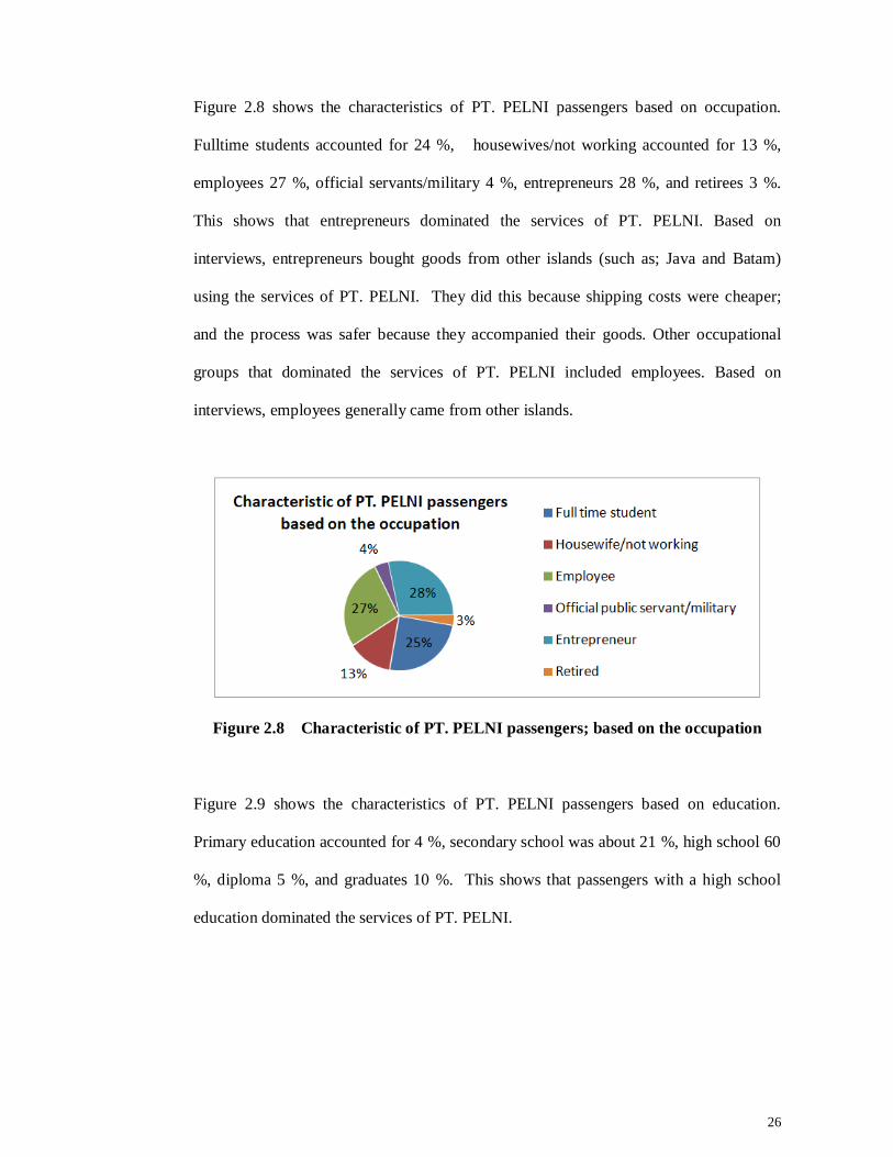
Figure 2.8 shows the characteristics of PT. PELNI passengers based on occupation.

Fulltime students accounted for 24 %, housewives/not working accounted for 13 %,

employees 27 %, official servants/military 4 %, entrepreneurs 28 %, and retirees 3 %.

This shows that entrepreneurs dominated the services of PT. PELNI. Based on

interviews, entrepreneurs bought goods from other islands (such as; Java and Batam)

using the services of PT. PELNI. They did this because shipping costs were cheaper;

and the process was safer because they accompanied their goods. Other occupational

groups that dominated the services of PT. PELNI included employees. Based on

interviews, employees generally came from other islands.

Figure 2.8 Characteristic of PT. PELNI passengers; based on the occupation

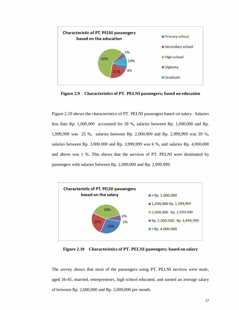
Figure 2.9 shows the characteristics of PT. PELNI passengers based on education.

Primary education accounted for 4 %, secondary school was about 21 %, high school 60

%, diploma 5 %, and graduates 10 %. This shows that passengers with a high school

education dominated the services of PT. PELNI.

27

Figure 2.9 Characteristics of PT. PELNI passengers; based on education

Figure 2.10 shows the characteristics of PT. PELNI passengers based on salary. Salaries

less than Rp. 1,000,000 accounted for 39 %, salaries between Rp. 1,000,000 and Rp.

1,999,999 was 25 %, salaries between Rp. 2,000,000 and Rp. 2,999,999 was 39 %,

salaries between Rp. 3.000.000 and Rp. 3,999,999 was 6 %, and salaries Rp. 4,000,000

and above was 1 %. This shows that the services of PT. PELNI were dominated by

passengers with salaries between Rp. 2,000,000 and Rp. 2,999,999.

Figure 2.10 Characteristics of PT. PELNI passengers; based on salary

The survey shows that most of the passengers using PT. PELNI services were male,

aged 36-45, married, entrepreneurs, high school educated, and earned an average salary

of between Rp. 2,000,000 and Rp. 3,000,000 per month.

28

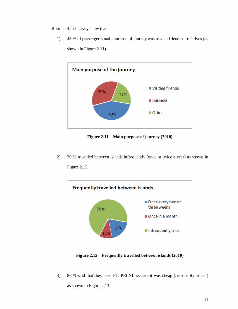
Results of the survey show that:

1) 43 % of passenger’s main purpose of journey was to visit friends or relatives (as

shown in Figure 2.11).

Figure 2.11 Main purpose of journey (2010)

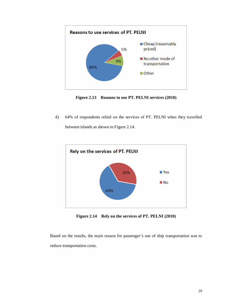
2) 70 % travelled between islands infrequently (once or twice a year) as shown in

Figure 2.12.

Figure 2.12 Frequently travelled between islands (2010)

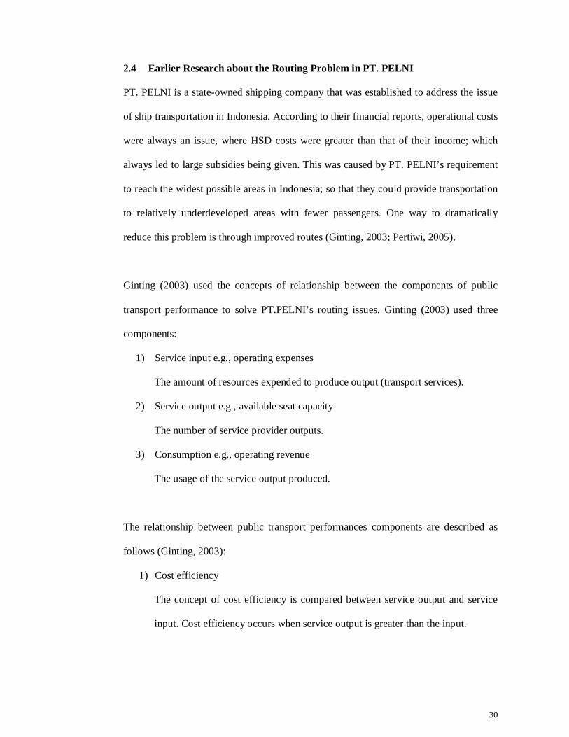
3) 86 % said that they used PT. PELNI because it was cheap (reasonably priced)

as shown in Figure 2.13.

29

Figure 2.13 Reasons to use PT. PELNI services (2010)

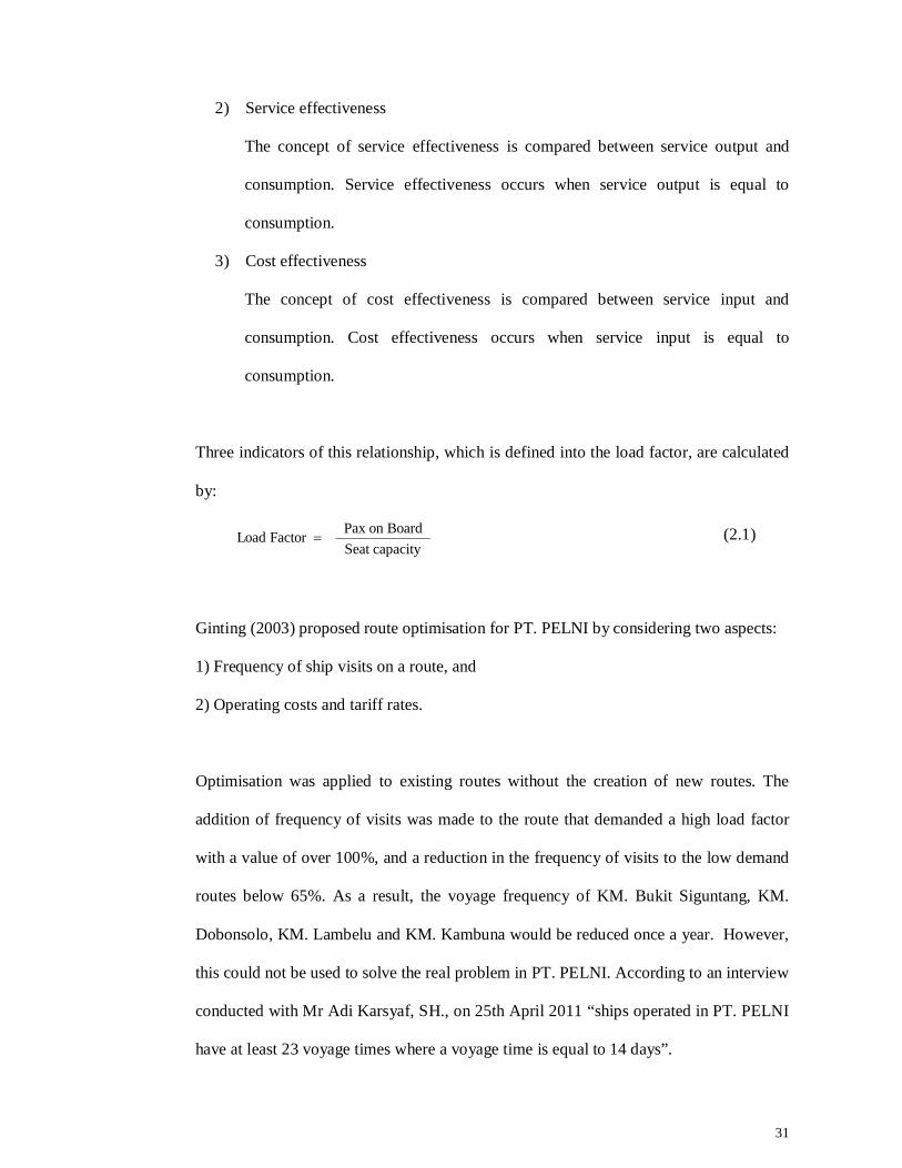
4) 64% of respondents relied on the services of PT. PELNI when they travelled

between islands as shown in Figure 2.14.

Figure 2.14 Rely on the services of PT. PELNI (2010)

Based on the results, the main reason for passenger’s use of ship transportation was to

reduce transportation costs.

30

2.4 Earlier Research about the Routing Problem in PT. PELNI

PT. PELNI is a state-owned shipping company that was established to address the issue

of ship transportation in Indonesia. According to their financial reports, operational costs

were always an issue, where HSD costs were greater than that of their income; which

always led to large subsidies being given. This was caused by PT. PELNI’s requirement

to reach the widest possible areas in Indonesia; so that they could provide transportation

to relatively underdeveloped areas with fewer passengers. One way to dramatically

reduce this problem is through improved routes (Ginting, 2003; Pertiwi, 2005).

Ginting (2003) used the concepts of relationship between the components of public

transport performance to solve PT.PELNI’s routing issues. Ginting (2003) used three

components:

1) Service input e.g., operating expenses

The amount of resources expended to produce output (transport services).

2) Service output e.g., available seat capacity

The number of service provider outputs.

3) Consumption e.g., operating revenue

The usage of the service output produced.

The relationship between public transport performances components are described as

follows (Ginting, 2003):

1) Cost efficiency

The concept of cost efficiency is compared between service output and service

input. Cost efficiency occurs when service output is greater than the input.

31

2) Service effectiveness

The concept of service effectiveness is compared between service output and

consumption. Service effectiveness occurs when service output is equal to

consumption.

3) Cost effectiveness

The concept of cost effectiveness is compared between service input and

consumption. Cost effectiveness occurs when service input is equal to

consumption.

Three indicators of this relationship, which is defined into the load factor, are calculated

by:

capacitySeat

Boardon Pax Factor Load (2.1)

Ginting (2003) proposed route optimisation for PT. PELNI by considering two aspects:

1) Frequency of ship visits on a route, and

2) Operating costs and tariff rates.

Optimisation was applied to existing routes without the creation of new routes. The

addition of frequency of visits was made to the route that demanded a high load factor

with a value of over 100%, and a reduction in the frequency of visits to the low demand

routes below 65%. As a result, the voyage frequency of KM. Bukit Siguntang, KM.

Dobonsolo, KM. Lambelu and KM. Kambuna would be reduced once a year. However,

this could not be used to solve the real problem in PT. PELNI. According to an interview

conducted with Mr Adi Karsyaf, SH., on 25th April 2011 “ships operated in PT. PELNI

have at least 23 voyage times where a voyage time is equal to 14 days”.

32

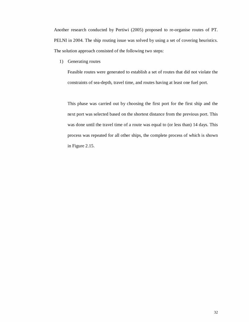
Another research conducted by Pertiwi (2005) proposed to re-organise routes of PT.

PELNI in 2004. The ship routing issue was solved by using a set of covering heuristics.

The solution approach consisted of the following two steps:

1) Generating routes

Feasible routes were generated to establish a set of routes that did not violate the

constraints of sea-depth, travel time, and routes having at least one fuel port.

This phase was carried out by choosing the first port for the first ship and the

next port was selected based on the shortest distance from the previous port. This

was done until the travel time of a route was equal to (or less than) 14 days. This

process was repeated for all other ships, the complete process of which is shown

in Figure 2.15.

33

Figure 2.15 Generating routes in Pertiwi (2005)

34

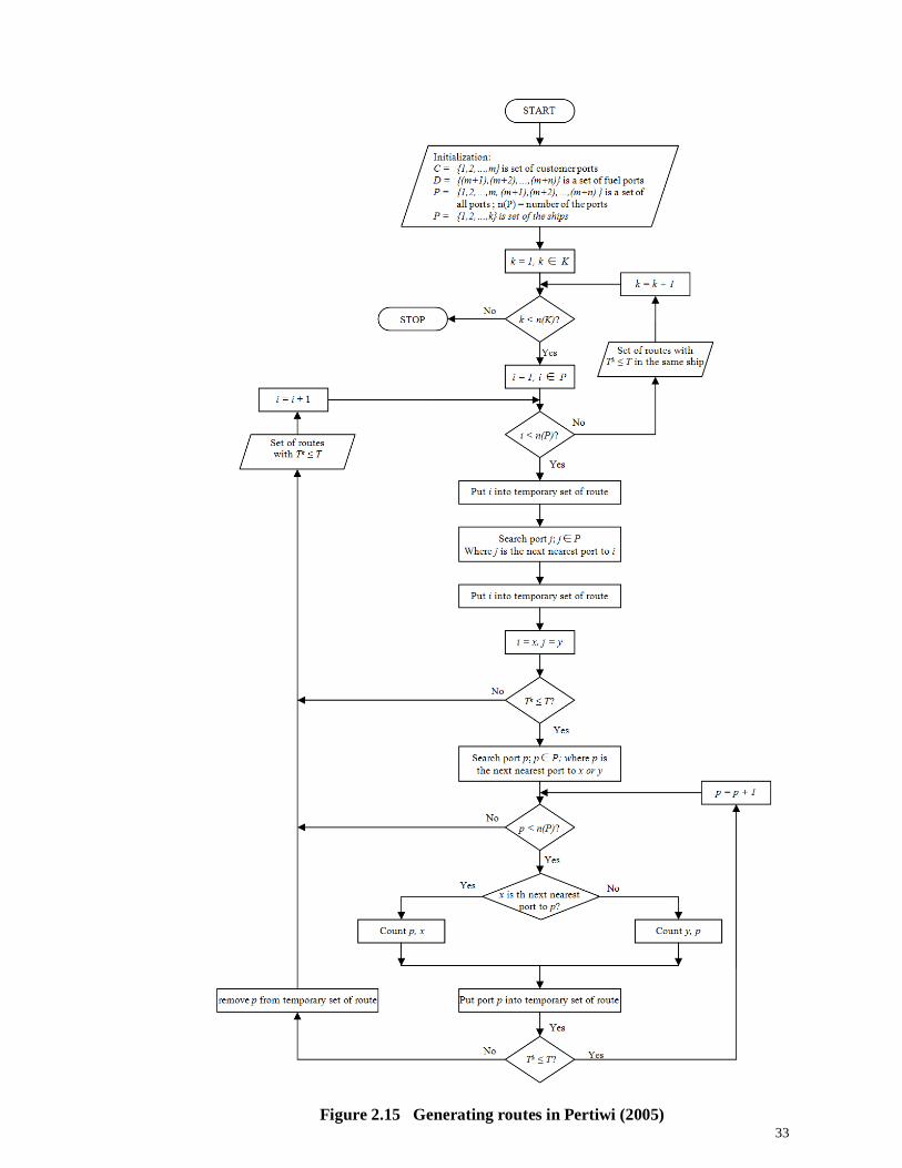
2) Choosing the best routes

This phase aimed to choose a set of routes that satisfied constraints with

minimum cost. A penalty would be imposed for routes that violated one or more

constraints.

This phase was carried out by choosing the best combination of routes that

served all of the ports and used all of the ships. The process of choosing the best

routes is shown in Figure 2.16.

Figure 2.16 Choosing the best routes in Pertiwi (2005)

35

According to an interview conducted with Mr. Adi Karsyaf SH on 25th April 2011, he

said that there are some disadvantages to the algorithm proposed by Pertiwi (2005),

namely:

1) The travel distance is ignored.

PT. PELNI operates different types of ships; therefore, the fuel tank capacity of

each ship is different. Since the fuel tank capacity of each ship is different the

maximum travel distance of each ship would also be different.

2) The load factor is ignored.

The ideal load factor in PT. PELNI is 65 %.

3) The number of ports of call is ignored.

Since the number of ports of call is ignored, the route made is not supportive of

the vision of PT. PELNI (could not be applied into a real situation in PT.

PELNI).

In the research by Pertiwi (2005), the goal was to minimise the total voyage cost where

the load factor and number of ports of call would be ignored. The solution produced

offered to lower the total voyage cost by 9.72 %; compared to the existing 2004 route.

2.5 Summary

In this chapter, we discussed our case study i.e., PT. PELNI. The two most important

parts of the PT. PELNI study are accessibility and profitability. Accessibility usually

reduces profit, while an increase in profit tends to reduce accessibility. To increase

profit, a route needs to have minimum fuel consumption, which affects the number of

ports of call. PT. PELNI’s ships use a High Solar Diesel (HSD) fuel and PT. PELNI

spent 55 % of their total costs on for fuel in 2010.

36

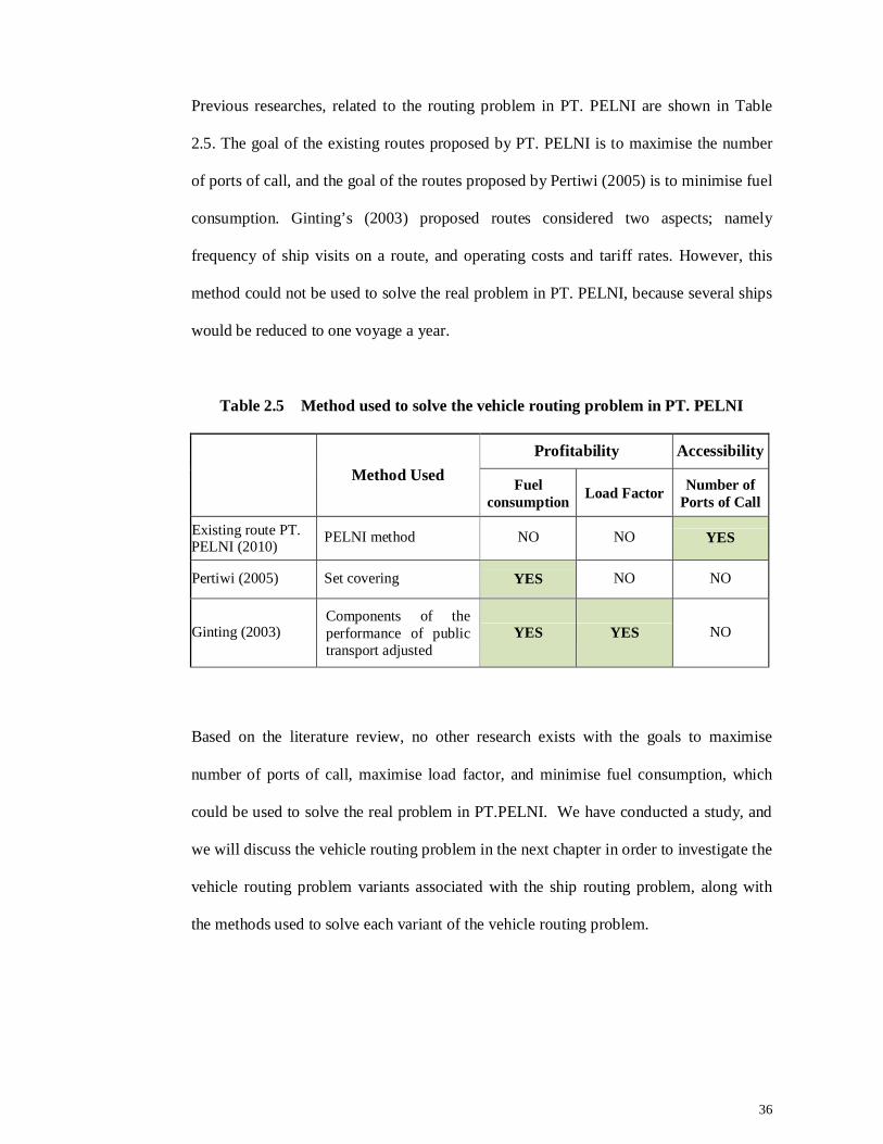
Previous researches, related to the routing problem in PT. PELNI are shown in Table

2.5. The goal of the existing routes proposed by PT. PELNI is to maximise the number

of ports of call, and the goal of the routes proposed by Pertiwi (2005) is to minimise fuel

consumption. Ginting’s (2003) proposed routes considered two aspects; namely

frequency of ship visits on a route, and operating costs and tariff rates. However, this

method could not be used to solve the real problem in PT. PELNI, because several ships

would be reduced to one voyage a year.

Table 2.5 Method used to solve the vehicle routing problem in PT. PELNI

Method Used Profitability Accessibility

Fuel consumption Load Factor Number of

Ports of Call

Existing route PT. PELNI (2010) PELNI method NO NO YES

Pertiwi (2005) Set covering YES NO NO

Ginting (2003) Components of the performance of public transport adjusted

YES YES NO

Based on the literature review, no other research exists with the goals to maximise

number of ports of call, maximise load factor, and minimise fuel consumption, which

could be used to solve the real problem in PT.PELNI. We have conducted a study, and

we will discuss the vehicle routing problem in the next chapter in order to investigate the

vehicle routing problem variants associated with the ship routing problem, along with

the methods used to solve each variant of the vehicle routing problem.

37

CHAPTER 3 VEHICLE ROUTING PROBLEM

A vehicle routing problem is a general combinatorial optimization problem that has

become a key component of transportation management. Dantzig & Ramser (1959) first

introduced vehicle routing problems. General vehicle routing problems are defined on

connected graph G. Let G = (V, A) be a graph where V is a set of nodes (vertices) and A

is the set of arcs (edges). Let C = (cij) be a cost matrix associated with A. The matrix C is

symmetric when cij = cji and asymmetric otherwise.

A general vehicle routing problem consists of determining several vehicle routes with

the minimum cost for serving a set of customers, whose geographical coordinates and

demands are known in advance. A vehicle visits each customer only once. Typically,

vehicles are homogeneous and have the same capacity restrictions. The vehicle must

start and finish its tour at the depot, and the problem is to construct a route at the

minimum travel cost. The VRP lies between the travelling salesman problem (TSP) and

the bin-packing problem (BPP) (Falkenauer, 1996; Lupsa et al., 2010; Reinelt, 1994).

The travelling salesman problem aims to determine the shortest tour in which all the

specified disjointed subsets of the vertices of a graph are visited. The travelling salesman

needs to visit each city exactly once, starting and ending in his home town (Bonyadi et

al., 2008; Greco & Gerace, 2008; Wei, 2008). The goal is to find the shortest tour

through all the cities. To describe a travelling salesman problem as a vehicle routing

problem, a vehicle routing problem with one depot, one vehicle with an unlimited

capacity (or set all demands to zero), a cost function proportional to only the distance,

and an arbitrary number of customers (cities) are used (Liu, 2008; Matai et al., 2010).

38

A bin-packing problem is described as follows: given a finite set of numbers (the item

sizes) and a constant to specify the capacity of the bin, determine the minimum number

of bins needed where all the items have to be inside exactly one bin and the total

capacity of the items in each bin has to be within the capacity limits of the bin. In a bin

packing problem, objects of different volumes must be packed into a finite number of

bins to suit the vehicle capacity in a way that minimizes the number of bins used. A bin-

packing problem can be described as a vehicle routing problem by considering the

variant of the vehicle routing problem with one depot and a cost matrix of all the zeroes

(Falkenauer, 1996).

Some vehicle routing problem variants and the unique constraints are:

1. Multiple Depot Vehicle Routing Problem (MDVRP)

The multiple depot vehicle routing problem is a vehicle routing problem with

multiple depots (Cordeau et al., 1997; Dondo & Cerdá, 2007; Nagy & Salhi, 2005;

Renaud et al., 1996; Salhi & Sari, 1997).

2. Capacitated Vehicle Routing Problem (CVRP)

The capacitated vehicle routing problem is a vehicle routing problem with an

additional constraint requiring all vehicles within the fleet to have a uniform

carrying capacity for a single commodity. The commodity demands along any route

assigned to a vehicle must not exceed the capacity of the vehicle. There are two

types of capacitated vehicle routing problems:

i. Homogeneous fleet vehicle routing problem

In a homogeneous fleet vehicle routing problem (or uniform fleet vehicle

routing problem), each vehicle in the fleet has the same capacity. The only

difference is that a route is considered feasible if the total demand of all the

customers on a route does not exceed the capacity Of the vehicle. The total

demand of all the customers cannot be greater than the total capacity of all

39

the vehicles, and those vehicles must be big enough, i.e. the demand of a

customer is never greater than the capacity of the vehicles (Lin et al., 2009;

Nagata & Bräysy, 2009).

ii. Heterogeneous fleet vehicle routing problem

In a heterogeneous fleet vehicle routing problem (or HVRP), the fleet is

composed of different vehicle types, each with its own capacity.

Restrictions, similar to the ones defined for the homogeneous vehicle routing

problem apply, for the maximum demand per route, and the maximum total

demand is in relation to the capacity of the vehicles (Brandão, 2011; Choi &

Tcha, 2007; Li et al., 2007; Ochi et al., 1998).

3. Site Dependent Capacitated Vehicle Routing Problem (SDCVRP)

A site dependent capacitated vehicle routing problem is a variant of the

heterogeneous capacitated vehicle routing problem where not every type of vehicle

can serve every type of customer because of site-dependent restrictions (Chao et al.,

1998; Cordeau & Laporte, 2001; Nag et al., 1988).

4. Asymmetric Vehicle Routing Problem (AVRP)

An asymmetric vehicle routing problem is a vehicle routing problem with a travel

distance from port i to port j, i.e., lij is not necessary equal to lji (Choi et al., 2003).

3.1 Multi Depot Vehicle Routing Problem

The multi-depot vehicle routing problem (MDVRP) is a general vehicle routing problem

with multiple depots. A company may have several depots from which it serves

customers. If the customers are clustered around the depots, it is possible to model these

distribution problems as a set of vehicle routing problems. However, if it isn’t clear

which customers should be served from which depot, a multi-depot vehicle routing

problem can be used to find the best solution (Nagy & Salhi, 2005; Salhi & Sari, 1997).

40

In a multi depot vehicle routing problem, each depot stores and supplies various

products, and has a number of identical vehicles with the same capacity to serve

customers who demand different quantities of various products. Each vehicle starts the

tour from its resident depot, delivers products to a number of customers, and returns to

the same depot (Cordeau et al., 1997; Renaud et al, 1996). The goal of a multi-depot

vehicle routing problem, in which the total demand of commodities is served from

several depots, is to make each route satisfy the constraints while beginning and

returning to the same.

Ho et al. (2008) proposed using a hybrid genetic algorithm to solve multi-depot vehicle

routing problem. They used three steps in the initialization, i.e. grouping, routing and

scheduling. The grouping was done based on the distance between the customers and the

depots, the routing was based on Clarke and Wright’s saving method, while the

scheduling was by the nearest neighbour heuristic. The objective was to minimise the

total delivery time spent in the distribution by assigning the customers to the nearest

depot. A computational study showed that the best results were achieved for the initial

population by using the ‘Clarke and Wright saving’ method (Clarke & Wright, 1964).

The nearest neighbours were randomly compared to the initial population.

3.2 Heterogeneous Fleet Vehicle Routing Problem

The capacitated vehicle routing problem (CVRP) is the most common and basic variant

of the vehicle routing problem. The capacitated vehicle routing problem is a generic

name given to a whole class of problems in which each vehicle has the same loading

capacity, starts from only one depot, and then routes through to a number of customers

(Lin et al., 2009).

41

A set of routes for a fleet of vehicles based together must be determined for a number of

geographically dispersed customers, and the vehicles must be loaded to the maximum

capacity. All customers have a known demand for a single commodity, each customer

can only be visited by one vehicle, and each vehicle has to return to the depot. The

service time unit can be transformed into a distance unit. The loading and travelling

distance of each vehicle cannot exceed the loading capacity and the maximum travelling

distance respectively of each vehicle. All the vehicles in the capacitated vehicle routing

problem are homogeneous and have the same capacity, while the size of the fleet is

unlimited (Nagata & Bräysy, 2009).

Many variants of the capacitated vehicle routing problem relax one or both of these

conditions. One variant of the capacitated vehicle routing problem is the heterogeneous

fleet vehicle routing problem (HVRP). In a heterogeneous fleet vehicle routing problem,

the fleet is composed of a fixed number of vehicles with differences in their equipment,

capacity, or cost, and in which the number of available vehicles is fixed as a priori

(Baldacci et al., 2008; Gendreau et al., 1999; Pessoa et al., 2009; Taillard, 1999). The

decision is how to best utilize the existing fleet to serve customer demands (Choi &

Tcha, 2007; Li et al., 2007; Prins, 2009).

Vehicle routing problems are complicated in real-life contexts when the vehicle fleets

are heterogeneous. Using a heterogeneous fleet of vehicles has multiple advantages. In

some cases, it is possible to service customers requiring small vehicles because of

accessibility restrictions. Notable examples are size and weight constraints which may

even vary over time, as exemplified by the physical dimension constraints of a ship,

including the draft restrictions of the ship that vary with the tide, the available berth

space in ports and the sea depth of ports (Ochi et al., 1998; Penna et al., 2011; Yaman,

2006; Tarantilis et al., 2004).

42

In a heterogeneous fleet, vehicles of different carrying capacities provide the flexibility

to allocate capacity according to the customers’ varying demands in a cost effective way

by deploying appropriate vehicle types to areas with analogous concentrations of

customers (Prins, 2002; Subramanian et al., 2012; Tarantilis et al., 2003).

Jeon et al., (2007) used a hybrid Genetic Algorithm to solve the heterogeneous fleet

vehicle routing problem (HVRP) and the multi-depot vehicle routing problem

(MDVRP), where the initial population method simultaneously used both an initial

solution by using a heuristic and a random generation method. The random generation

method provided solutions created from random numbers and a global search. The initial

population underwent the following techniques: a minimization process for an infeasible

solution, a gene exchange process, a route exchange process, and a flexible mutation

rate. The objective was to minimize distance and the results proved that the hybrid

genetic algorithm performed better than the general Genetic Algorithm.

3.3 Site Dependent Capacitated Vehicle Routing Problem

A site-dependent capacitated vehicle routing problem is a variant of the heterogeneous

capacitated vehicle routing problem where not every vehicle type is suitable for serving

every customer because of site-dependent restrictions (Archetti et al., (2010); Cordeau &

Laporte, 2001).

In a site-dependent capacitated vehicle routing problem, the fleet has many types of

vehicles and there are vehicle site compatibilities between the customer sites and vehicle

types. The problem consists of assigning compatible vehicle types to each customer and

designing vehicle routes for the vehicles of each type, as in a vehicle routing problem

(Chao et al., 1998; Nag et al., 1988). Chao et al. (1999) proposed an algorithm for

43

solving the dependent capacitated vehicle routing problem. The algorithm consists of

two steps: obtain a feasible solution, and improve the feasible solution via a sequence of

uphill and downhill moves.

3.4 Asymmetric Vehicle Routing Problem

An asymmetric vehicle routing problem (AVRP) is a variant of the heterogeneous

capacitated vehicle routing problem (HCVRP), where travel distance from port i to port

j, i.e., lij, does not necessary equal lji (Choi et al., 2003). An asymmetric vehicle routing

problem is related to the asymmetric travelling salesman problem (ATSP). An

asymmetric travelling salesman problem is a generalized travelling salesman problem in

which the distance between a pair of cities is not the same from the opposite direction.

3.5 Solution to the VRP

The vehicle routing problem (VRP) occurs between the travelling salesman problem

(TSP) and the bin-packing problem (BPP). The TSP and BPP are types of NP-hard

combinatorial optimization problems. Thus, the existence of a known algorithm that can

solve all cases to optimality in a reasonable execution time is not guaranteed.

Methods have been proposed for addressing the VRP. These methods are distinguished

by using heuristics and metaheuristics. Some of the widely used solutions for various

VRP combinations are illustrated in Figure 3.1.

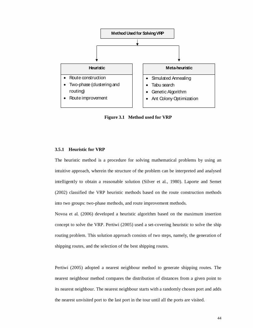
44

Figure 3.1 Method used for VRP

3.5.1 Heuristic for VRP

The heuristic method is a procedure for solving mathematical problems by using an

intuitive approach, wherein the structure of the problem can be interpreted and analysed

intelligently to obtain a reasonable solution (Silver et al., 1980). Laporte and Semet

(2002) classified the VRP heuristic methods based on the route construction methods

into two groups: two-phase methods, and route improvement methods.

Novoa et al. (2006) developed a heuristic algorithm based on the maximum insertion

concept to solve the VRP. Pertiwi (2005) used a set-covering heuristic to solve the ship

routing problem. This solution approach consists of two steps, namely, the generation of

shipping routes, and the selection of the best shipping routes.

Pertiwi (2005) adopted a nearest neighbour method to generate shipping routes. The

nearest neighbour method compares the distribution of distances from a given point to

its nearest neighbour. The nearest neighbour starts with a randomly chosen port and adds

the nearest unvisited port to the last port in the tour until all the ports are visited.

Simulated Annealing Tabu search Genetic Algorithm Ant Colony Optimization

Meta-heuristic Route construction Two-phase (clustering and

routing) Route improvement

Heuristic

Method Used for Solving VRP

45

3.5.1.1 Route Construction

Route construction methods are among the first heuristic methods for the VRP and are

still implemented for several routing applications. These algorithms typically start from

an empty solution and construct routes iteratively by inserting one or more customers

until all the customers are served. Route construction methods have three primary

components:

1. Initialization criterion

2. Selection criterion that specifies which customers are chosen for insertion at the

current iteration

3. Insertion criterion to determine the location of chosen customers in the current

routes

A heuristic approach in the route construction method is the saving algorithm. This

algorithm was proposed by Clarke & Wright (1964). The saving algorithm is based on

the concept of saving an estimate of the cost reduction obtained by sequentially serving

two customers in the same route rather than in two separate routes. If i is the last

customer of a route and j is the first customer of another route, the associated saving is

defined as sij = ci0 + c0j − cij.

The steps in the saving algorithm process are as follows:

Step 1: n dedicated routes (round trips that service only one store) are determined;

one route corresponds to one n store.

Step 2: Savings in distance, sij, are computed by combining every possible pair of

stores into one: sij = ci0 + c0j − cij

Step 3: Savings are ordered in a decreasing fashion. Given that negative S values are

undesirable, negative values are omitted from the list.

46

Step 4: A route is built by adding pairs that do not violate any of the set constraints

in order to allow the pairs to appear in the list until the route is full or until

the list has been exhausted. The resulting suppliers form a cluster.

Step 5: Step 4 is repeated until all the stores are routed or until the list has been

exhausted.

3.5.1.2 Two Phase (Clustering and Routing) Method

Two-phase methods are based on the decomposition of the VRP solution process into

two separate sub problems:

1. Clustering

The partition of customers is defined as subsets that correspond to a route.

2. Routing

The sequence of customers is determined on each route.

In a cluster first - route second method, customers are first grouped into clusters, and the

routes are determined by appropriately sequencing the customers within each cluster. In

a route first - cluster second method, a giant tour of all the customers is constructed in

the first phase and then subdivided into feasible routes.

A. Cluster First - Route Second Method

Different techniques have been proposed for the clustering phase, where the

cluster first - route second method is employed in the routing phase. The sweep

algorithm is often considered a cluster first - route second approach. This

algorithm was developed by Gillett & Miller (1974), Wren (1971), and Wren &

Holliday (1972).

47

The algorithm begins with an arbitrary customer and then sequentially assigns the

remaining customers to the current vehicle. The assignment is accomplished by

considering customers in the order of increasing polar angles with respect to the

depot and the initial customer. If the assignment of the current customer to the

current vehicle is not feasible, a new route is initialized for the current customer.

Once all the customers are assigned to the vehicles, each route is defined

separately by solving a vehicle routing problem.

Another algorithm under the cluster first - route second approach is the truncated

branch-and-bound method developed by Christofides et al. (1979). In this

algorithm, a set of routes is determined through an adaptation of an exact branch-

and-bound algorithm that employs a branching-on-routes strategy. The decision

tree contains as many levels as the number of available vehicles. At each level of

the decision tree, a given node corresponds to a partial solution that is composed of

complete routes. The descendant nodes correspond to all possible routes including

a subset of the un-routed customers. The running time of the algorithm is

controlled by limiting the number of routes generated at each level to one.

B. Route First - Cluster Second Method

The route first - cluster second method is an alternative method for solving the

vehicle routing problem. It starts from the route construction phase. In the route

construction, the path representation encodes a unique, big journey that serves all

the customers. The second step is clustering. The clustering procedure starts from

an initial solution obtained based on the route construction phase, and it is

clustered into feasible routes. The clustering procedure attempts to find a better

neighbouring solution in terms of the number of vehicles, while maintaining

solution feasibility (Beasley, 1983). Beasley (1983), Haimovich & Kan (1985),

48

and Bertsimas & Simchi-Levi (1996) provided several examples of algorithms

classified under the route first -cluster second method.

3.5.1.3 Route Improvement

The problem in route improvement is the improvement of initial solutions generated by

other heuristics. This problem can be solved by a Local Search algorithm. A Local

Search algorithm starts from a given solution; hence, a Local Search method applies

simple modifications, such as arc exchanges or customer movements, to obtain the

neighbouring solutions efficiently. If an improved solution is identified, the new solution

is used as the current solution and the process iterates; otherwise a local minimum is

identified (Lin, 1965).

3.5.2 Metaheuristic for VRP

The word metaheuristic is derived from two Greek words: “heuristic” which means “to

find” and “meta” which means “in an upper level.” A metaheuristic is a high-level

problem-independent algorithmic framework that provides a set of guidelines or

strategies to develop heuristic optimization algorithms. Nowadays, metaheuristics are

widely used to solve important practical combinatorial optimization problems. Several

metaheuristics have been applied to the vehicle routing problem, e.g. Simulated

Annealing (Kuo, 2010), Tabu Search (Lin et al., 2009), Genetic Algorithms (Liu et. al.,

2009), and Ant Colony Optimization (Mazzeo & Loiseau 2004).

A. Simulated Annealing

Simulated Annealing is derived from the annealing process, in which a solid is

heated until it melts. Subsequently, the temperature is slowly decreased (according

49

to the annealing schedule) until the solid reaches the lowest energy or ground state.

If the initial temperature decreases rapidly, the solid in the ground state will

contain defects or imperfections. The simple implementation of the simulated

annealing algorithm, which usually provides a local search with better results,

facilitates its adoption into local search methods (e.g. the best improvement local

search). However, although the algorithm has been proven to converge to the

optimum, it converges in infinite time. Thus, in addition to the slow cooling

requirements of the solid, this algorithm is not as fast as its counterparts

(Kirkpatrick et al., 1983).

Kuo (2010) used the Simulated Annealing to solve the vehicle routing problem.

The Simulated Annealing model requires the temperature to be cooled at each

iteration. To decide on the initial temperature and the final temperature, Kuo

(2010) applied the Simulated Annealing as follows:

Choose temporary Simulated Annealing parameters.

Use the temporary Simulated Annealing parameters to solve the proposed

problem with several different initial solutions.

Let Zmax be the maximum value when using different initial solutions to

maximize the proposed problem.

Let Zmin be the minimum value when using different initial solutions to

minimize the proposed problem.

Let e(-(Zmax- Zmin)/U) = 0.5 and e(-(Zmax- Zmin)x0.0001/UA) = 0.05, then find U and UA

where; U is the initial temperature and UA is the final temperature.

B. Tabu Search

Glover proposed the Tabu Search in 1986 (Brandao, 2011; Zachariadis et al.,

2009). The word ”taboo” is derived from Tongan, which is a Polynesian language,

50

used by natives of the island of Tonga to refer to holy objects that cannot be

touched. The basic principle of the Tabu Search is to pursue the best improvement

of the Local Search whenever the latter encounters a local minimum by allowing

non-improving moves. The rule employed in defining neighbourhoods is important

to most local search heuristics (Gendreau et al., 1994; Gendreau et al., 2006;

Glover, 1990; Osman, 1993).

Lin et al., (2009) used the Simulated Annealing method and combined it with the

Tabu Search to solve the vehicle routing problem. Let,

X be generated using neighbourhood algorithm;

Xbest be the current best solution;

Y be the next solution;

Fx be the objective function value of X;

Fcur be the current objective function; and

T be the current temperature.

First, the current temperature T is set to T0 for the proposed algorithm. Next, an

initial solution, X, is generated by a neighbourhood algorithm. The current best

solution, Xbest, is set to be equal to X, and the current objective function value, Fcur,

is set to be equal to the objective function value Fx of X. The obtained best

objective function value, Xbest, is set to be equal to Fcur. For each iteration, the next

solution Y is generated from X either by swap or by insertion where the new

solution Y cannot belong to the Tabu move unless a new solution Y is the best

solution found so far. T is decreased after running Iiter iterations from the previous

decrease, according to the formula T ←αT, where 0 < α < 1. The tenure of tabu

move is reassigned by choosing an integral value when T is decreased once. The

Tabu Search is terminated when a number of added moves are performed without

any improvement over the best objective function value.

51

C. Genetic Algorithm

The Genetic Algorithm is derived from Darwin’s Theory of Natural Selection and

Mandel’s work on genetics and inheritance. The Genetic Algorithm uses a

stochastic search technique based on the mechanism of natural selection and

natural genetics (Goldberg, 1989). The Genetic Algorithm differs from

conventional search techniques because it begins with an initial set of random

solutions called a population. Each individual in the population is called a

chromosome, which represents a solution to the problem at hand.

Liu et. al. (2009) used the Genetic Algorithm to solve the vehicle routing problem.

To populate the initial population, some of the chromosomes are generated as

random sequences, and some by heuristics. The savings algorithm and the sweep

algorithm are adapted. The tournament selection is chosen as the selection process.

It is runs a tournament among a few individuals chosen at random from the

population and selects the one with the best fitness. Individual chromosomes are

ranked by their total cost. A chromosome with a smaller total cost has a better

fitness. In Liu et. al. (2009), a string relocation, string crosses and a string

exchange were used for the mutation, while an order crossover (OX) was used for

the crossover.

D. Ant Colony Optimization

While walking from the food source toward the nest; and vice versa, ants deposit a

substance called pheromone on the ground. This behaviour allows ants to

determine the shortest path between the nest and the food source. When ants

decide on the direction to follow, they choose the path that is characterized by a

high probability level of pheromone concentration. This behaviour is the basis for

the cooperative interactions that lead to the emergence of the shortest path

52

(Bianchi, 2006; Branke & Guntsch, 2004; Bullnheimer et al., 1999; Colorni et al.,

1991; Dorigo & Stutzle, 2004; Fuellerer et al., 2009; Li et al., 2009).

Mazzeo & Loiseau (2004) used the Ant Colony Optimization for solving the

capacitated vehicle routing problem and the details are provided as follows:

Step 1: Route building

In each iteration of the Ant Colony Optimization each ant builds a

solution for the route, moving to the next client (stated in the general

Ant Colony Optimization scheme) according to the transition rules

based on a combination of the amount of pheromone at each arc.

Step 2: Transition rules

A neighbour client is randomly chosen according to the probability

Pk (i, j), where k is the number of vehicles starting with customer i

and stopping with customer j.

Step 3: Pheromone actualization

There are two types of actualization; global actualization and local

actualization. Global actualization is done after each iteration is

completed, while local actualization is done each time an ant moves

from customer i to the next customer j to decrease the amount of

pheromone of a used edge (i,j) in order to diversify the solutions

obtained by the ants.

Step 4: Reduced neighbour list

This is needed when the problem is too big for all the potential moves

of the ant to be explored. A reduced list of best candidates is then

used.

53

Step 5: Improved heuristics

Improved heuristics are used to modify the ant solutions after each

iteration.

Step 6: Stopping rules

The Ant Colony Optimization procedure stops when there is no

improvement to the solution after several iterations or when the

number of iterations is reached.

3.6 Genetic Algorithm

In a Genetic Algorithm, the problem to be optimized must be stated in the objective

function and it is called fitness. The individual with the best fitness value is given a high

probability to reproduce in the next generation. For each generation in the evolutionary

process, the best fitness value is referred to as the optimal solution.

The methodology of a general Genetic Algorithm is illustrated in Figure 3.2. The

process follows five steps:

Step 1: Generate a population, including chromosomes

Step 2: Evaluate each chromosome

Step 3: Selection process to choose chromosome with the best fitness

Step 4: Manipulation for generating a new population of the current population

Step 5: Return to step 2 and step 3 for n number of iterations. The process ends after

the stopping criteria are met.

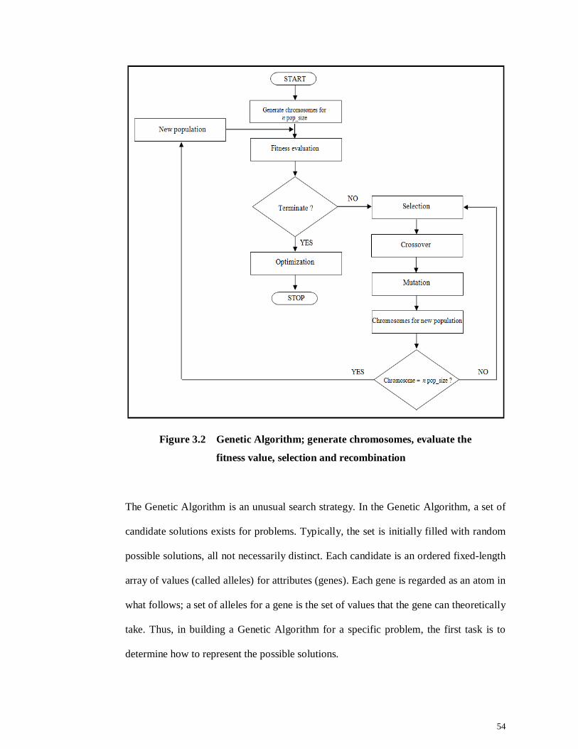
54

Figure 3.2 Genetic Algorithm; generate chromosomes, evaluate the

fitness value, selection and recombination

The Genetic Algorithm is an unusual search strategy. In the Genetic Algorithm, a set of

candidate solutions exists for problems. Typically, the set is initially filled with random

possible solutions, all not necessarily distinct. Each candidate is an ordered fixed-length

array of values (called alleles) for attributes (genes). Each gene is regarded as an atom in

what follows; a set of alleles for a gene is the set of values that the gene can theoretically

take. Thus, in building a Genetic Algorithm for a specific problem, the first task is to

determine how to represent the possible solutions.

55

Chromosomes evolve through successive iterations called generations. The

chromosomes with the highest fitness have the highest probability of being selected.

After several generations, the algorithm selects the best chromosome, which is hoped to

be the optimal solution to the problem. Two such mechanisms that link a Genetic

Algorithm to the solved problem are a method of encoding solutions to the problem on

chromosomes, and an evaluation function that returns a measurement of the worth of any

chromosomes in the context of the problem.

During each generation, the chromosomes are evaluated using some measures of fitness.

In each generation, all the chromosomes go through the processes of:

1. Evaluation

Using some predefined problem-specific measure of fitness, every member of the

current set is evaluated to determine how good a solution it is to the problem. The

measurement is called the candidate’s fitness, and the idea is that the fitter the

candidates are, the closer they are to being the sought after solution. However, the

Genetic Algorithm does not require fitness to be a perfect measure of quality; often,

poor solutions are assigned high fitness scores, despite being the less effective

solution.

2. Selection

Pairs of candidate solutions are selected to form the current generation used for

breeding. This may be done entirely randomly or stochastically based on fitness.

3. Breeding

New individuals are produced using genetic operators on the individuals chosen in

the selection step. There are two main kinds of operators:

a. Merging two chromosomes from the current generation using a crossover

operator where a new individual is produced by recombining the features of a

pair of parents’ solutions.

56

b. Modifying a chromosome using a mutation operator, where a new individual is

produced by slightly altering an existing one.

4. Recombination

The set is altered, typically by choosing to remove some or all of the individuals in

the existing generation (usually beginning with the least fit) and replacing these with

individuals produced in the breeding step. A population update is needed to keep the

population size constant. The new population produced thus becomes the current

generation.

The Genetic Algorithm has been reported to successfully solve the vehicle routing

problem. Lau et al. (2010) compared the performance of four algorithms, namely the

Branch and Bound algorithm (BB), the Simulated Annealing algorithm (SA), the Tabu

Search algorithm (TS), and the Genetic Algorithm (GA). Tests were conducted for 25

depots and 250 customers. All the results are summarized in Table 3.1.

Table 3.1 Comparison of four algorithms (Lau et al., 2010)

NO. TOTAL COST

BB SA TS GA

1 58379.31 54368.57 56229.26 51508.97

2 59264.72 52153.39 54384.11 51692.06

3 58103.46 53686.48 54921.08 50438.02

4 59759.41 53981.97 56537.65 49859.48

5 61037.95 52649.06 55446.69 50294.93

6 60648.28 51979.13 55263.52 48327.65

7 59519.53 54876.55 56785.27 51096.49

8 60229.11 53360.82 54276.68 49774.34

9 59398.03 52007.58 55894.92 50836.72

10 61645.27 51264.19 54690.81 48970.26

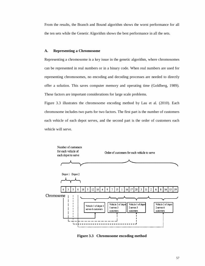
57

From the results, the Branch and Bound algorithm shows the worst performance for all

the ten sets while the Genetic Algorithm shows the best performance in all the sets.

A. Representing a Chromosome

Representing a chromosome is a key issue in the genetic algorithm, where chromosomes

can be represented in real numbers or in a binary code. When real numbers are used for

representing chromosomes, no encoding and decoding processes are needed to directly

offer a solution. This saves computer memory and operating time (Goldberg, 1989).

These factors are important considerations for large scale problems.

Figure 3.3 illustrates the chromosome encoding method by Lau et al. (2010). Each

chromosome includes two parts for two factors. The first part is the number of customers

each vehicle of each depot serves, and the second part is the order of customers each

vehicle will serve.

Figure 3.3 Chromosome encoding method

58

From Figure 3.3, it is assumed that there are 20 customers and 2 vehicles in each of the 2

depots being considered. Vehicle 1 of depot 1 serves 6 customers (18, 5, 12, 10, 4, and

9) in order. Vehicle 2 of depot 1 serves 3 customers (7, 15, and 1) in order. Vehicle 1 of

depot 2 serves 5 customers (16, 17, 20, 3, and 11) in order. Finally, vehicle 2 of depot 2

serves 6 customers (2, 6, 8, 14, 13, and 19) in order.

Ho et al. (2008) used path representation to encode solutions for the multi-depot vehicle

routing problem. The idea of using path representation is so that customers are listed in

the order in which they are visited and each chromosome contains n links if there are n

depots in the multi-depot vehicle routing problem. For example, suppose there are 6

customers numbered 1 - 6 which the depot has denoted as 0. If the path representation is

(0 2 4 1 0 3 6 5 0), then two routes are required to serve all these six customers. In the

first route, a vehicle starts from the depot, travels to customers 2, 4, and finally customer

1. After that, the vehicle returns to the depot. In the second route, the vehicle starts with

customer 3, moves to customer 6, and finally serves customer 5. The vehicle travels

back to the depot after serving the customers.

B. Initial Population

Many researchers have proposed a hybrid method to increase the performance of the

genetic algorithm. The hybrid Genetic Algorithm usually starts by modifying the

initialization process. The initial population in a general Genetic Algorithm is generated

randomly, while a heuristic method is used in the hybrid Genetic Algorithm.

The initialization process consists of three phases: grouping, routing and scheduling. Ho

et al. (2008) developed two different initialization procedures called HGA1 and HGA2.

The grouping, routing and scheduling are done randomly in HGA1. In HGA2, the

grouping is based on the distance between the customers and the depots. The routing

59

uses the ‘Clarke and Wright Saving’ method and the scheduling uses the Nearest

Neighbour heuristic. A computational study was carried out to compare HGA1 and

HGA2. It was shown that the performance of HGA2 is superior to that of HGA1 in

terms of the total delivery time.

C. Evaluation

Evaluation is the process of calculating the objective function for each chromosome. The

intention is to calculate a fitness value for each individual after the genetic manipulation

process. An individual is evaluated, based on a certain function as the measurement

performance. In the evolution of nature, the highest fitness values survive, whereas the

low fitness values die (maximization); the fitness function is F. Fitness is a measure of

the most practical solution for a particular problem.

There are two ways to overcome values that are found to be infeasible, usually because

of constrained optimization, namely:

1. Modifying the Genetic Operator Strategy (Jeon et al., 2007)

One approach to the feasibility problem is to create a special operation to

maintain the feasibility of the chromosomes.

2. Repairing Strategy (Lau et al., 2010)

Another option is to fix infeasible chromosomes with a repair procedure. The

downside of the repairing strategy is that it is only workable for specific issues.

For some problems, the repairing strategy process may be more complex than the

problems it is applied to.

D. Selection

The selection process involves the selection of parent chromosomes and chromosome

derivatives (offspring) based on fitness values, and the ordering of a new and better

60

generation to find the optimal solution. Two basic rules are considered in the selection

process, i.e.:

1. The number of chromosomes in each new generation is the same.

2. The duplication of some chromosomes in the new generation should be

prevented to avoid the search being trapped in a local optimum. In addition, the

values of the functions of the chromosomes that are close together are not

preferred because these narrow the space of the exploration.

The most employed selection method is the roulette wheel. The roulette wheel selection

enlarges the selection solution space to allow the parents and the next generation to

compete (Jeon et al, 2007; Ho et al., 2008). The roulette wheel makes the selection

probability for each chromosome a direct ratio to its fitness.

E. Crossover

A crossover is a genetic operation that is adopted to exchange information between two

chromosomes for genetic exploration. Not all the chromosomes are chosen for a

crossover. The number of chromosomes that undergo the gene exchange process in a

generation is random and is chosen based on the probability of the gene exchange

allowed, called the crossover rate (Pc.). For a high crossover rate, the process of finding

the optimum solution can venture further into the exploration space, thus avoiding the

likelihood of being trapped in a local optimum. However, it results in a long computer

processing time, and the process can become excessive.

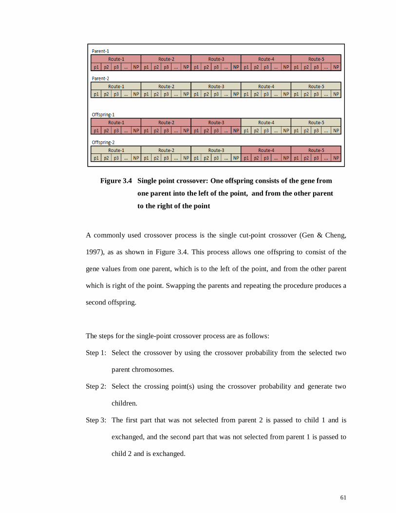
61

Figure 3.4 Single point crossover: One offspring consists of the gene from

one parent into the left of the point, and from the other parent

to the right of the point

A commonly used crossover process is the single cut-point crossover (Gen & Cheng,

1997), as as shown in Figure 3.4. This process allows one offspring to consist of the

gene values from one parent, which is to the left of the point, and from the other parent

which is right of the point. Swapping the parents and repeating the procedure produces a

second offspring.

The steps for the single-point crossover process are as follows:

Step 1: Select the crossover by using the crossover probability from the selected two

parent chromosomes.

Step 2: Select the crossing point(s) using the crossover probability and generate two

children.

Step 3: The first part that was not selected from parent 2 is passed to child 1 and is

exchanged, and the second part that was not selected from parent 1 is passed to

child 2 and is exchanged.

62

F. Mutation

Mutation is another genetic operation which provides diversity for the solutions so as to

prevent them from falling into local optima. The mutation process produces genes that

are more capable of keeping the chromosomes in the selection process and it is expected

to produce a more optimal solution. The gene mutations that result in the least fit

chromosomes are eliminated in the selection process.

Whether a gene is selected or not is determined by the mutation rate (Pm). If the

probability of mutation is low, then a possibly useful gene is noticed but should not be

selected. Conversely, if the probability of mutation is high, then the offspring might lose

the characteristics of its parents. This process results in the Genetic Algorithm losing the

ability to learn in the process of finding the optimal solution (Gen & Cheng, 1997). The

process of gene selection replaces missing genes from the population caused by the

selection process, and enables the re-emergence of genes that do not appear in the initial

population. The selection process randomly selects genes to be altered. The number of

selected genes depends on the probability of a predetermined mutation rate.

Point mutation was applied to vehicle allocations in Jeon et al. (2007). The steps for

point mutation are as follows:

Step 1: Select a gene randomly for mutation.

Step 2: Change the vehicle number randomly.

G. Genetic Algorithm Parameters

The parameters of the Genetic Algorithm consist of the population size, the number of

iterations, and the value of the mutation and crossover rates. Nothing definite is

specified regarding the parameters of a Genetic Algorithm that is used to solve all

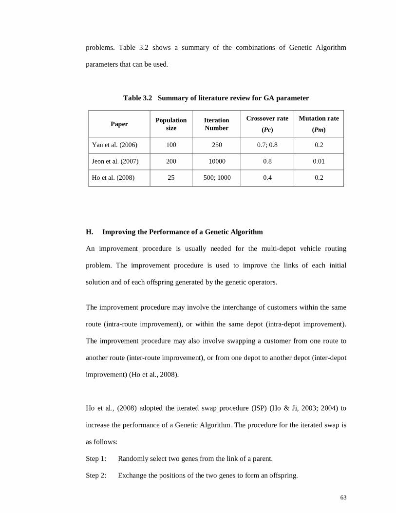
63

problems. Table 3.2 shows a summary of the combinations of Genetic Algorithm

parameters that can be used.

Table 3.2 Summary of literature review for GA parameter

Paper Population size

Iteration Number

Crossover rate

(Pc)

Mutation rate

(Pm)

Yan et al. (2006) 100 250 0.7; 0.8 0.2

Jeon et al. (2007) 200 10000 0.8 0.01

Ho et al. (2008) 25 500; 1000 0.4 0.2

H. Improving the Performance of a Genetic Algorithm

An improvement procedure is usually needed for the multi-depot vehicle routing

problem. The improvement procedure is used to improve the links of each initial

solution and of each offspring generated by the genetic operators.

The improvement procedure may involve the interchange of customers within the same

route (intra-route improvement), or within the same depot (intra-depot improvement).

The improvement procedure may also involve swapping a customer from one route to

another route (inter-route improvement), or from one depot to another depot (inter-depot

improvement) (Ho et al., 2008).

Ho et al., (2008) adopted the iterated swap procedure (ISP) (Ho & Ji, 2003; 2004) to

increase the performance of a Genetic Algorithm. The procedure for the iterated swap is

as follows:

Step 1: Randomly select two genes from the link of a parent.

Step 2: Exchange the positions of the two genes to form an offspring.

64

Step 3: Swap the neighbours of the two genes to form four more offspring.

Step 4: Evaluate all the offspring to find the best one.

Step 5: If the best offspring is better than a parent, replace the parent with the best

offspring and go back to Step 1. Otherwise, discontinue the process.

3.7 Summary

This chapter reviewed some variants of the vehicle routing problem i.e. the multi-depot

vehicle routing problem (MDVRP), the heterogeneous fleet vehicle routing problem

(HVRP), the site-dependent capacitated vehicle routing problem (SDCVRP), and the

asymmetric vehicle routing problem (AVRP). A summary of the literature that was

reviewed in relation to the problems and the methods used to solve the problems is given

in Table 3.3.

The discussion shows that there is no method that combines all four vehicle routing

problem variants that are similar to the problem to be solved. The case studies have

subject goals for accessibility and profitability. Thus, combining a fourth vehicle routing

problem variant with goals should be considered, one that is not limited to a minimum

travel distance, minimum cost or maximum profit.

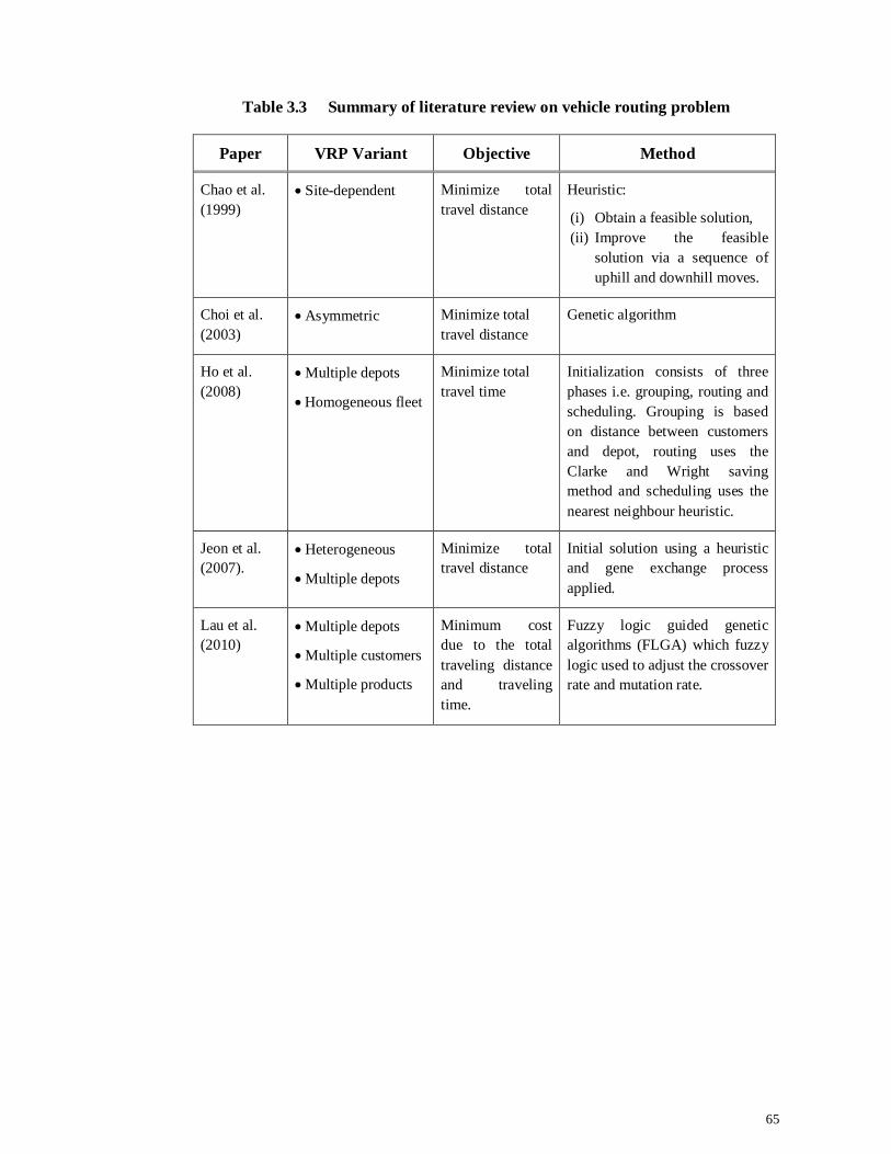
65

Table 3.3 Summary of literature review on vehicle routing problem

Paper VRP Variant Objective Method

Chao et al. (1999)

Site-dependent Minimize total travel distance

Heuristic:

(i) Obtain a feasible solution, (ii) Improve the feasible

solution via a sequence of uphill and downhill moves.

Choi et al. (2003)

Asymmetric Minimize total travel distance

Genetic algorithm

Ho et al. (2008)

Multiple depots

Homogeneous fleet

Minimize total travel time

Initialization consists of three phases i.e. grouping, routing and scheduling. Grouping is based on distance between customers and depot, routing uses the Clarke and Wright saving method and scheduling uses the nearest neighbour heuristic.

Jeon et al. (2007).

Heterogeneous

Multiple depots

Minimize total travel distance

Initial solution using a heuristic and gene exchange process applied.

Lau et al. (2010)

Multiple depots

Multiple customers

Multiple products

Minimum cost due to the total traveling distance and traveling time.

Fuzzy logic guided genetic algorithms (FLGA) which fuzzy logic used to adjust the crossover rate and mutation rate.

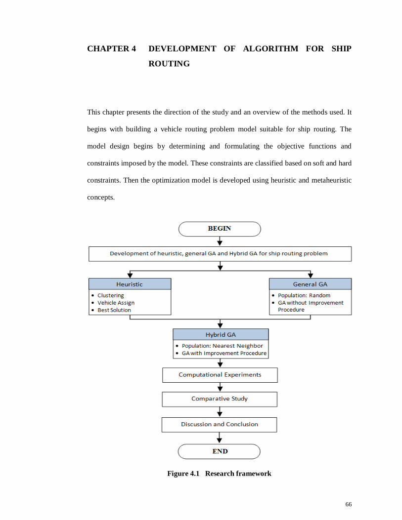
66

CHAPTER 4 DEVELOPMENT OF ALGORITHM FOR SHIP

ROUTING

This chapter presents the direction of the study and an overview of the methods used. It

begins with building a vehicle routing problem model suitable for ship routing. The

model design begins by determining and formulating the objective functions and

constraints imposed by the model. These constraints are classified based on soft and hard

constraints. Then the optimization model is developed using heuristic and metaheuristic

concepts.

Figure 4.1 Research framework

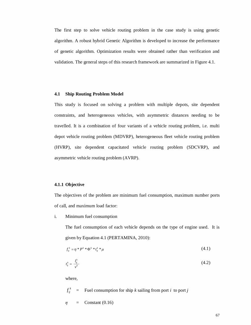
67

The first step to solve vehicle routing problem in the case study is using genetic

algorithm. A robust hybrid Genetic Algorithm is developed to increase the performance

of genetic algorithm. Optimization results were obtained rather than verification and

validation. The general steps of this research framework are summarized in Figure 4.1.

4.1 Ship Routing Problem Model

This study is focused on solving a problem with multiple depots, site dependent

constraints, and heterogeneous vehicles, with asymmetric distances needing to be

travelled. It is a combination of four variants of a vehicle routing problem, i.e. multi

depot vehicle routing problem (MDVRP), heterogeneous fleet vehicle routing problem

(HVRP), site dependent capacitated vehicle routing problem (SDCVRP), and

asymmetric vehicle routing problem (AVRP).

4.1.1 Objective

The objectives of the problem are minimum fuel consumption, maximum number ports

of call, and maximum load factor:

i. Minimum fuel consumption

The fuel consumption of each vehicle depends on the type of engine used. It is

given by Equation 4.1 (PERTAMINA, 2010):

**** kij

kkkij tPf (4.1)

k

kijk

ij vl

t

(4.2)

where,

kijf = Fuel consumption for ship k sailing from port i to port j

η = Constant (0.16)

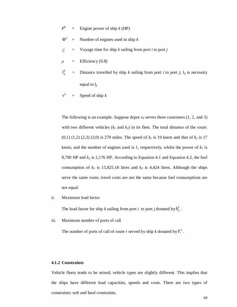
68

Pk = Engine power of ship k (HP)

k = Number of engines used in ship k

kijt = Voyage time for ship k sailing from port i to port j

μ = Efficiency (0.8)

kijl = Distance travelled by ship k sailing from port i to port j; lij is necessity

equal to lji

kv = Speed of ship k

The following is an example. Suppose depot v0 serves three customers (1, 2, and 3)

with two different vehicles (k1 and k2) in its fleet. The total distance of the route:

(0,1) (1,2) (2,3) (3,0) is 270 miles. The speed of k1 is 19 knots and that of k2 is 17

knots, and the number of engines used is 1, respectively, whilst the power of k1 is

8,700 HP and k2 is 2,176 HP. According to Equation 4.1 and Equation 4.2, the fuel

consumption of k1 is 15,825.18 litres and k2 is 4,424 litres. Although the ships

serve the same route, travel costs are not the same because fuel consumptions are

not equal.

ii. Maximum load factor

The load factor for ship k sailing from port i to port j donated by kijb .

iii. Maximum number of ports of call

The number of ports of call of route r served by ship k donated by krY .

4.1.2 Constraints

Vehicle fleets tends to be mixed; vehicle types are slightly different. This implies that

the ships have different load capacities, speeds and costs. There are two types of

constraints: soft and hard constraints.

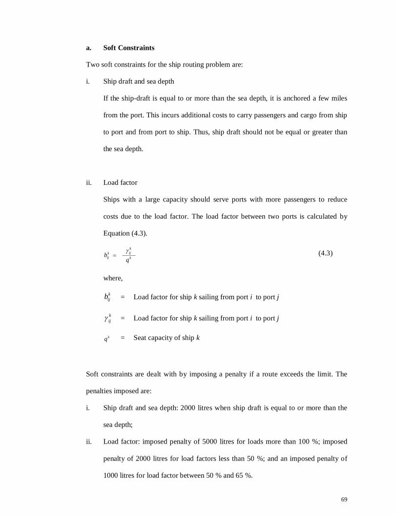
69

a. Soft Constraints

Two soft constraints for the ship routing problem are:

i. Ship draft and sea depth

If the ship-draft is equal to or more than the sea depth, it is anchored a few miles

from the port. This incurs additional costs to carry passengers and cargo from ship

to port and from port to ship. Thus, ship draft should not be equal or greater than

the sea depth.

ii. Load factor

Ships with a large capacity should serve ports with more passengers to reduce

costs due to the load factor. The load factor between two ports is calculated by

Equation (4.3).

k

kijk

ij qb

(4.3)

where,

kijb = Load factor for ship k sailing from port i to port j

kij = Load factor for ship k sailing from port i to port j

kq = Seat capacity of ship k

Soft constraints are dealt with by imposing a penalty if a route exceeds the limit. The

penalties imposed are:

i. Ship draft and sea depth: 2000 litres when ship draft is equal to or more than the

sea depth;

ii. Load factor: imposed penalty of 5000 litres for loads more than 100 %; imposed

penalty of 2000 litres for load factors less than 50 %; and an imposed penalty of

1000 litres for load factor between 50 % and 65 %.

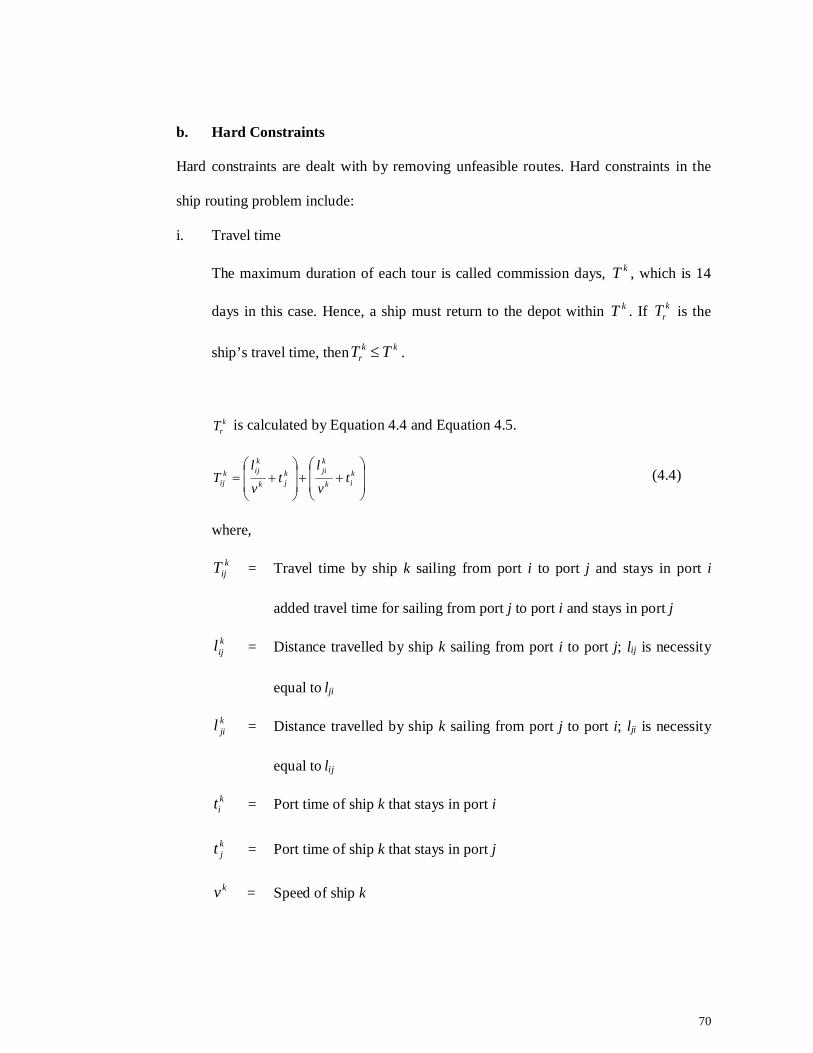
70

b. Hard Constraints

Hard constraints are dealt with by removing unfeasible routes. Hard constraints in the

ship routing problem include:

i. Travel time

The maximum duration of each tour is called commission days, kT , which is 14

days in this case. Hence, a ship must return to the depot within kT . If krT is the

ship’s travel time, then kkr TT .

krT is calculated by Equation 4.4 and Equation 4.5.

k

ik

kjik

jk

kijk

ij tv

lt

v

lT (4.4)

where,

kijT = Travel time by ship k sailing from port i to port j and stays in port i

added travel time for sailing from port j to port i and stays in port j

kijl = Distance travelled by ship k sailing from port i to port j; lij is necessity

equal to lji

kjil = Distance travelled by ship k sailing from port j to port i; lji is necessity

equal to lij

kit = Port time of ship k that stays in port i

kjt = Port time of ship k that stays in port j

kv = Speed of ship k

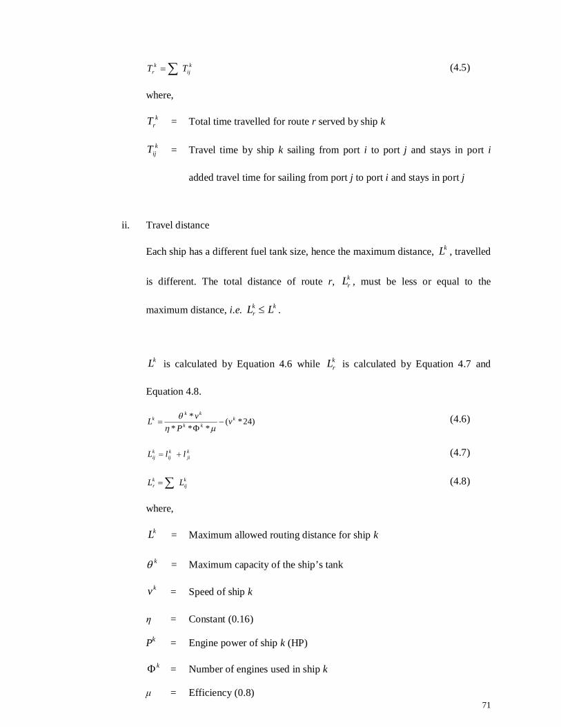
71

kij

kr TT (4.5)

where,

krT = Total time travelled for route r served by ship k

kijT = Travel time by ship k sailing from port i to port j and stays in port i

added travel time for sailing from port j to port i and stays in port j

ii. Travel distance

Each ship has a different fuel tank size, hence the maximum distance, kL , travelled

is different. The total distance of route r, krL , must be less or equal to the

maximum distance, i.e. kkr LL .

kL is calculated by Equation 4.6 while krL is calculated by Equation 4.7 and

Equation 4.8.

)24*(***

* kkk

kkk v

PvL

(4.6)

kji

kij

kij llL (4.7)

kij

kr LL (4.8)

where,

kL = Maximum allowed routing distance for ship k

k = Maximum capacity of the ship’s tank

kv = Speed of ship k

η = Constant (0.16)

Pk = Engine power of ship k (HP)

k = Number of engines used in ship k

μ = Efficiency (0.8)

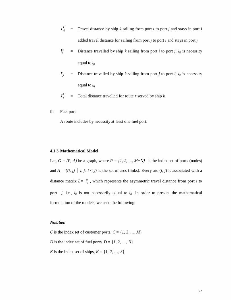
72

kijL = Travel distance by ship k sailing from port i to port j and stays in port i

added travel distance for sailing from port j to port i and stays in port j

kijl = Distance travelled by ship k sailing from port i to port j; lij is necessity

equal to lji

kjil = Distance travelled by ship k sailing from port j to port i; lji is necessity

equal to lij

krL = Total distance travelled for route r served by ship k

iii. Fuel port

A route includes by necessity at least one fuel port.

4.1.3 Mathematical Model

Let, G = (P, A) be a graph, where P = {1, 2, ..., M+N} is the index set of ports (nodes)

and A = {(i, j) │ i, j; i < j} is the set of arcs (links). Every arc (i, j) is associated with a

distance matrix L= kijl , which represents the asymmetric travel distance from port i to

port j, i.e., lij is not necessarily equal to lji. In order to present the mathematical

formulation of the models, we used the following:

Notation

C is the index set of customer ports, C = {1, 2, …, M}

D is the index set of fuel ports, D = {1, 2, …, N}

K is the index set of ships, K = {1, 2, …, S}

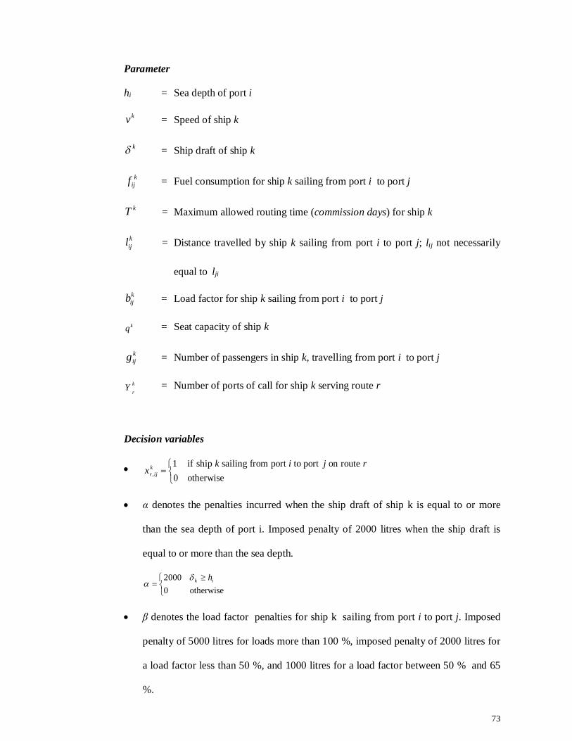
73

Parameter

hi = Sea depth of port i

kv = Speed of ship k

k = Ship draft of ship k

kijf = Fuel consumption for ship k sailing from port i to port j

kT = Maximum allowed routing time (commission days) for ship k

kijl = Distance travelled by ship k sailing from port i to port j; lij not necessarily

equal to lji

kijb = Load factor for ship k sailing from port i to port j

kq = Seat capacity of ship k

kijg = Number of passengers in ship k, travelling from port i to port j

k

rY = Number of ports of call for ship k serving route r

Decision variables

otherwise0

routeon port toport from sailing ship if1,

rj ikx k

ijr

α denotes the penalties incurred when the ship draft of ship k is equal to or more

than the sea depth of port i. Imposed penalty of 2000 litres when the ship draft is

equal to or more than the sea depth.

otherwise0

2000 ik h

β denotes the load factor penalties for ship k sailing from port i to port j. Imposed

penalty of 5000 litres for loads more than 100 %, imposed penalty of 2000 litres for

a load factor less than 50 %, and 1000 litres for a load factor between 50 % and 65

%.

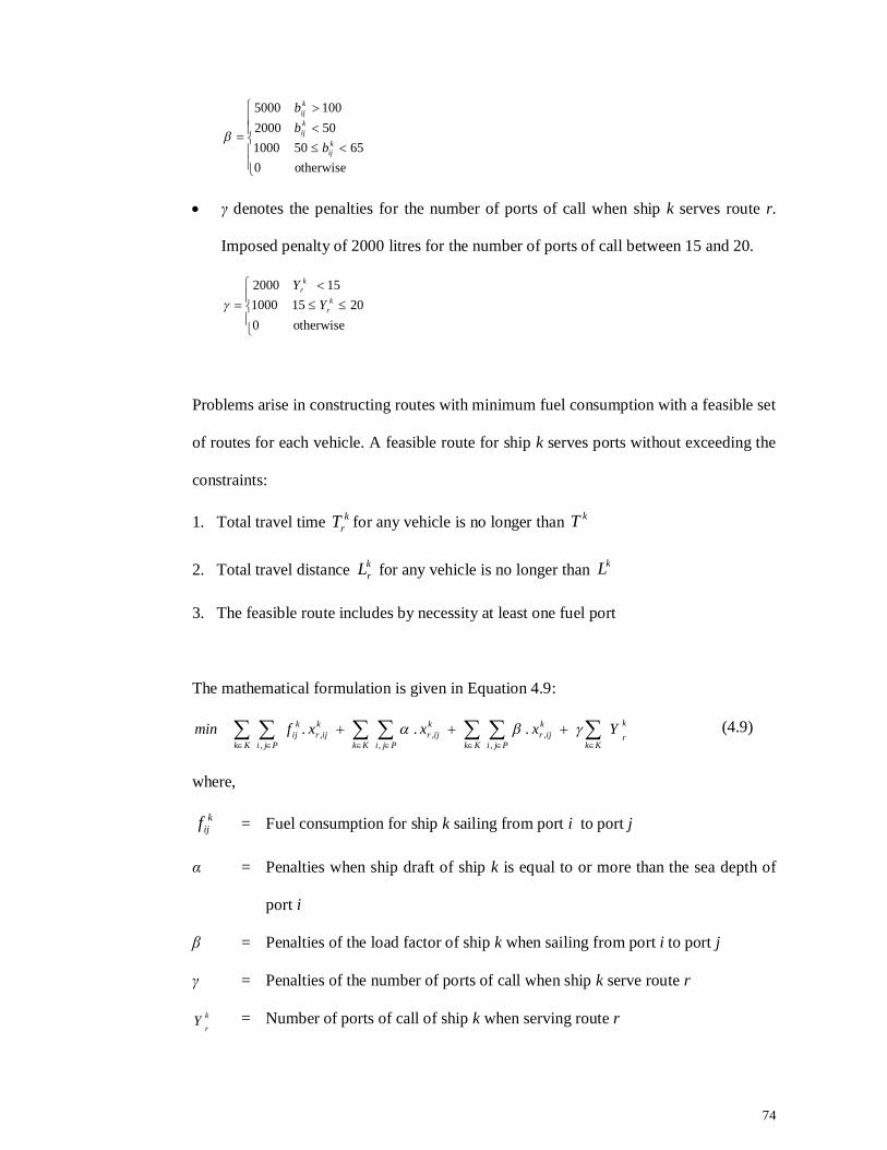
74

otherwise065501000

5020001005000

kij

kij

kij

bbb

γ denotes the penalties for the number of ports of call when ship k serves route r.

Imposed penalty of 2000 litres for the number of ports of call between 15 and 20.

otherwise0

20151000152000k

r

kr

YY

Problems arise in constructing routes with minimum fuel consumption with a feasible set

of routes for each vehicle. A feasible route for ship k serves ports without exceeding the

constraints:

1. Total travel time krT for any vehicle is no longer than kT

2. Total travel distance krL for any vehicle is no longer than kL

3. The feasible route includes by necessity at least one fuel port

The mathematical formulation is given in Equation 4.9:

k

rKkKk

kijr

PjiKk

kijr

PjiKk

kijr

kij

PjiYxxxfmin

. . . ,,

,,

,,

(4.9)

where,

kijf = Fuel consumption for ship k sailing from port i to port j

α = Penalties when ship draft of ship k is equal to or more than the sea depth of

port i

β = Penalties of the load factor of ship k when sailing from port i to port j

γ = Penalties of the number of ports of call when ship k serve route r

k

rY = Number of ports of call of ship k when serving route r

75

The objectives is to minimize total fuel consumption on routes travelled, the penalty cost

for violations of the ship draft and sea depth, the penalty cost for violations of the load

factor, and the penalty cost for violations of the number of ports of call.

Subject to:

1. All ports (customer and fuel ports) i are serviced by ship k at least once.

2. Travel time of ship k is no longer than the maximum allowed routing time kT .

3. Total distance travelled for route r served by ship k is no longer than the maximum

allowed routing distance of ship k.

4. Ship draft of ship k must be less than the sea depth of port i.

5. Route r served by ship k should possess a fuel-port.

The feasible route combination should meet the requirements:

Each route is served by one ship

Each port is served at least once

Each route has at least one fuel port

Each ship has a total travel time within 14 days

Each ship does not exceed the allowed travel distance

4.2 Heuristic Method

This study uses a heuristic method ‘cluster first and route second’ (Gillett & Miller,

1974), adopted for solving four VRP variants. The method involves three phases;

clustering, assigning of vehicles, and finding the best routes by combining feasible

solutions.

76

4.2.1 Heuristic for Ship Routing Problem

The three phases of the algorithm are:

(i) Phase I: Clustering

Routes are clustered to solve the problem based on the constraints of travel time

and travel distance allowed for each route. Travel time is less than or equal to the

maximum travel time allowed, and the travel distance is less than or equal to the

maximum travel distance allowed. The output is a feasible route set for the

solution candidate. Process for clustering shows in flowchart, Figure 4.2.

(ii) Phase II: Assigning Vehicle

Vehicles are assigned in a cluster to ensure each route has at least one fuel port. A

route is removed if this condition is violated. In this phase, fuel consumption is

calculated with penalty α imposed if the ship’s draft is equal to or greater than the

sea depth, penalty β for the load factor conditions, and penalty γ for the number of

ports of call. Assigning vehicle processes shown in flowchart, Figure 4.3.

(iii) Phase III: Finding Best Routes

A robust algorithm was developed based on the maximum-insertion concept

(Pertiwi, 2005). The heuristic model with the maximum-insertion concept is

modified with the idea of successively inserting a route into the best combination

of routes with minimum fuel consumption. Finding best routes processes shown in

flowchart, Figure 4.4.

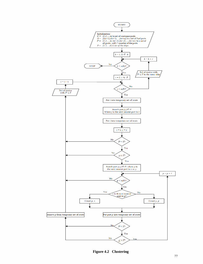
77

Figure 4.2 Clustering

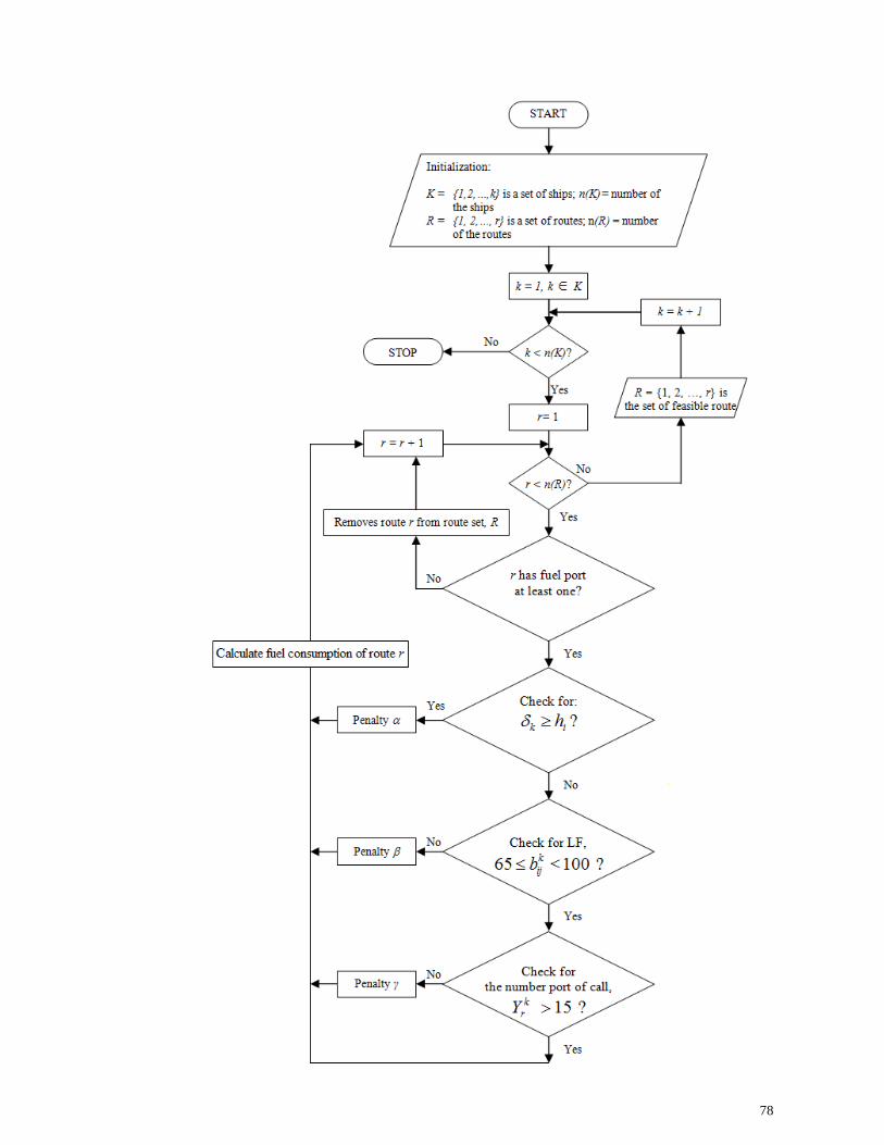
78

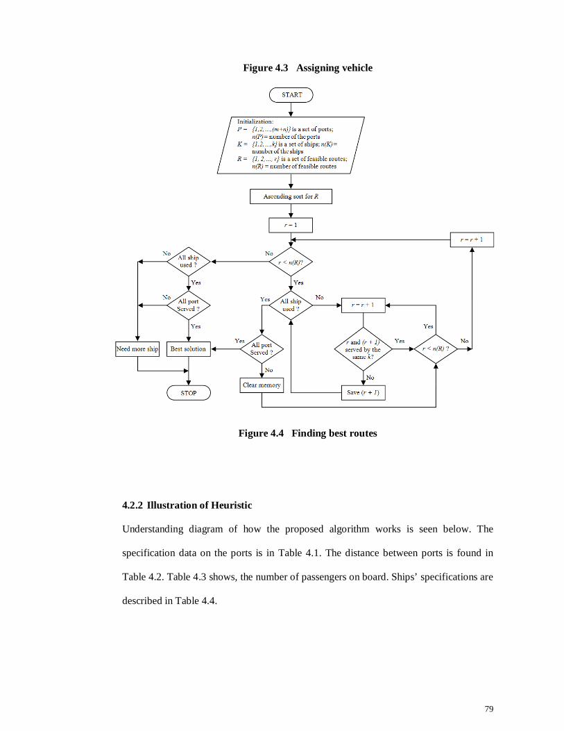
79

Figure 4.3 Assigning vehicle

Figure 4.4 Finding best routes

4.2.2 Illustration of Heuristic

Understanding diagram of how the proposed algorithm works is seen below. The

specification data on the ports is in Table 4.1. The distance between ports is found in

Table 4.2. Table 4.3 shows, the number of passengers on board. Ships’ specifications are

described in Table 4.4.

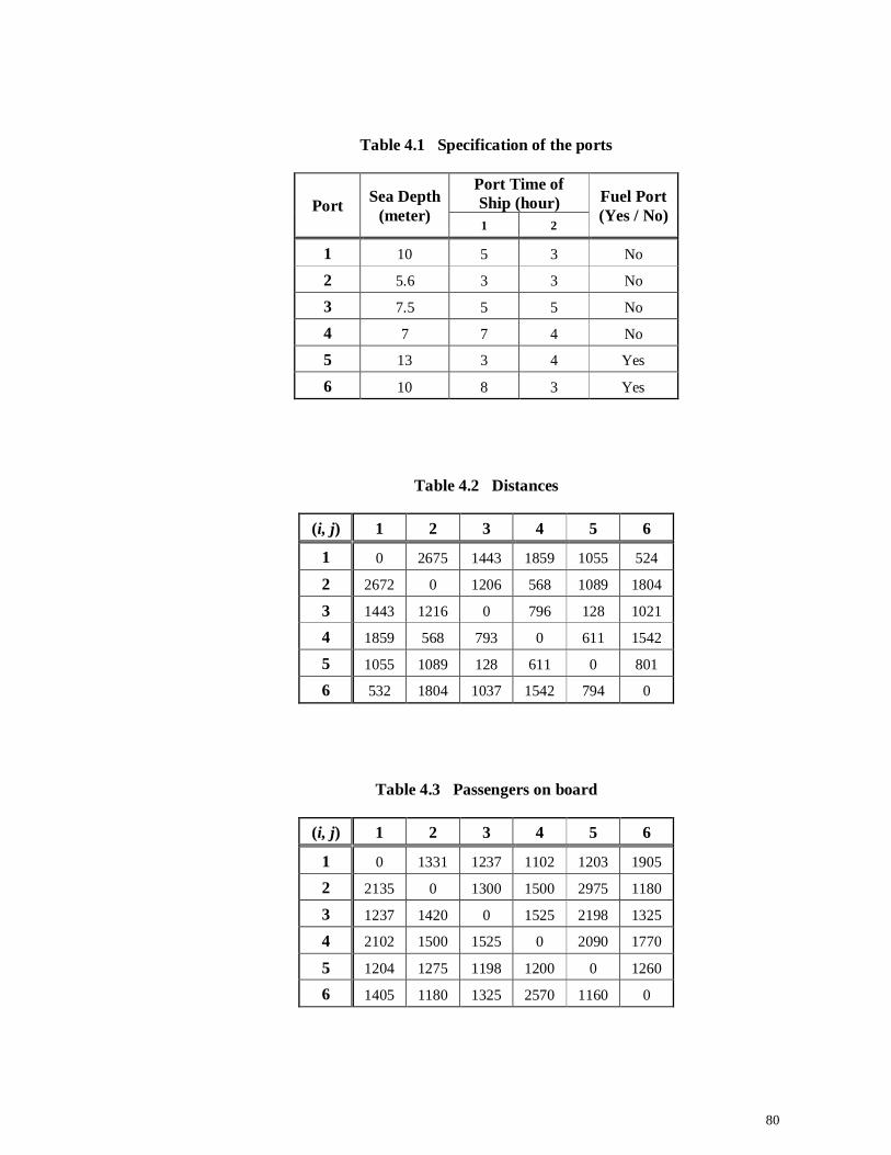
80

Table 4.1 Specification of the ports

Port Sea Depth (meter)

Port Time of Ship (hour) Fuel Port

(Yes / No) 1 2

1 10 5 3 No

2 5.6 3 3 No

3 7.5 5 5 No

4 7 7 4 No

5 13 3 4 Yes

6 10 8 3 Yes

Table 4.2 Distances

(i, j) 1 2 3 4 5 6

1 0 2675 1443 1859 1055 524

2 2672 0 1206 568 1089 1804

3 1443 1216 0 796 128 1021

4 1859 568 793 0 611 1542

5 1055 1089 128 611 0 801

6 532 1804 1037 1542 794 0

Table 4.3 Passengers on board

(i, j) 1 2 3 4 5 6

1 0 1331 1237 1102 1203 1905

2 2135 0 1300 1500 2975 1180

3 1237 1420 0 1525 2198 1325

4 2102 1500 1525 0 2090 1770

5 1204 1275 1198 1200 0 1260

6 1405 1180 1325 2570 1160 0

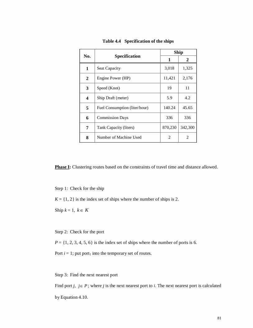
81

Table 4.4 Specification of the ships

No. Specification Ship

1 2

1 Seat Capacity 3,018 1,325

2 Engine Power (HP) 11,421 2,176

3 Speed (Knot) 19 11

4 Ship Draft (meter) 5.9 4.2

5 Fuel Consumption (liter/hour) 140.24 45.65

6 Commission Days 336 336

7 Tank Capacity (liters) 870,230 342,300

8 Number of Machine Used 2 2

Phase I: Clustering routes based on the constraints of travel time and distance allowed.

Step 1: Check for the ship

K = {1, 2} is the index set of ships where the number of ships is 2.

Ship k = 1, Kk

Step 2: Check for the port

P = {1, 2, 3, 4, 5, 6} is the index set of ships where the number of ports is 6.

Port i = 1; put port1 into the temporary set of routes.

Step 3: Find the next nearest port

Find port j, Pj ; where j is the next nearest port to i. The next nearest port is calculated

by Equation 4.10.

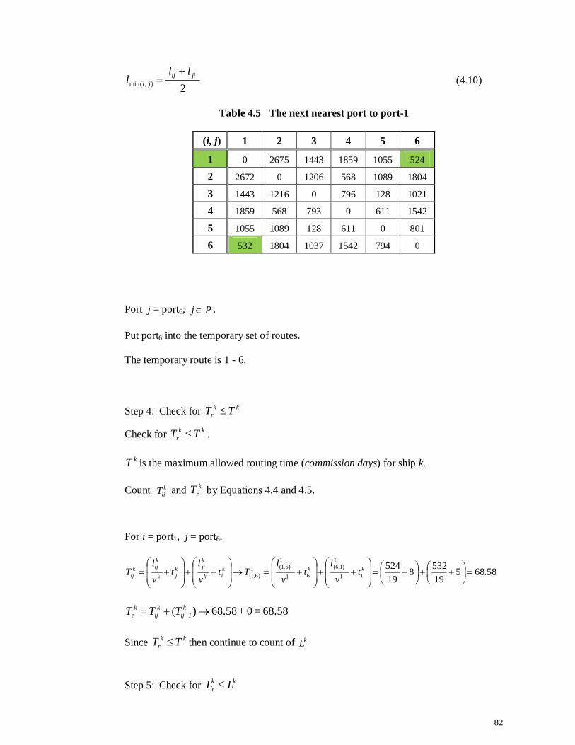
82

2

) ,(minjiij

ji

lll

(4.10)

Table 4.5 The next nearest port to port-1

(i, j) 1 2 3 4 5 6

1 0 2675 1443 1859 1055 524

2 2672 0 1206 568 1089 1804

3 1443 1216 0 796 128 1021

4 1859 568 793 0 611 1542

5 1055 1089 128 611 0 801

6 532 1804 1037 1542 794 0

Port j = port6; Pj .

Put port6 into the temporary set of routes.

The temporary route is 1 - 6.

Step 4: Check for kkr TT

Check for kkr TT .

kT is the maximum allowed routing time (commission days) for ship k.

Count kijT and k

rT by Equations 4.4 and 4.5.

For i = port1, j = port6.

58.685195328

19524

11

1)1,6(

61

1)6,1(1

)6,1(

kkk

ik

kjik

jk

kijk

ij tv

lt

v

lTt

v

lt

v

lT

68.58 = 0 + 68.58)(r k

1ijk

ijk TTT

Since kkr TT then continue to count of kL

Step 5: Check for kk

r LL

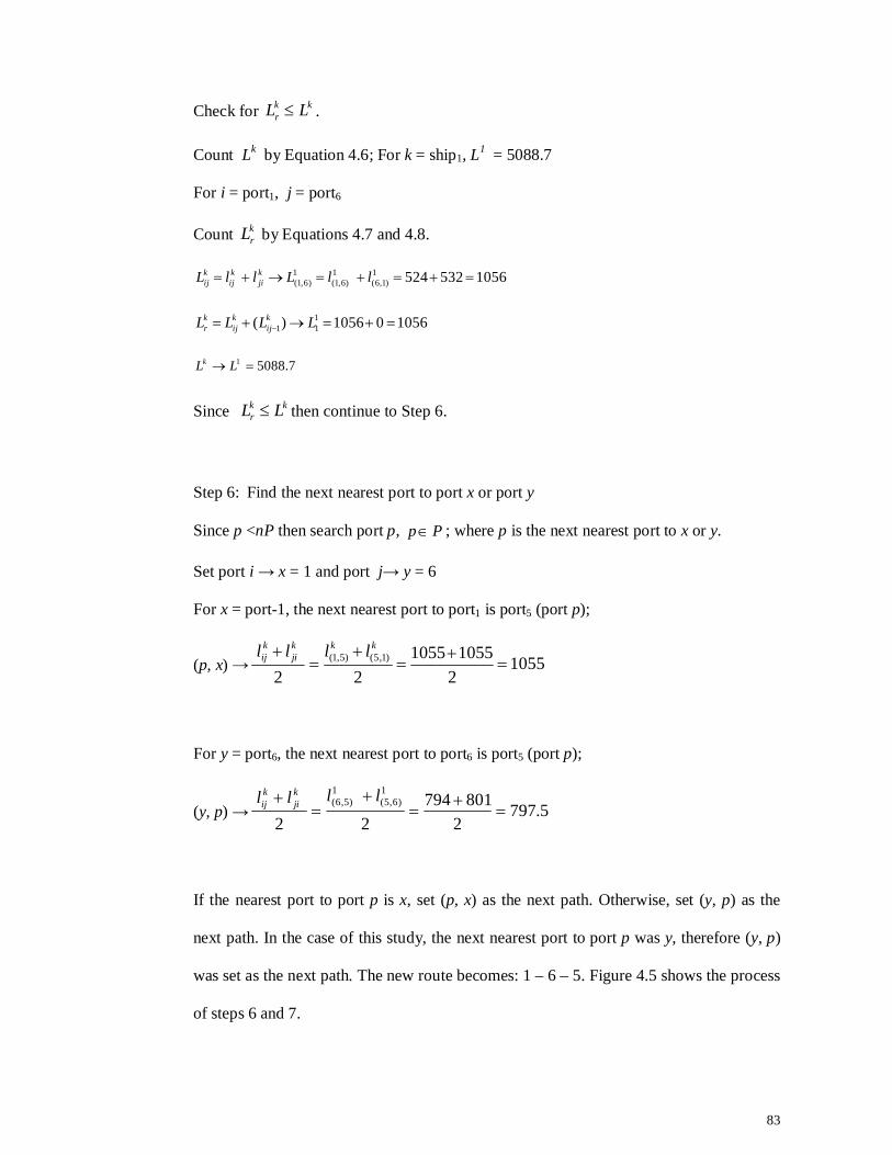
83

Check for kkr LL .

Count Lk by Equation 4.6; For k = ship1, L1 = 5088.7

For i = port1, j = port6

Count krL by Equations 4.7 and 4.8.

10565325241)1,6(

1)6,1(

1)6,1( llLllL k

jikij

kij

105601056)( 111 LLLL k

ijkij

kr

7.50881 LLk

Since kkr LL then continue to Step 6.

Step 6: Find the next nearest port to port x or port y

Since p <nP then search port p, Pp ; where p is the next nearest port to x or y.

Set port i → x = 1 and port j→ y = 6

For x = port-1, the next nearest port to port1 is port5 (port p);

(p, x) → 10552

1055105522

)1,5()5,1(

kkk

jikij llll

For y = port6, the next nearest port to port6 is port5 (port p);

(y, p) → 5.7972

80179422

1)6,5(

1)5,6(

llll k

jikij

If the nearest port to port p is x, set (p, x) as the next path. Otherwise, set (y, p) as the

next path. In the case of this study, the next nearest port to port p was y, therefore (y, p)

was set as the next path. The new route becomes: 1 – 6 – 5. Figure 4.5 shows the process

of steps 6 and 7.

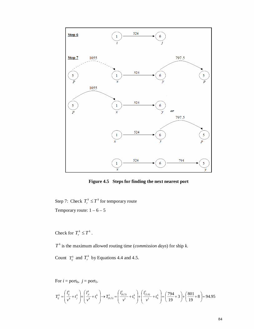
84

Figure 4.5 Steps for finding the next nearest port

Step 7: Check kkr TT for temporary route

Temporary route: 1 – 6 – 5

Check for kkr TT .

kT is the maximum allowed routing time (commission days) for ship k.

Count kijT and k

rT by Equations 4.4 and 4.5.

For i = port6, j = port5.

95.948198013

19794

61

1)6,5(

51

1)5,6(1

)5,6(

kkk

ik

kjik

jk

kijk

ij tv

lt

vl

Ttvl

tvl

T

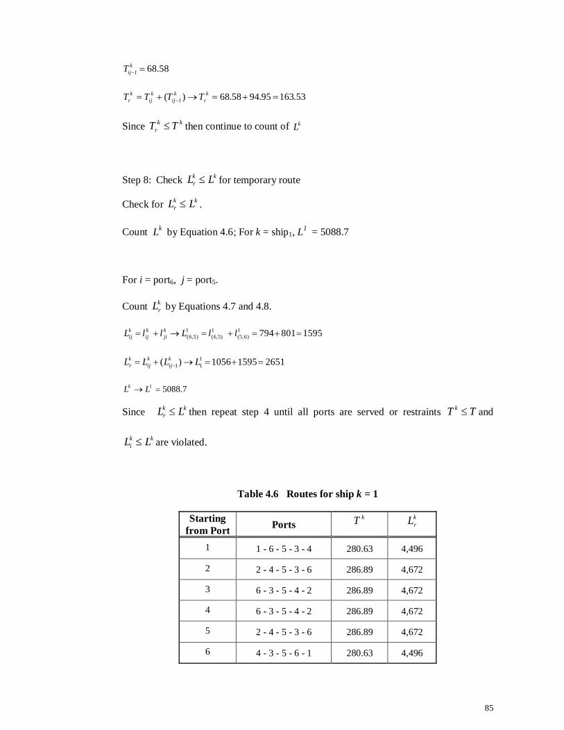
85

68.58k

1ijT

53.16395.9458.68)( k

rk

1ijk

ijk

r TTTT

Since kkr TT then continue to count of kL

Step 8: Check kkr LL for temporary route

Check for kkr LL .

Count Lk by Equation 4.6; For k = ship1, L1 = 5088.7

For i = port6, j = port5.

Count krL by Equations 4.7 and 4.8.

15958017941)6,5(

1)5,6(

1)5,6( llLllL k

jikij

kij

265115951056)( 111 LLLL k

ijkij

kr

7.50881 LLk

Since kkr LL then repeat step 4 until all ports are served or restraints TT k and

kki LL are violated.

Table 4.6 Routes for ship k = 1

Starting from Port Ports

kT krL

1 1 - 6 - 5 - 3 - 4 280.63 4,496

2 2 - 4 - 5 - 3 - 6 286.89 4,672

3 6 - 3 - 5 - 4 - 2 286.89 4,672

4 6 - 3 - 5 - 4 - 2 286.89 4,672

5 2 - 4 - 5 - 3 - 6 286.89 4,672

6 4 - 3 - 5 - 6 - 1 280.63 4,496

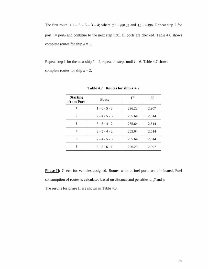
86

The first route is 1 – 6 – 5 – 3 – 4; where 63.280kT and 496,4krL . Repeat step 2 for

port i = port2 and continue to the next step until all ports are checked. Table 4.6 shows

complete routes for ship k = 1.

Repeat step 1 for the next ship k = 2, repeat all steps until i = 6. Table 4.7 shows

complete routes for ship k = 2.

Table 4.7 Routes for ship k = 2

Starting from Port Ports

kT krL

1 1 - 6 - 5 - 3 296.23 2,907

2 2 - 4 - 5 - 3 265.64 2,614

3 3 - 5 - 4 - 2 265.64 2,614

4 3 - 5 - 4 - 2 265.64 2,614

5 2 - 4 - 5 - 3 265.64 2,614

6 3 - 5 - 6 - 1 296.23 2,907

Phase II: Check for vehicles assigned. Routes without fuel ports are eliminated. Fuel

consumption of routes is calculated based on distance and penalties α, β and γ.

The results for phase II are shown in Table 4.8.

87

Table 4.8 Output of phase II

88

Phase III: Finding the best combination of routes.

The best combination of routes with minimum fuel consumption and maximal ports of

call is found using the ‘maximum-insertion concept’ (Pertiwi, 2005).

Step 1: Ascending routes

Sort all routes based on fuel consumption, as shown in Table 4.9.

89

Table 4.9 Sort all routes based on fuel consumption

90

Step 2: Check the best route for the first ship

R = {1, 2, ..., 12} is an index set of the routes, where the number of routes is 12.

Check for first route r = 8.

Save r = 8 into temporary best solution.

Step 3: Check the best route for the second ship

Check for the next route, r = 9.

Identification of ship and port served. If route r = 8 and r = 9 are served by the same ship

then continue to search for the next route.

Check for the 7th route, r = 1; r < nR.

Identification of ship and port served. If route r = 1 is served by a different ship then

save route r = 1 into temporary best solution. Check ports served; if all ports are served

then it is chosen as the best combination, otherwise, the temporary solution is cleared

and continues to check for the next route.

Since route r = 8 and r = 1 are served by different ships and all ports are served then it is

chosen as the best combination route.

Ship k = 1 serves route r = 1 (ports: 1 – 6 – 5 – 3 – 4)

Fuel consumption = 824,004 litres

Average of load factor = 121%

Number of ports of call = 9 (ports: 1 – 6 – 5 – 3 – 4 – 3 – 5 – 6 – 1)

Ship k = 2 serves route r = 8 (ports: 2 – 4 – 5 – 3 – 5 – 4 – 2)

Fuel consumption = 163,976 litres

Average of load factor = 51%

Number of ports of call = 7

91

4.3 Genetic Algorithm

A general Genetic Algorithm (Gen & Cheng, 1999) can be represented by following

these major steps:

Step 1: Represent the problem as a chromosome; choose the population size, the

crossover rate and the mutation rate.

Step 2: Define a fitness function to measure the performance, or fitness, of an

individual chromosome in the problem domain.

Step 3: Randomly generate chromosomes in a population of size, pop_size.

Step 4: Calculate fitness values.

Step 5: Select chromosomes from the current population.

Step 6: Create offspring by using crossover and mutation.

Step 7: Place the created offspring chromosomes into a new population.

Step 8: Repeat step 5 until the number of chromosomes equals to the population size.

Step 9: Replace the parent with the new population (offspring).

Step 10: Return to step 4, and repeat the process until termination criteria are satisfied.

4.3.1 Genetic Algorithm for a Ship Routing Problem

Representing chromosomes is the first step in Genetic Algorithm. This is followed by

generate chromosomes in the first generating, evaluating fitness values, selection,

crossover, and mutation. The processes are depicted in Figure 4.6.

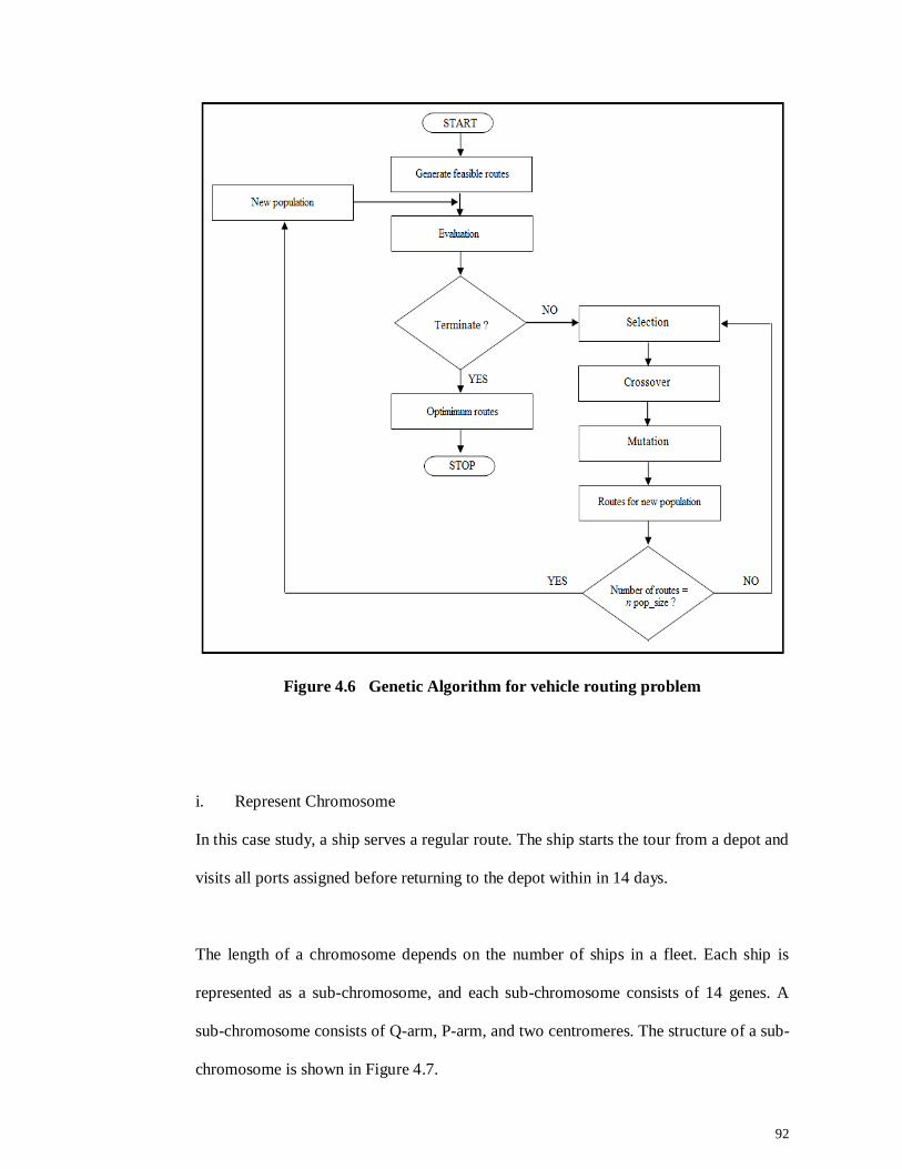
92

Figure 4.6 Genetic Algorithm for vehicle routing problem

i. Represent Chromosome

In this case study, a ship serves a regular route. The ship starts the tour from a depot and

visits all ports assigned before returning to the depot within in 14 days.

The length of a chromosome depends on the number of ships in a fleet. Each ship is

represented as a sub-chromosome, and each sub-chromosome consists of 14 genes. A

sub-chromosome consists of Q-arm, P-arm, and two centromeres. The structure of a sub-

chromosome is shown in Figure 4.7.

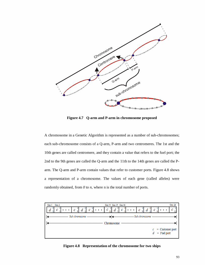
93

Figure 4.7 Q-arm and P-arm in chromosome proposed

A chromosome in a Genetic Algorithm is represented as a number of sub-chromosomes;

each sub-chromosome consists of a Q-arm, P-arm and two centromeres. The 1st and the

10th genes are called centromere, and they contain a value that refers to the fuel port; the

2nd to the 9th genes are called the Q-arm and the 11th to the 14th genes are called the P-

arm. The Q-arm and P-arm contain values that refer to customer ports. Figure 4.8 shows

a representation of a chromosome. The values of each gene (called alleles) were

randomly obtained, from 0 to n, where n is the total number of ports.

Figure 4.8 Representation of the chromosome for two ships

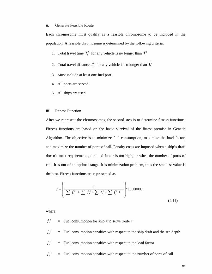
94

ii. Generate Feasible Route

Each chromosome must qualify as a feasible chromosome to be included in the

population. A feasible chromosome is determined by the following criteria:

1. Total travel time krT for any vehicle is no longer than kT

2. Total travel distance krL for any vehicle is no longer than kL

3. Must include at least one fuel port

4. All ports are served

5. All ships are used

iii. Fitness Function

After we represent the chromosomes, the second step is to determine fitness functions.

Fitness functions are based on the basic survival of the fittest premise in Genetic

Algorithm. The objective is to minimize fuel consumption, maximize the load factor,

and maximize the number of ports of call. Penalty costs are imposed when a ship’s draft

doesn’t meet requirements, the load factor is too high, or when the number of ports of

call. It is out of an optimal range. It is minimization problem, thus the smallest value is

the best. Fitness functions are represented as:

10000000* 1

1

kkkkr ffff

f

(4.11)

where,

krf = Fuel consumption for ship k to serve route r

kf = Fuel consumption penalties with respect to the ship draft and the sea depth

kbf = Fuel consumption penalties with respect to the load factor

kf = Fuel consumption penalties with respect to the number of ports of call

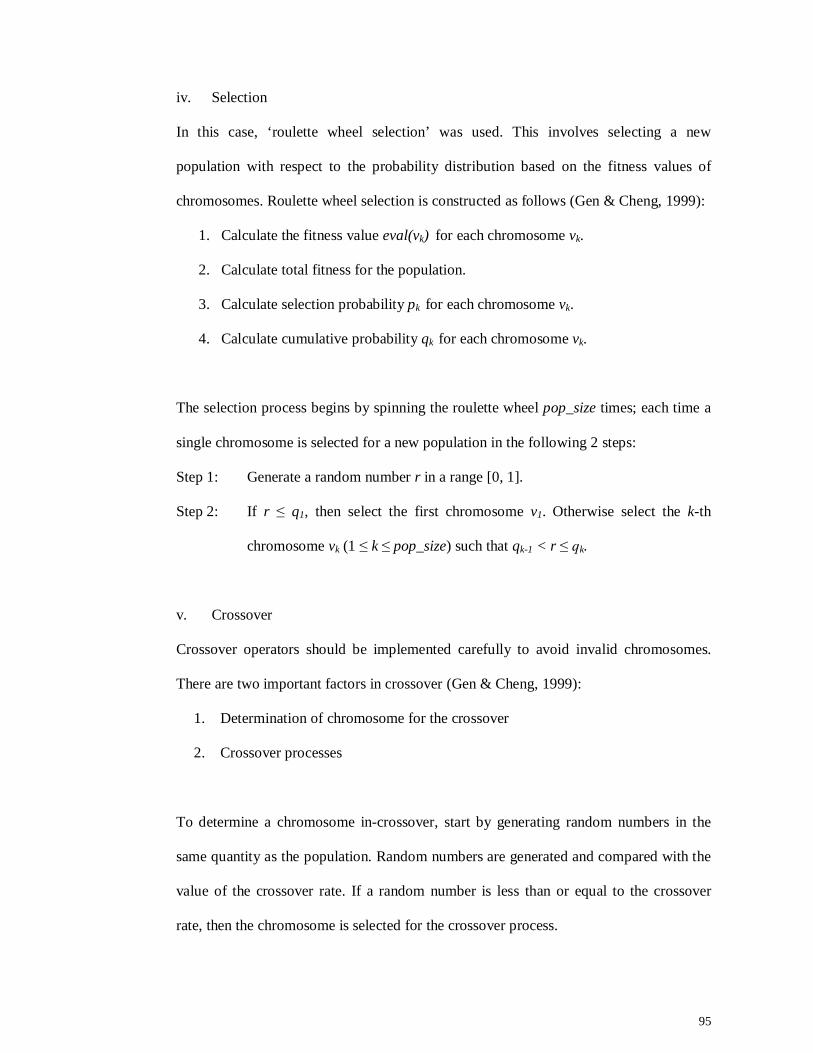
95

iv. Selection

In this case, ‘roulette wheel selection’ was used. This involves selecting a new

population with respect to the probability distribution based on the fitness values of

chromosomes. Roulette wheel selection is constructed as follows (Gen & Cheng, 1999):

1. Calculate the fitness value eval(vk) for each chromosome vk.

2. Calculate total fitness for the population.

3. Calculate selection probability pk for each chromosome vk.

4. Calculate cumulative probability qk for each chromosome vk.

The selection process begins by spinning the roulette wheel pop_size times; each time a

single chromosome is selected for a new population in the following 2 steps:

Step 1: Generate a random number r in a range [0, 1].

Step 2: If r ≤ q1, then select the first chromosome v1. Otherwise select the k-th

chromosome vk (1 ≤ k ≤ pop_size) such that qk-1 < r ≤ qk.

v. Crossover

Crossover operators should be implemented carefully to avoid invalid chromosomes.

There are two important factors in crossover (Gen & Cheng, 1999):

1. Determination of chromosome for the crossover

2. Crossover processes

To determine a chromosome in-crossover, start by generating random numbers in the

same quantity as the population. Random numbers are generated and compared with the

value of the crossover rate. If a random number is less than or equal to the crossover

rate, then the chromosome is selected for the crossover process.

96

Figure 4.9 Multi Cut Point Crossover

The process of crossover is to exchanges portions of a chromosome with another

chromosome eligible for in-crossover.

Multi cut point chromosome is applied in this research and the steps are as follow:

Step 1: Select two chromosomes eligible for in-crossover.

Step 2: Check whether the arms that are exchanged qualify as a feasible chromosome.

If the offspring violates a constraint it must be repaired.

vi. Mutation

There are two important things in mutation (Gen & Cheng, 1999):

1. Determination of chromosome for the mutation

2. Mutation processes

To determine a chromosome in-mutation, generate random numbers in the same quantity

as the population and multiple numbers of the P-arm. The random numbers are

generated and compared with the value of the mutation rate. If a random number is less

than or equal to the mutation rate, then the chromosome is selected for the mutation

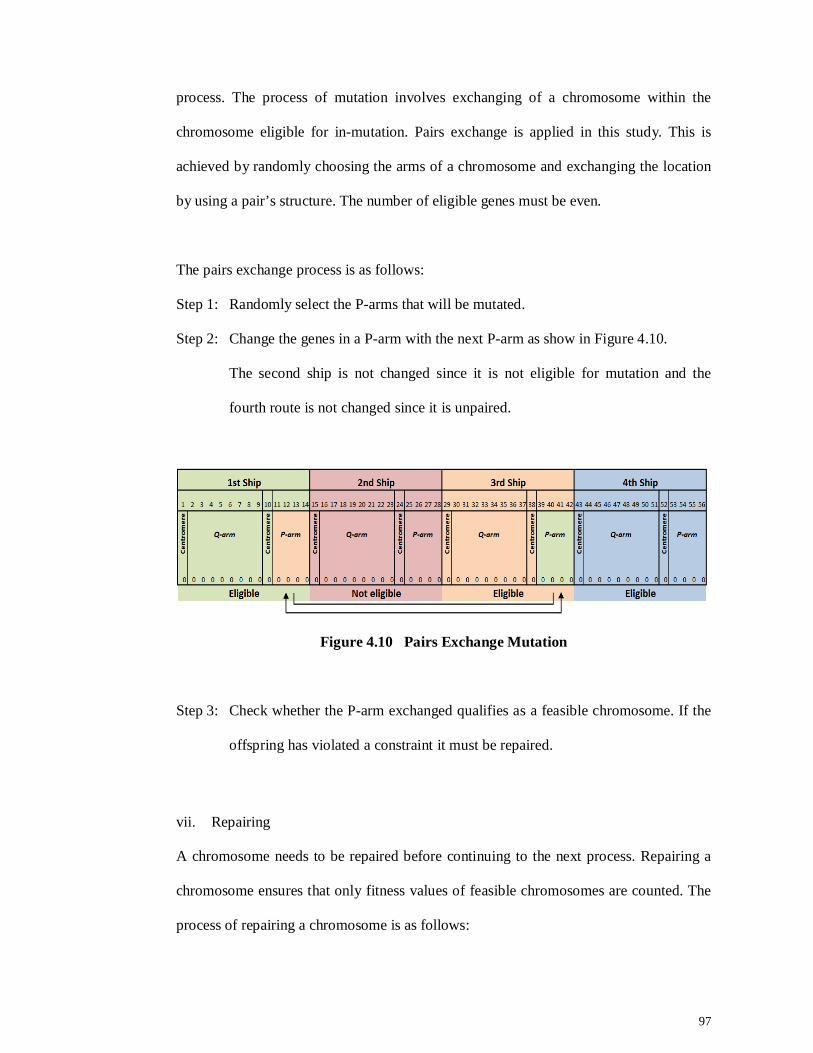
97

process. The process of mutation involves exchanging of a chromosome within the

chromosome eligible for in-mutation. Pairs exchange is applied in this study. This is

achieved by randomly choosing the arms of a chromosome and exchanging the location

by using a pair’s structure. The number of eligible genes must be even.

The pairs exchange process is as follows:

Step 1: Randomly select the P-arms that will be mutated.

Step 2: Change the genes in a P-arm with the next P-arm as show in Figure 4.10.

The second ship is not changed since it is not eligible for mutation and the

fourth route is not changed since it is unpaired.

Figure 4.10 Pairs Exchange Mutation

Step 3: Check whether the P-arm exchanged qualifies as a feasible chromosome. If the

offspring has violated a constraint it must be repaired.

vii. Repairing

A chromosome needs to be repaired before continuing to the next process. Repairing a

chromosome ensures that only fitness values of feasible chromosomes are counted. The

process of repairing a chromosome is as follows:

98

Step 1: If kkr TT and kk

r LL is violated, check the similar numbers in the same arm

and same sub-chromosome and remove them. Repeat step 1 until no similar

numbers in the same arms of the same sub-chromosome are left.

Step 2: If kkr TT and kk

r LL are violated, check the similar numbers in a different

arm but within the same sub-chromosome, and remove them. Repeat step 2

until no similar numbers in the same arm type of different sub-chromosomes

exist.

Step 3: If kkr TT and kk

r LL are violated, check the similar numbers in the same

arm and different sub-chromosome and remove them. Repeat step 3 until no

similar numbers in different arm types with the same sub-chromosome exist.

Step 4: If kkr TT and kk

r LL are violated, check the similar numbers in different

arms and different sub-chromosome and remove them.

Repeat step 4 until no similar numbers in different arm types of different sub-

chromosomes exist.

Step 5: If kkr TT and kk

r LL are still in violation, then the recombination process is

cancelled.

4.3.2 Illustration of General Genetic Algorithm

An illustration of how a general Genetic Algorithm is used for solving vehicle routing

problem is seen below. Data of specifications of the ports are seen in Table 4.1, the

distance between ports is in Table 4.2, the number of passengers on board is in Table 4.3

and the specifications of the ships are in Table 4.4.

The genetic operators used were selected by roulette wheel, crossover by multi cut point

and mutation by pairs exchange. The genetic parameters used were: population size of

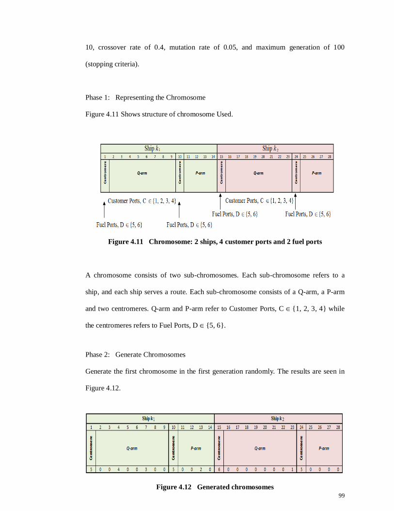
99

10, crossover rate of 0.4, mutation rate of 0.05, and maximum generation of 100

(stopping criteria).

Phase 1: Representing the Chromosome

Figure 4.11 Shows structure of chromosome Used.

Figure 4.11 Chromosome: 2 ships, 4 customer ports and 2 fuel ports

A chromosome consists of two sub-chromosomes. Each sub-chromosome refers to a

ship, and each ship serves a route. Each sub-chromosome consists of a Q-arm, a P-arm

and two centromeres. Q-arm and P-arm refer to Customer Ports, C {1, 2, 3, 4} while

the centromeres refers to Fuel Ports, D {5, 6}.

Phase 2: Generate Chromosomes

Generate the first chromosome in the first generation randomly. The results are seen in

Figure 4.12.

Figure 4.12 Generated chromosomes

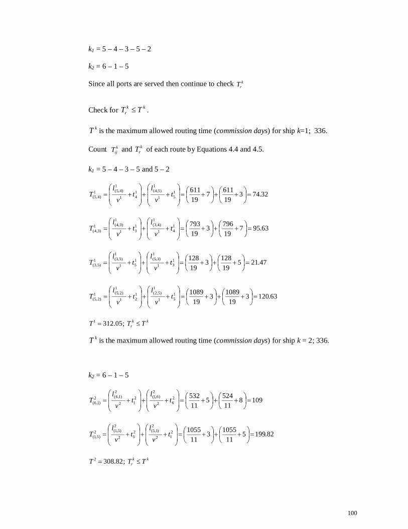
100

k1 = 5 – 4 – 3 – 5 – 2

k2 = 6 – 1 – 5

Since all ports are served then continue to check krT

Check for kk

r TT .

kT is the maximum allowed routing time (commission days) for ship k=1; 336.

Count kijT and k

rT of each route by Equations 4.4 and 4.5.

k1 = 5 – 4 – 3 – 5 and 5 – 2

32.743196117

196111

51

1)5,4(1

41

1)4,5(1

)4,5(

t

v

lt

v

lT

63.957197963

197931

41

1)4,3(1

31

1)3,4(1

)3,4(

t

v

lt

v

lT

47.215191283

191281

31

1)3,5(1

51

1)5,3(1

)5,3(

t

v

lt

v

lT

63.120319

1089319

1089151

1)5,2(1

21

1)2,5(1

)2,5(

t

v

lt

v

lT

kkr TTT ; 312.051

kT is the maximum allowed routing time (commission days) for ship k = 2; 336.

k2 = 6 – 1 – 5

109811

5245115322

62

2)6,1(2

12

2)1,6(2

)1,6(

t

v

lt

v

lT

82.199511

1055311

1055212

2)1,5(2

52

2)5,1(2

)5,1(

t

v

lt

v

lT

kkr TTT ; 308.822

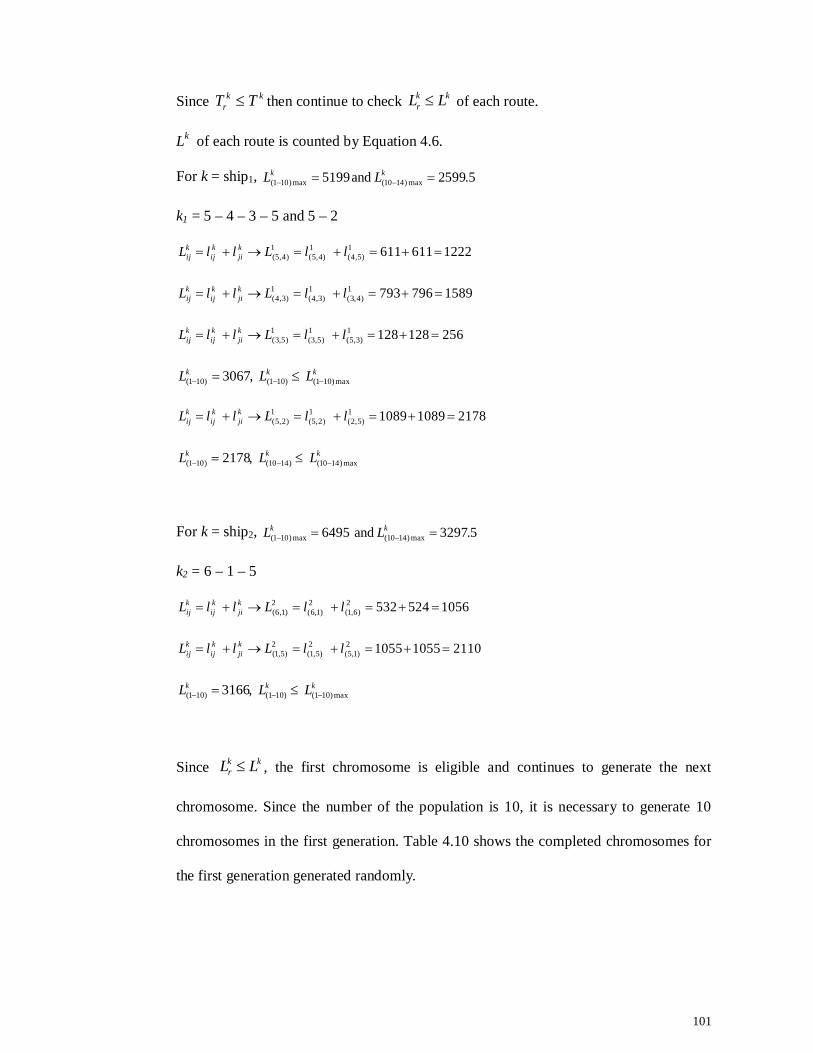
101

Since kkr TT then continue to check kk

r LL of each route.

Lk of each route is counted by Equation 4.6.

For k = ship1, 5.5992 and 5199 max)1410(max)101( kk LL

k1 = 5 – 4 – 3 – 5 and 5 – 2

12226116111)5,4(

1)4,5(

1)4,5( llLllL k

jikij

kij

15897967931)4,3(

1)3,4(

1)3,4( llLllL k

jikij

kij

2561281281)3,5(

1)5,3(

1)5,3( llLllL k

jikij

kij

kkk LLL max)101()101()101( ,3067

2178108910891)5,2(

1)2,5(

1)2,5( llLllL k

jikij

kij

kkk LLL max)1410()1410()101( ,2178

For k = ship2, 5.3297 and 6495 max)1410(max)101( kk LL

k2 = 6 – 1 – 5

10565245322)6,1(

2)1,6(

2)1,6( llLllL k

jikij

kij

2110105510552)1,5(

2)5,1(

2)5,1( llLllL k

jikij

kij

kkk LLL max)101()101()101( ,3166

Since kkr LL , the first chromosome is eligible and continues to generate the next

chromosome. Since the number of the population is 10, it is necessary to generate 10

chromosomes in the first generation. Table 4.10 shows the completed chromosomes for

the first generation generated randomly.

102

Phase 3: Evaluate the Fitness Value

In phase 3, the fitness value of the chromosome is calculated using Equation 4.11. The

fitness value is:

0.3948 1000000* 1

1

kkkkr ffff

f

Table 4.11 shows the completed fitness value of each chromosome.

103

Table 4.10 Chromosomes for the first generation

104

Table 4.11 Fitness value of each chromosome

105

Phase 4: Roulette Wheel Selection

This phase shows the process of roulette wheel selection. It is constructed as follows:

Step 1: Calculate the fitness value eval(vk) for each chromosome vk.

)()(e xfvval k k =1, 2, ..., pop_size

The fitness values for each chromosome are in Table 4.11.

Step 2: Calculate the total fitness of the population:

)( pop_size

1kkvevalF

9.3948 10

1k

)eval(vF k

Step 3: Calculate the selection probability )( sp of each chromosome s.

Total fitness F of the population is 9.3948, so the selection probabilities kp of

each chromosome are:

For the first chromosome, s = 1.

0.0982 9.3948 0.9226 ,)( 1 p

Fvevalp k

k

The second chromosome, s = 2

0.1033 9.3948 0.9709 ,)( 2 p

Fvevalp k

k

The complete value of kp is in the Table 4.12.

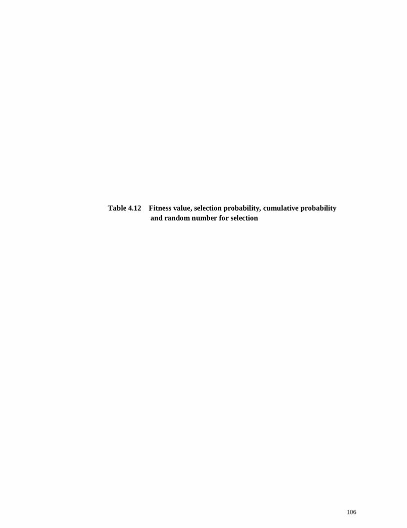
106

Table 4.12 Fitness value, selection probability, cumulative probability and random number for selection

107

Step 4: Calculate the cumulative probability kq of each chromosome s.

The cumulative probabilities kq for each chromosome are calculated as:

0.098211 pq

0.20150.10330.0982212 pqq

0.30690.10540.2015323 pqq

The complete value of )( kq that can be seen in the Table 4.12.

The selection process begins by spinning the roulette wheel n times, n the being

population size; each time a single chromosome is selected for the new population. If the

population size is 10, it is necessary to sequence 10 random numbers in a range [0, 1].

Let us assume that there is a random sequence of 10 numbers as shown in Table 4.12.

The first random number is r1 = 0.6957; 8171 qrandqr , meaning that chromosome

s8 is selected for the new population. The second random number is r2 = 0.7244;

8272 qrandqr , meaning that chromosome s8 is also selected for the new

population. The third random number is r3 = 0.4407; 5343 qrandqr , meaning that

chromosome s5 is again selected for the new population, and so on. After reviewing all

the numbers, the new population consists of the chromosomes as shown in Table 4.13.

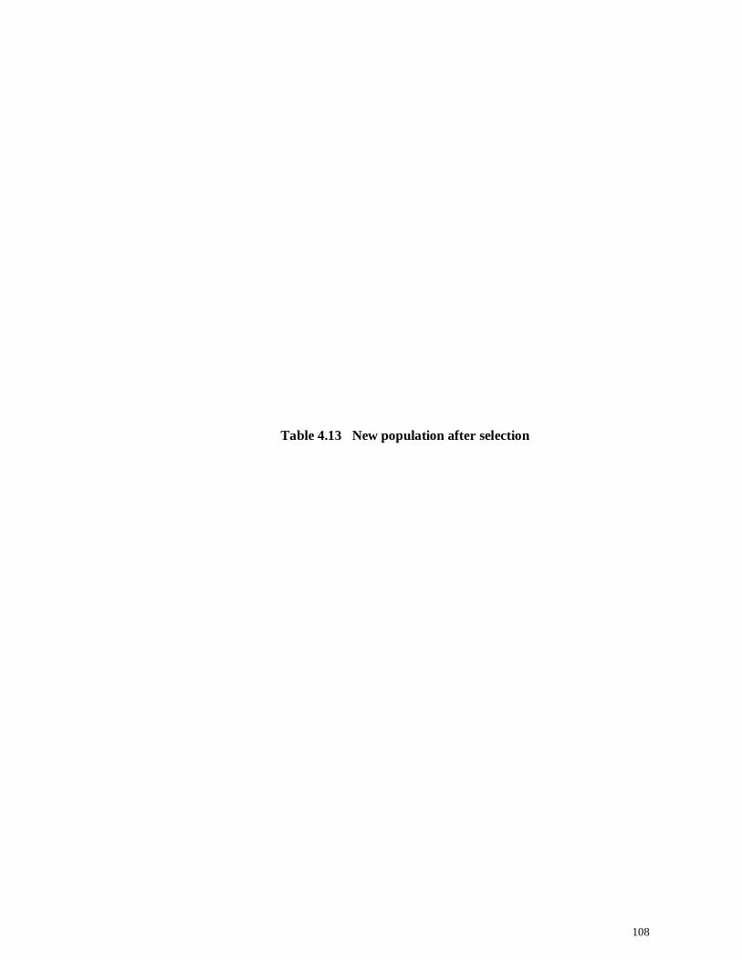
108

Table 4.13 New population after selection

109

Table 4.14 Check eligibility for crossover

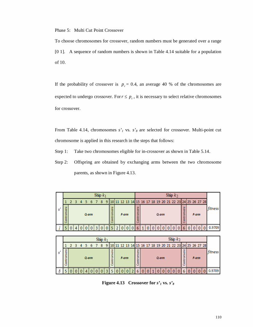
110

Phase 5: Multi Cut Point Crossover

To choose chromosomes for crossover, random numbers must be generated over a range

[0 1]. A sequence of random numbers is shown in Table 4.14 suitable for a population

of 10.

If the probability of crossover is cp = 0.4, an average 40 % of the chromosomes are

expected to undergo crossover. For cpr , it is necessary to select relative chromosomes

for crossover.

From Table 4.14, chromosomes s’1 vs. s’8 are selected for crossover. Multi-point cut

chromosome is applied in this research in the steps that follows:

Step 1: Take two chromosomes eligible for in-crossover as shown in Table 5.14.

Step 2: Offspring are obtained by exchanging arms between the two chromosome

parents, as shown in Figure 4.13.

Figure 4.13 Crossover for s’1 vs. s’8

111

Step 3: Check if arms exchanged qualify as feasible chromosomes. Check whether P-

arm exchanged qualifies as a feasible chromosome. If the offspring has

violated a constraint it needs to be repaired.

Complete results of the new chromosome structure after crossover are shown in Table

4.15.

112

Table 4.15 New population after crossover

113

Table 4.16 Fitness value and random number for mutation

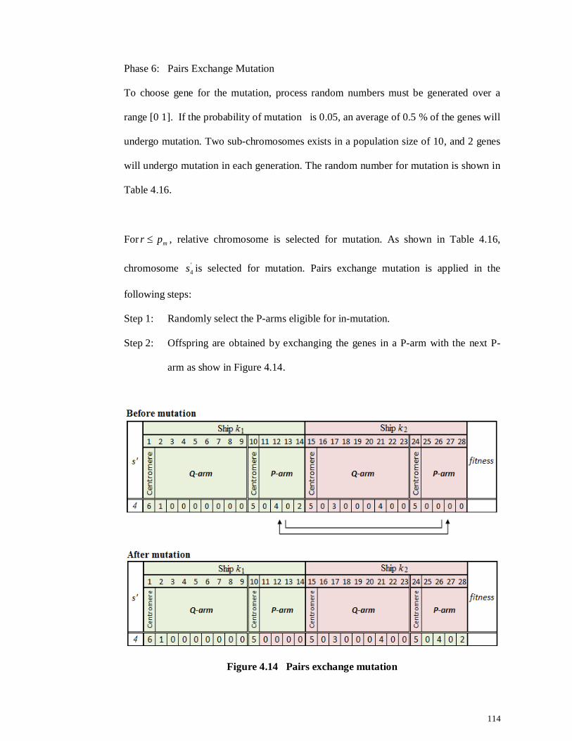
114

Phase 6: Pairs Exchange Mutation

To choose gene for the mutation, process random numbers must be generated over a

range [0 1]. If the probability of mutation is 0.05, an average of 0.5 % of the genes will

undergo mutation. Two sub-chromosomes exists in a population size of 10, and 2 genes

will undergo mutation in each generation. The random number for mutation is shown in

Table 4.16.

For mpr , relative chromosome is selected for mutation. As shown in Table 4.16,

chromosome '4s is selected for mutation. Pairs exchange mutation is applied in the

following steps:

Step 1: Randomly select the P-arms eligible for in-mutation.

Step 2: Offspring are obtained by exchanging the genes in a P-arm with the next P-

arm as show in Figure 4.14.

Figure 4.14 Pairs exchange mutation

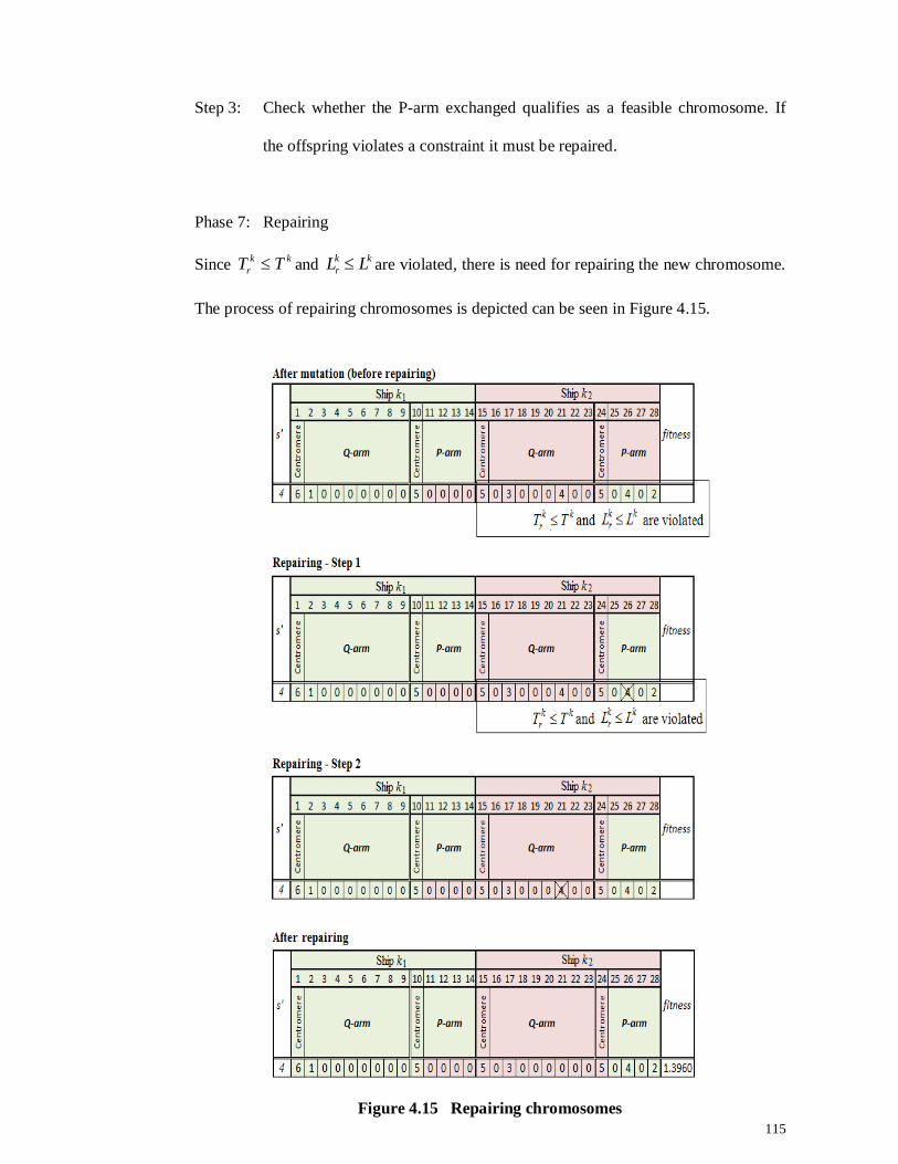
115

Step 3: Check whether the P-arm exchanged qualifies as a feasible chromosome. If

the offspring violates a constraint it must be repaired.

Phase 7: Repairing

Since kkr TT and kk

r LL are violated, there is need for repairing the new chromosome.

The process of repairing chromosomes is depicted can be seen in Figure 4.15.

Figure 4.15 Repairing chromosomes

116

The process is as follows:

Step 1: If kkr TT and kk

r LL are violated, check similar numbers in the same arm in

the same sub-chromosome and remove them. Since kkr TT and kk

r LL are

still violated, go to step 2.

Step 2: If kkr TT and kk

r LL are violated, check similar numbers in different arms

within the same sub-chromosomes and remove them.

Complete results of the structure of the new chromosome after mutation are shown in the

Table 4.17. The new population after mutation is the one used in the next generation.

Next iteration of Genetic Algorithm is completed. The test run is terminated after 100

generations (maximum generation). The best chromosome out of the 100 generations is

as follows:

Ship k = 1 serves route r = 1 (ports: 6 – 1 – 5)

Fuel consumption = 548,592 litres

Average of load factor = 74%

Number of ports of call = 5

Ship k = 2 serves route r = 8 (ports: 5 – 3 – 5 – 4 – 2)

Fuel consumption = 163,723 litres

Average of load factor = 123%

Number of ports of call = 9

117

Table 4.17 New population

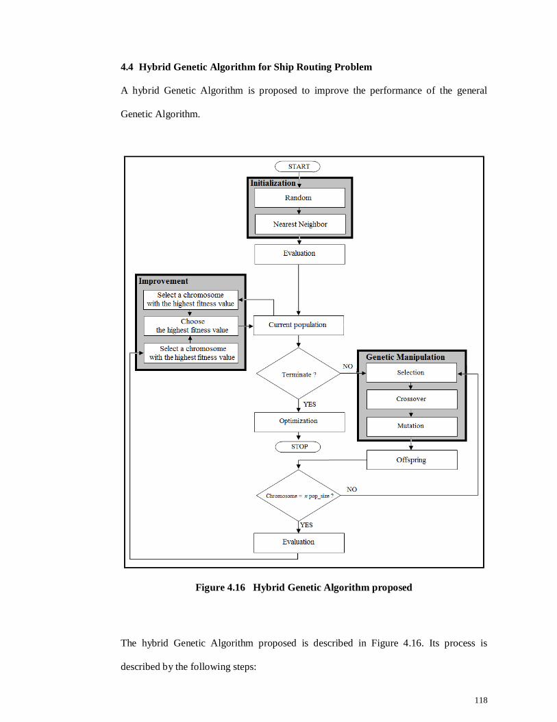
118

4.4 Hybrid Genetic Algorithm for Ship Routing Problem

A hybrid Genetic Algorithm is proposed to improve the performance of the general

Genetic Algorithm.

Figure 4.16 Hybrid Genetic Algorithm proposed

The hybrid Genetic Algorithm proposed is described in Figure 4.16. Its process is

described by the following steps:

119

Step 1: Represent a problem as a chromosome; choose a population size, the

crossover rate, and the mutation rate.

Step 2: Define a fitness function to measure the performance, or fitness, of an

individual chromosome in a problem domain.

Step 3: Generate chromosomes in a population of size, pop_size.

Centromeres generated randomly

Q-arm and P-arm generated by nearest neighbour method

Step 4: Calculate the fitness value of each chromosome. The chromosome with the

highest value saved into temporary memory.

Step 5: Select a chromosome from the current population.

Step 6: Create offspring by using crossover and mutation.

Step 7: Place the created offspring chromosomes in the new population.

Step 8: Repeat step 5 until the number of chromosomes is equal to the population

size.

Step 9: Replace the parents with the new population (offspring).

Step 10: Calculate of the fitness value of each chromosome. The chromosome with

the highest value is saved into temporary memory. Compare the two

chromosomes that are saved in temporary memory. The chromosome with

the highest fitness value replaces the other and is chosen for the next

population.

Step 11: Go to Step 4, and repeat the process until the termination criteria are

satisfied.

A chromosome in the hybrid Genetic Algorithm employed is represented similarly to in

a general Genetic Algorithm. The fitness function is also similar, but it differs in how

chromosomes are generated in the initial population. The initial population’s

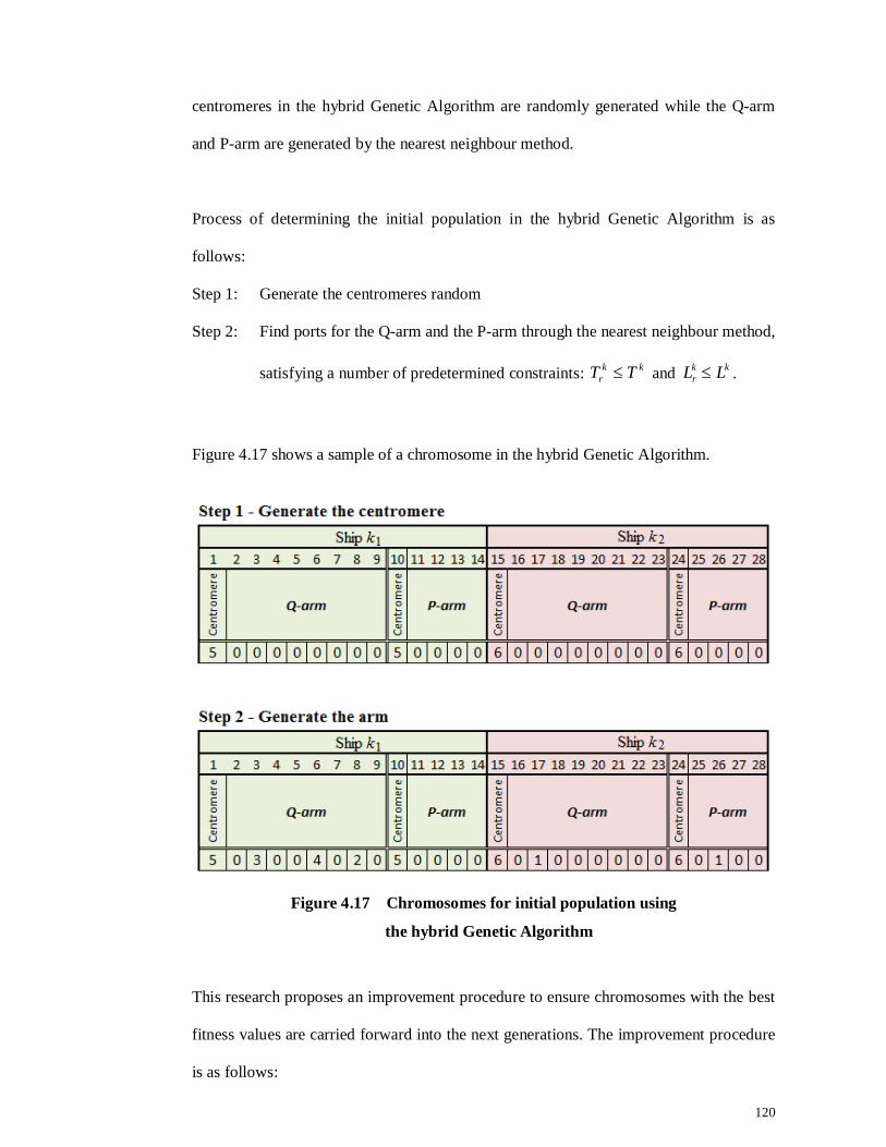
120

centromeres in the hybrid Genetic Algorithm are randomly generated while the Q-arm

and P-arm are generated by the nearest neighbour method.

Process of determining the initial population in the hybrid Genetic Algorithm is as

follows:

Step 1: Generate the centromeres random

Step 2: Find ports for the Q-arm and the P-arm through the nearest neighbour method,

satisfying a number of predetermined constraints: kkr TT and kk

r LL .

Figure 4.17 shows a sample of a chromosome in the hybrid Genetic Algorithm.

Figure 4.17 Chromosomes for initial population using

the hybrid Genetic Algorithm

This research proposes an improvement procedure to ensure chromosomes with the best

fitness values are carried forward into the next generations. The improvement procedure

is as follows:

121

Step 1: Calculate the fitness value of the parent’s chromosomes with the highest

fitness values are saved into temporary memory.

Step 2: Selection and recombination process is carried out for the offspring.

Step 3: Calculate fitness values of the offspring, and chromosomes with the highest

fitness values are saved into temporary memory.

Step 4: Compare the chromosomes saved in temporary memory. Chromosome with

the highest fitness values replace the others and are chosen for the next

population.

4.5 Summary

Three methods were used to solve a ship routing problem in the case study i.e. a

heuristic algorithm, a general Genetic Algorithm and a hybrid Genetic Algorithm.

The heuristic procedure involved three algorithm phases, namely clustering, assigned

vehicle and finding the best routes by a combination of feasible solution.

Phase I aims to cluster routes and solve the problem based on the constraint of

travel time and distance allowed for each ship.

Phase II checks involves checking vehicles assigned in a cluster to ensure each

route has at least one fuel port. In this phase, fuel consumption is calculated.

Phase III involves developing a robust algorithm based on the maximum insertion

concept. The idea is to successively insert a route into the best combination of

routes with minimum fuel consumption.

In the hybrid Genetic Algorithm, the length of a chromosome depends on the number of

ships. Each ship is represented as a sub-chromosome and each sub-chromosome consists

of 14 genes. A sub-chromosome consists of a Q-arm, a P-arm and two centromeres. The

122

1st and the 10th genes are called centromeres, which contain values that refer to the fuel

port. The 2nd to the 9th genes are called the Q-arm, while the 11th to the 14th genes are

called the P-arm. The Q-arm and P-arm contain values that refer to the customer port.

Roulette wheel selection, multi cut point crossover, and pairs exchange mutation is

applied in the general Genetic Algorithm and the hybrid Genetic Algorithm. Using the

general Genetic Algorithm, the initial population is generated randomly. The initial

population in the hybrid Genetic Algorithm process is generated by a random mix using

the nearest neighbour method. An improvement procedure is proposed in the hybrid

Genetic Algorithm to ensure chromosomes with the best fitness are carried forward into

the next generation.

123

CHAPTER 5 RESULT AND ANALYSIS

In this chapter, the computational results of the heuristic algorithm, the general Genetic

Algorithm and the hybrid Genetic Algorithm methods proposed in Chapter 4 are

presented. All the computational experiments were carried out using an Intel(R)

Core(TM) i5 CPU M430 @2.27GHz.

5.1 Experiment 1 - Performance of Three Algorithms Compared with Prior Work

The first experiment described herein examined the performance of the three algorithms

i.e. the heuristic algorithm, general genetic algorithm and proposed hybrid genetic

algorithm. It was compared with the existing route. Since there was no information

about the method used to generate the existing route, for simplicity the PELNI method

(PELNI, 2010) was denoted for use.

5.1.1 The Benchmarks Problem

Since there was no vehicle routing problem that was exactly similar to the problem

needing to be solved in the case study, the benchmarks were generated based on the

existing routes in the PT. PELNI for 2010. The benchmarks were generated to represent

different performances, i.e.:

40c-9d-8k = routes served by ships where capacity is 1000 - 1500 seats

28c-9d-9k = routes where the number of ports of call is 10 - 15

45c-11d-11k = routes where the number of ports of call is 16 - 20

32c-4d-8k = routes where the number of ports of call is 20 and above

34c-11d-11k = routes where the number of ports of call is 16 and less

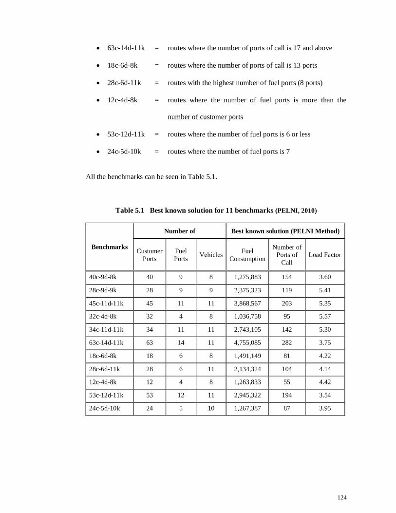
124

63c-14d-11k = routes where the number of ports of call is 17 and above

18c-6d-8k = routes where the number of ports of call is 13 ports

28c-6d-11k = routes with the highest number of fuel ports (8 ports)

12c-4d-8k = routes where the number of fuel ports is more than the

number of customer ports

53c-12d-11k = routes where the number of fuel ports is 6 or less

24c-5d-10k = routes where the number of fuel ports is 7

All the benchmarks can be seen in Table 5.1.

Table 5.1 Best known solution for 11 benchmarks (PELNI, 2010)

Benchmarks

Number of Best known solution (PELNI Method)

Customer Ports

Fuel Ports Vehicles Fuel

Consumption

Number of Ports of

Call Load Factor

40c-9d-8k 40 9 8 1,275,883 154 3.60

28c-9d-9k 28 9 9 2,375,323 119 5.41

45c-11d-11k 45 11 11 3,868,567 203 5.35

32c-4d-8k 32 4 8 1,036,758 95 5.57

34c-11d-11k 34 11 11 2,743,105 142 5.30

63c-14d-11k 63 14 11 4,755,085 282 3.75

18c-6d-8k 18 6 8 1,491,149 81 4.22

28c-6d-11k 28 6 11 2,134,324 104 4.14

12c-4d-8k 12 4 8 1,263,833 55 4.42

53c-12d-11k 53 12 11 2,945,322 194 3.54

24c-5d-10k 24 5 10 1,267,387 87 3.95

125

Figure 5.1 Routes of the benchmark; 40c-9d-8k

126

Figure 5.2 Routes of the benchmark; 28c-9d-9k

127

Figure 5.3 Routes of the benchmark; 45c-11d-11k

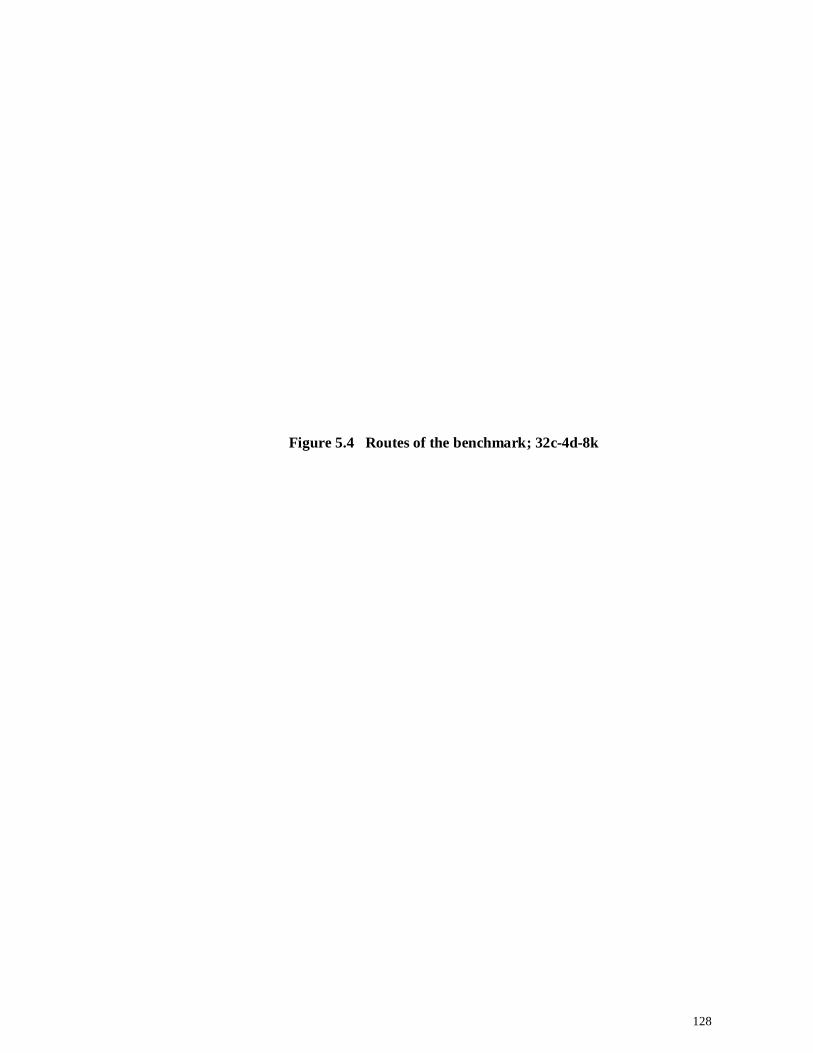
128

Figure 5.4 Routes of the benchmark; 32c-4d-8k

129

Figure 5.5 Routes of the benchmark; 34c-11d-11k

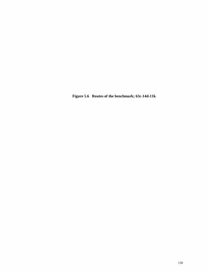
130

Figure 5.6 Routes of the benchmark; 63c-14d-11k

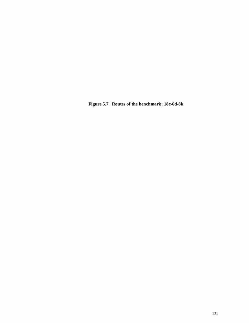
131

Figure 5.7 Routes of the benchmark; 18c-6d-8k

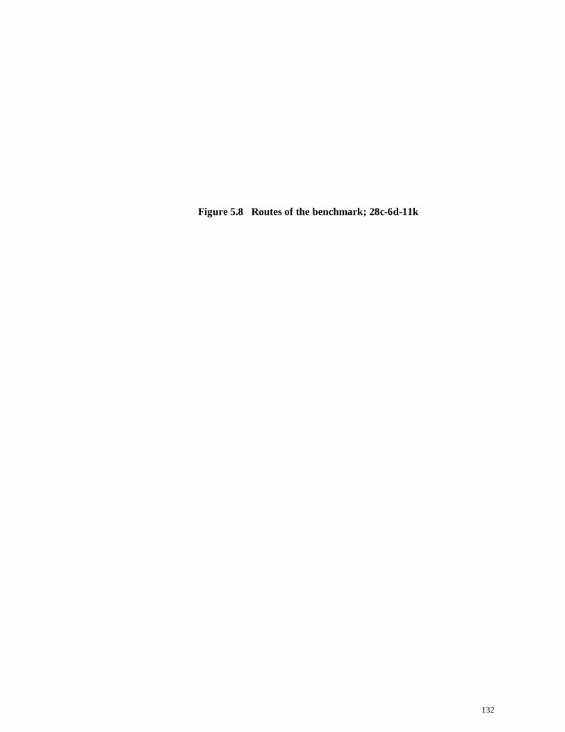
132

Figure 5.8 Routes of the benchmark; 28c-6d-11k

133

Figure 5.9 Routes of the benchmark; 12c-4d-8k

134

Figure 5.10 Routes of the benchmark; 53c-12d-11k

135

Figure 5.11 Routes of the benchmark; 24c-5d-10k

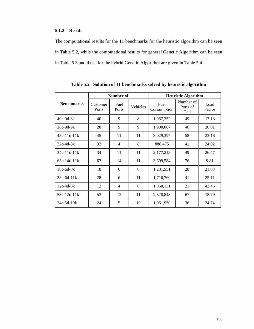
136

5.1.2 Result

The computational results for the 11 benchmarks for the heuristic algorithm can be seen

in Table 5.2, while the computational results for general Genetic Algorithm can be seen

in Table 5.3 and those for the hybrid Genetic Algorithm are given in Table 5.4.

Table 5.2 Solution of 11 benchmarks solved by heuristic algorithm

Benchmarks

Number of Heuristic Algorithm

Customer Ports

Fuel Ports Vehicles Fuel

Consumption

Number of Ports of

Call

Load Factor

40c-9d-8k 40 9 8 1,067,352 49 17.13

28c-9d-9k 28 9 9 1,900,067 40 26.01

45c-11d-11k 45 11 11 3,029,397 58 23.16

32c-4d-8k 32 4 8 888,475 41 24.02

34c-11d-11k 34 11 11 2,177,213 49 26.47

63c-14d-11k 63 14 11 3,699,584 76 9.81

18c-6d-8k 18 6 8 1,231,551 28 21.03

28c-6d-11k 28 6 11 1,716,760 41 25.11

12c-4d-8k 12 4 8 1,060,131 21 42.45

53c-12d-11k 53 12 11 2,328,848 67 18.79

24c-5d-10k 24 5 10 1,061,950 36 24.74

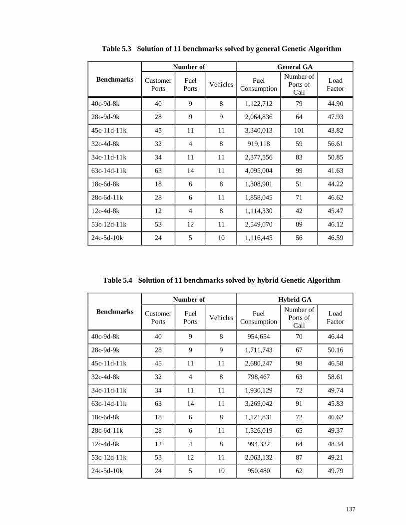
137

Table 5.3 Solution of 11 benchmarks solved by general Genetic Algorithm

Benchmarks

Number of General GA

Customer Ports

Fuel Ports Vehicles Fuel

Consumption

Number of Ports of

Call

Load Factor

40c-9d-8k 40 9 8 1,122,712 79 44.90

28c-9d-9k 28 9 9 2,064,836 64 47.93

45c-11d-11k 45 11 11 3,340,013 101 43.82

32c-4d-8k 32 4 8 919,118 59 56.61

34c-11d-11k 34 11 11 2,377,556 83 50.85

63c-14d-11k 63 14 11 4,095,004 99 41.63

18c-6d-8k 18 6 8 1,308,901 51 44.22

28c-6d-11k 28 6 11 1,858,045 71 46.62

12c-4d-8k 12 4 8 1,114,330 42 45.47

53c-12d-11k 53 12 11 2,549,070 89 46.12

24c-5d-10k 24 5 10 1,116,445 56 46.59

Table 5.4 Solution of 11 benchmarks solved by hybrid Genetic Algorithm

Benchmarks

Number of Hybrid GA

Customer Ports

Fuel Ports Vehicles Fuel

Consumption

Number of Ports of

Call

Load Factor

40c-9d-8k 40 9 8 954,654 70 46.44

28c-9d-9k 28 9 9 1,711,743 67 50.16

45c-11d-11k 45 11 11 2,680,247 98 46.58

32c-4d-8k 32 4 8 798,467 63 58.61

34c-11d-11k 34 11 11 1,930,129 72 49.74

63c-14d-11k 63 14 11 3,269,042 91 45.83

18c-6d-8k 18 6 8 1,121,831 72 46.62

28c-6d-11k 28 6 11 1,526,019 65 49.37

12c-4d-8k 12 4 8 994,332 64 48.34

53c-12d-11k 53 12 11 2,063,132 87 49.21

24c-5d-10k 24 5 10 950,480 62 49.79

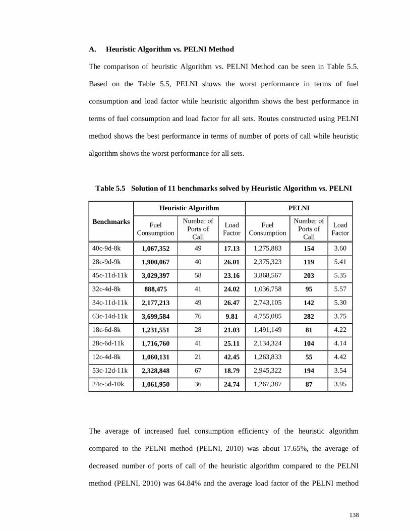
138

A. Heuristic Algorithm vs. PELNI Method

The comparison of heuristic Algorithm vs. PELNI Method can be seen in Table 5.5.

Based on the Table 5.5, PELNI shows the worst performance in terms of fuel

consumption and load factor while heuristic algorithm shows the best performance in

terms of fuel consumption and load factor for all sets. Routes constructed using PELNI

method shows the best performance in terms of number of ports of call while heuristic

algorithm shows the worst performance for all sets.

Table 5.5 Solution of 11 benchmarks solved by Heuristic Algorithm vs. PELNI

Benchmarks

Heuristic Algorithm PELNI

Fuel Consumption

Number of Ports of

Call

Load Factor

Fuel Consumption

Number of Ports of

Call

Load Factor

40c-9d-8k 1,067,352 49 17.13 1,275,883 154 3.60

28c-9d-9k 1,900,067 40 26.01 2,375,323 119 5.41

45c-11d-11k 3,029,397 58 23.16 3,868,567 203 5.35

32c-4d-8k 888,475 41 24.02 1,036,758 95 5.57

34c-11d-11k 2,177,213 49 26.47 2,743,105 142 5.30

63c-14d-11k 3,699,584 76 9.81 4,755,085 282 3.75

18c-6d-8k 1,231,551 28 21.03 1,491,149 81 4.22

28c-6d-11k 1,716,760 41 25.11 2,134,324 104 4.14

12c-4d-8k 1,060,131 21 42.45 1,263,833 55 4.42

53c-12d-11k 2,328,848 67 18.79 2,945,322 194 3.54

24c-5d-10k 1,061,950 36 24.74 1,267,387 87 3.95

The average of increased fuel consumption efficiency of the heuristic algorithm

compared to the PELNI method (PELNI, 2010) was about 17.65%, the average of

decreased number of ports of call of the heuristic algorithm compared to the PELNI

method (PELNI, 2010) was 64.84% and the average load factor of the PELNI method

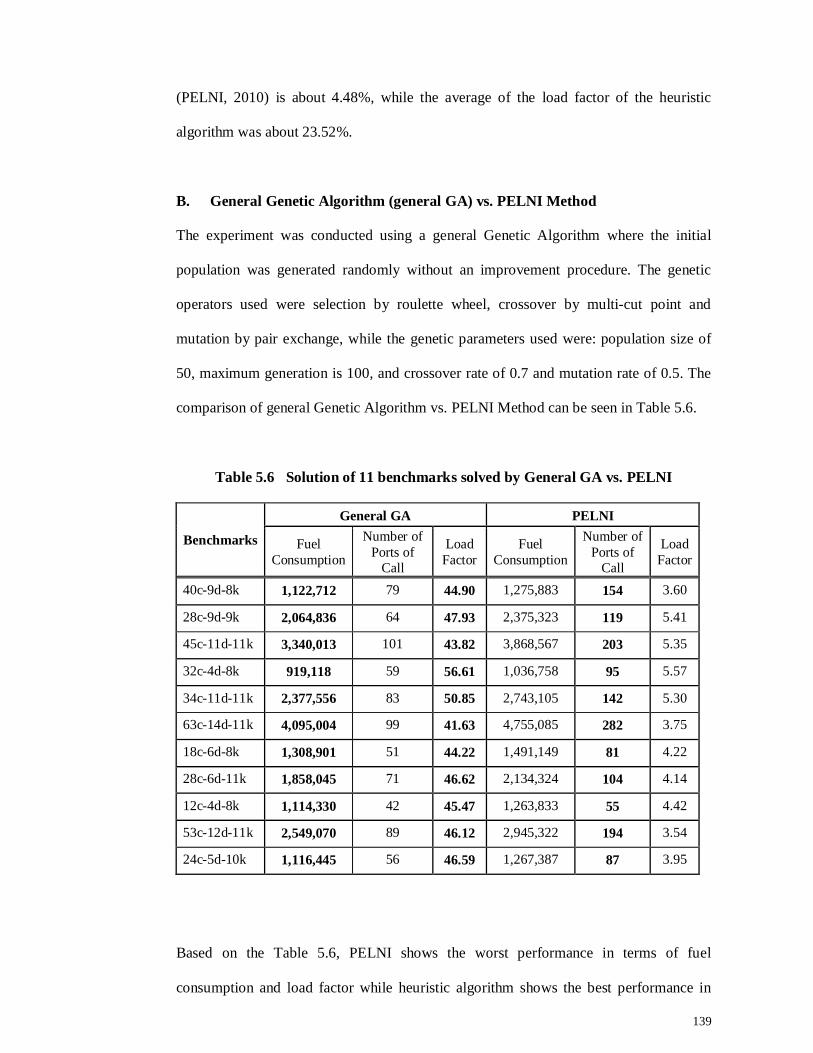
139

(PELNI, 2010) is about 4.48%, while the average of the load factor of the heuristic

algorithm was about 23.52%.

B. General Genetic Algorithm (general GA) vs. PELNI Method

The experiment was conducted using a general Genetic Algorithm where the initial

population was generated randomly without an improvement procedure. The genetic

operators used were selection by roulette wheel, crossover by multi-cut point and

mutation by pair exchange, while the genetic parameters used were: population size of

50, maximum generation is 100, and crossover rate of 0.7 and mutation rate of 0.5. The

comparison of general Genetic Algorithm vs. PELNI Method can be seen in Table 5.6.

Table 5.6 Solution of 11 benchmarks solved by General GA vs. PELNI

Benchmarks

General GA PELNI

Fuel Consumption

Number of Ports of

Call

Load Factor

Fuel Consumption

Number of Ports of

Call

Load Factor

40c-9d-8k 1,122,712 79 44.90 1,275,883 154 3.60

28c-9d-9k 2,064,836 64 47.93 2,375,323 119 5.41

45c-11d-11k 3,340,013 101 43.82 3,868,567 203 5.35

32c-4d-8k 919,118 59 56.61 1,036,758 95 5.57

34c-11d-11k 2,377,556 83 50.85 2,743,105 142 5.30

63c-14d-11k 4,095,004 99 41.63 4,755,085 282 3.75

18c-6d-8k 1,308,901 51 44.22 1,491,149 81 4.22

28c-6d-11k 1,858,045 71 46.62 2,134,324 104 4.14

12c-4d-8k 1,114,330 42 45.47 1,263,833 55 4.42

53c-12d-11k 2,549,070 89 46.12 2,945,322 194 3.54

24c-5d-10k 1,116,445 56 46.59 1,267,387 87 3.95

Based on the Table 5.6, PELNI shows the worst performance in terms of fuel

consumption and load factor while heuristic algorithm shows the best performance in

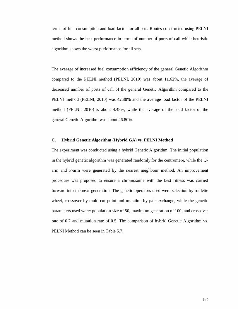
140

terms of fuel consumption and load factor for all sets. Routes constructed using PELNI

method shows the best performance in terms of number of ports of call while heuristic

algorithm shows the worst performance for all sets.

The average of increased fuel consumption efficiency of the general Genetic Algorithm

compared to the PELNI method (PELNI, 2010) was about 11.62%, the average of

decreased number of ports of call of the general Genetic Algorithm compared to the

PELNI method (PELNI, 2010) was 42.88% and the average load factor of the PELNI

method (PELNI, 2010) is about 4.48%, while the average of the load factor of the

general Genetic Algorithm was about 46.80%.

C. Hybrid Genetic Algorithm (Hybrid GA) vs. PELNI Method

The experiment was conducted using a hybrid Genetic Algorithm. The initial population

in the hybrid genetic algorithm was generated randomly for the centromere, while the Q-

arm and P-arm were generated by the nearest neighbour method. An improvement

procedure was proposed to ensure a chromosome with the best fitness was carried

forward into the next generation. The genetic operators used were selection by roulette

wheel, crossover by multi-cut point and mutation by pair exchange, while the genetic

parameters used were: population size of 50, maximum generation of 100, and crossover

rate of 0.7 and mutation rate of 0.5. The comparison of hybrid Genetic Algorithm vs.

PELNI Method can be seen in Table 5.7.

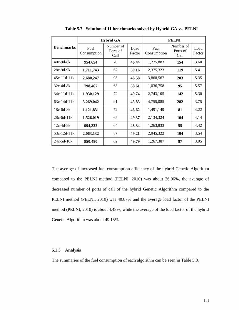
141

Table 5.7 Solution of 11 benchmarks solved by Hybrid GA vs. PELNI

Benchmarks

Hybrid GA PELNI

Fuel Consumption

Number of Ports of

Call

Load Factor

Fuel Consumption

Number of Ports of

Call

Load Factor

40c-9d-8k 954,654 70 46.44 1,275,883 154 3.60

28c-9d-9k 1,711,743 67 50.16 2,375,323 119 5.41

45c-11d-11k 2,680,247 98 46.58 3,868,567 203 5.35

32c-4d-8k 798,467 63 58.61 1,036,758 95 5.57

34c-11d-11k 1,930,129 72 49.74 2,743,105 142 5.30

63c-14d-11k 3,269,042 91 45.83 4,755,085 282 3.75

18c-6d-8k 1,121,831 72 46.62 1,491,149 81 4.22

28c-6d-11k 1,526,019 65 49.37 2,134,324 104 4.14

12c-4d-8k 994,332 64 48.34 1,263,833 55 4.42

53c-12d-11k 2,063,132 87 49.21 2,945,322 194 3.54

24c-5d-10k 950,480 62 49.79 1,267,387 87 3.95

The average of increased fuel consumption efficiency of the hybrid Genetic Algorithm

compared to the PELNI method (PELNI, 2010) was about 26.06%, the average of

decreased number of ports of call of the hybrid Genetic Algorithm compared to the

PELNI method (PELNI, 2010) was 40.87% and the average load factor of the PELNI

method (PELNI, 2010) is about 4.48%, while the average of the load factor of the hybrid

Genetic Algorithm was about 49.15%.

5.1.3 Analysis

The summaries of the fuel consumption of each algorithm can be seen in Table 5.8.

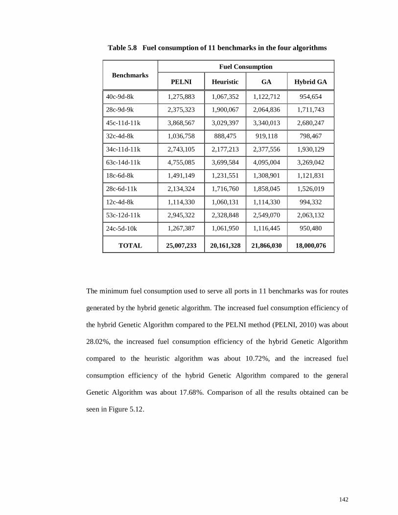
142

Table 5.8 Fuel consumption of 11 benchmarks in the four algorithms

Benchmarks Fuel Consumption

PELNI Heuristic GA Hybrid GA

40c-9d-8k 1,275,883 1,067,352 1,122,712 954,654

28c-9d-9k 2,375,323 1,900,067 2,064,836 1,711,743

45c-11d-11k 3,868,567 3,029,397 3,340,013 2,680,247

32c-4d-8k 1,036,758 888,475 919,118 798,467

34c-11d-11k 2,743,105 2,177,213 2,377,556 1,930,129

63c-14d-11k 4,755,085 3,699,584 4,095,004 3,269,042

18c-6d-8k 1,491,149 1,231,551 1,308,901 1,121,831

28c-6d-11k 2,134,324 1,716,760 1,858,045 1,526,019

12c-4d-8k 1,114,330 1,060,131 1,114,330 994,332

53c-12d-11k 2,945,322 2,328,848 2,549,070 2,063,132

24c-5d-10k 1,267,387 1,061,950 1,116,445 950,480

TOTAL 25,007,233 20,161,328 21,866,030 18,000,076

The minimum fuel consumption used to serve all ports in 11 benchmarks was for routes

generated by the hybrid genetic algorithm. The increased fuel consumption efficiency of

the hybrid Genetic Algorithm compared to the PELNI method (PELNI, 2010) was about

28.02%, the increased fuel consumption efficiency of the hybrid Genetic Algorithm

compared to the heuristic algorithm was about 10.72%, and the increased fuel

consumption efficiency of the hybrid Genetic Algorithm compared to the general

Genetic Algorithm was about 17.68%. Comparison of all the results obtained can be

seen in Figure 5.12.

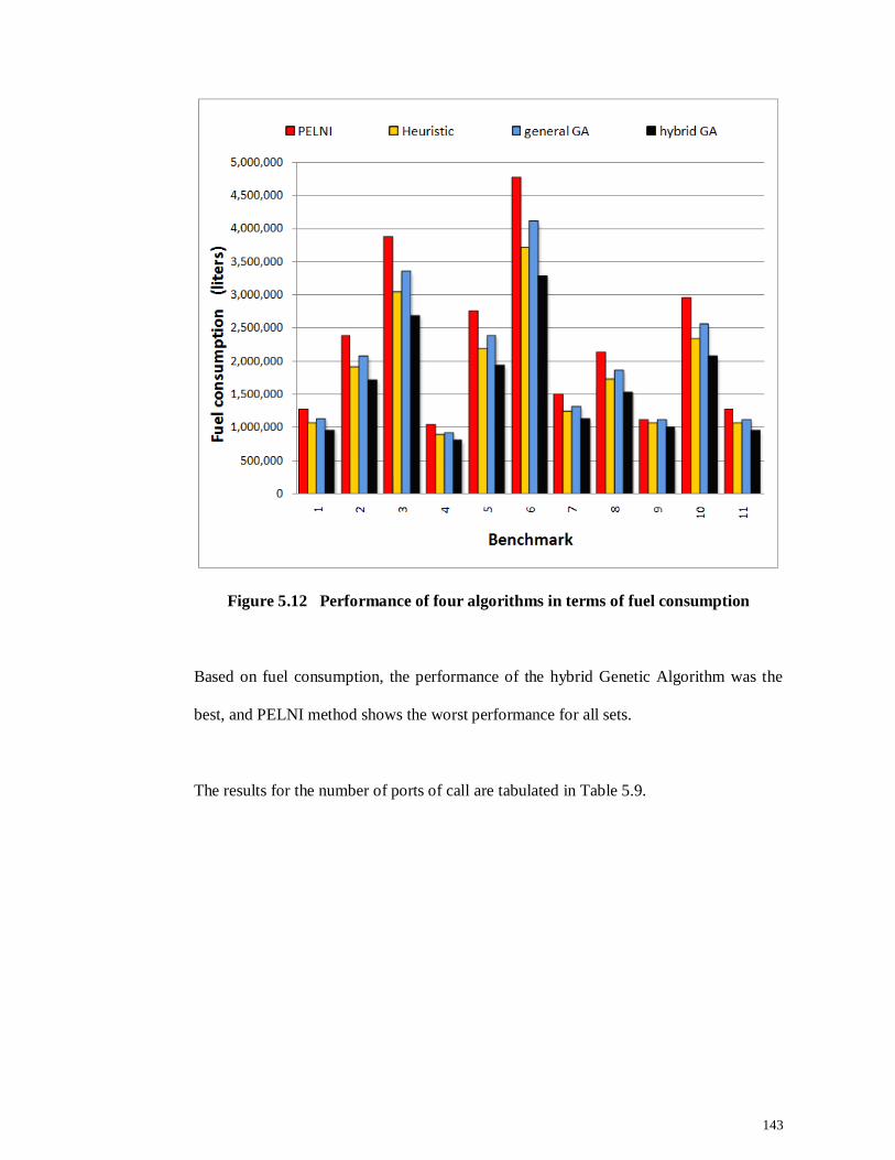
143

Figure 5.12 Performance of four algorithms in terms of fuel consumption

Based on fuel consumption, the performance of the hybrid Genetic Algorithm was the

best, and PELNI method shows the worst performance for all sets.

The results for the number of ports of call are tabulated in Table 5.9.

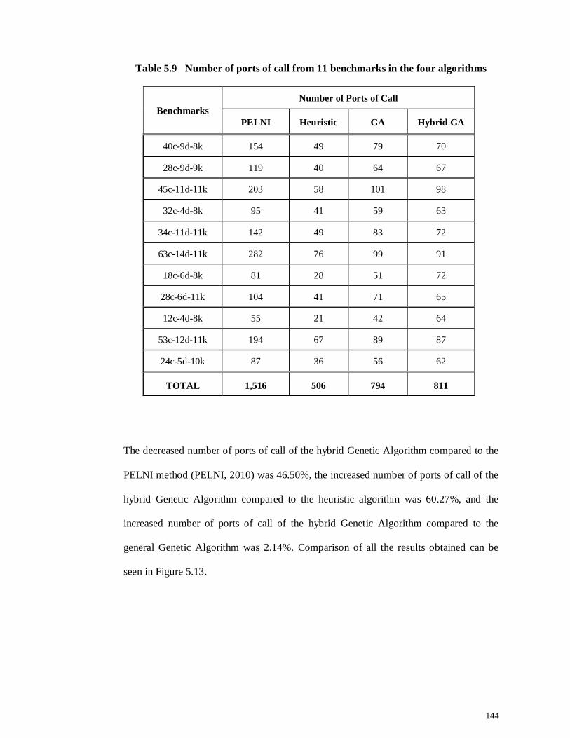
144

Table 5.9 Number of ports of call from 11 benchmarks in the four algorithms

Benchmarks Number of Ports of Call

PELNI Heuristic GA Hybrid GA

40c-9d-8k 154 49 79 70

28c-9d-9k 119 40 64 67

45c-11d-11k 203 58 101 98

32c-4d-8k 95 41 59 63

34c-11d-11k 142 49 83 72

63c-14d-11k 282 76 99 91

18c-6d-8k 81 28 51 72

28c-6d-11k 104 41 71 65

12c-4d-8k 55 21 42 64

53c-12d-11k 194 67 89 87

24c-5d-10k 87 36 56 62

TOTAL 1,516 506 794 811

The decreased number of ports of call of the hybrid Genetic Algorithm compared to the

PELNI method (PELNI, 2010) was 46.50%, the increased number of ports of call of the

hybrid Genetic Algorithm compared to the heuristic algorithm was 60.27%, and the

increased number of ports of call of the hybrid Genetic Algorithm compared to the

general Genetic Algorithm was 2.14%. Comparison of all the results obtained can be

seen in Figure 5.13.

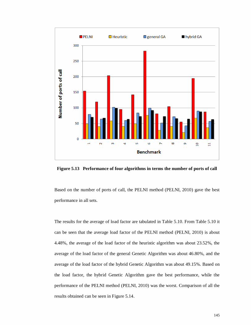
145

Figure 5.13 Performance of four algorithms in terms the number of ports of call

Based on the number of ports of call, the PELNI method (PELNI, 2010) gave the best

performance in all sets.

The results for the average of load factor are tabulated in Table 5.10. From Table 5.10 it

can be seen that the average load factor of the PELNI method (PELNI, 2010) is about

4.48%, the average of the load factor of the heuristic algorithm was about 23.52%, the

average of the load factor of the general Genetic Algorithm was about 46.80%, and the

average of the load factor of the hybrid Genetic Algorithm was about 49.15%. Based on

the load factor, the hybrid Genetic Algorithm gave the best performance, while the

performance of the PELNI method (PELNI, 2010) was the worst. Comparison of all the

results obtained can be seen in Figure 5.14.

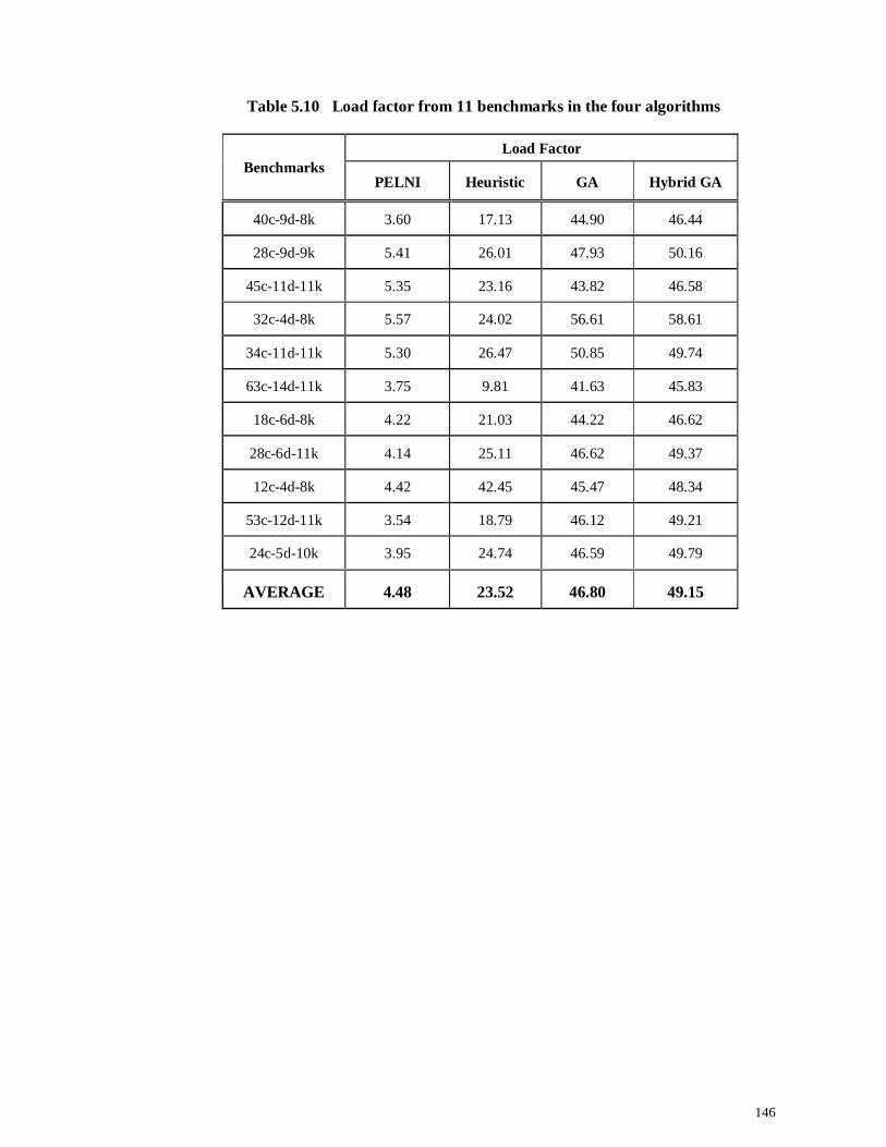
146

Table 5.10 Load factor from 11 benchmarks in the four algorithms

Benchmarks Load Factor

PELNI Heuristic GA Hybrid GA

40c-9d-8k 3.60 17.13 44.90 46.44

28c-9d-9k 5.41 26.01 47.93 50.16

45c-11d-11k 5.35 23.16 43.82 46.58

32c-4d-8k 5.57 24.02 56.61 58.61

34c-11d-11k 5.30 26.47 50.85 49.74

63c-14d-11k 3.75 9.81 41.63 45.83

18c-6d-8k 4.22 21.03 44.22 46.62

28c-6d-11k 4.14 25.11 46.62 49.37

12c-4d-8k 4.42 42.45 45.47 48.34

53c-12d-11k 3.54 18.79 46.12 49.21

24c-5d-10k 3.95 24.74 46.59 49.79

AVERAGE 4.48 23.52 46.80 49.15

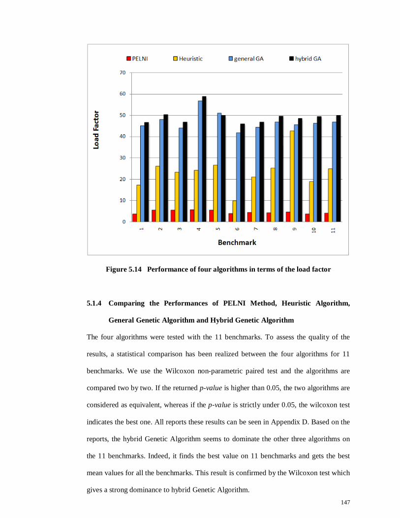
147

Figure 5.14 Performance of four algorithms in terms of the load factor

5.1.4 Comparing the Performances of PELNI Method, Heuristic Algorithm,

General Genetic Algorithm and Hybrid Genetic Algorithm

The four algorithms were tested with the 11 benchmarks. To assess the quality of the

results, a statistical comparison has been realized between the four algorithms for 11

benchmarks. We use the Wilcoxon non-parametric paired test and the algorithms are

compared two by two. If the returned p-value is higher than 0.05, the two algorithms are

considered as equivalent, whereas if the p-value is strictly under 0.05, the wilcoxon test

indicates the best one. All reports these results can be seen in Appendix D. Based on the

reports, the hybrid Genetic Algorithm seems to dominate the other three algorithms on

the 11 benchmarks. Indeed, it finds the best value on 11 benchmarks and gets the best

mean values for all the benchmarks. This result is confirmed by the Wilcoxon test which

gives a strong dominance to hybrid Genetic Algorithm.

148

5.2 Experiment 2 - Implementation of Algorithm

The second experiment was the implementation of algorithms for the ship routing of the

PT. PELNI. In 2010, the PT. PELNI operated a service of 25 passenger ships throughout

the Indonesian archipelago. The PT. PELNI served 84 ports and 12 of them were fuel

ports. Each ship served exactly one route and a route included by necessity at least one

fuel port.

5.2.1 Existing Routes in PT. PELNI 2010

Table 5.11 shows the fuel consumption, number of ports of call and load factor of routes

generated by the PELNI method (PELNI, 2010). Each route served by a ship where the

complete routes can be seen in Table 5.12.

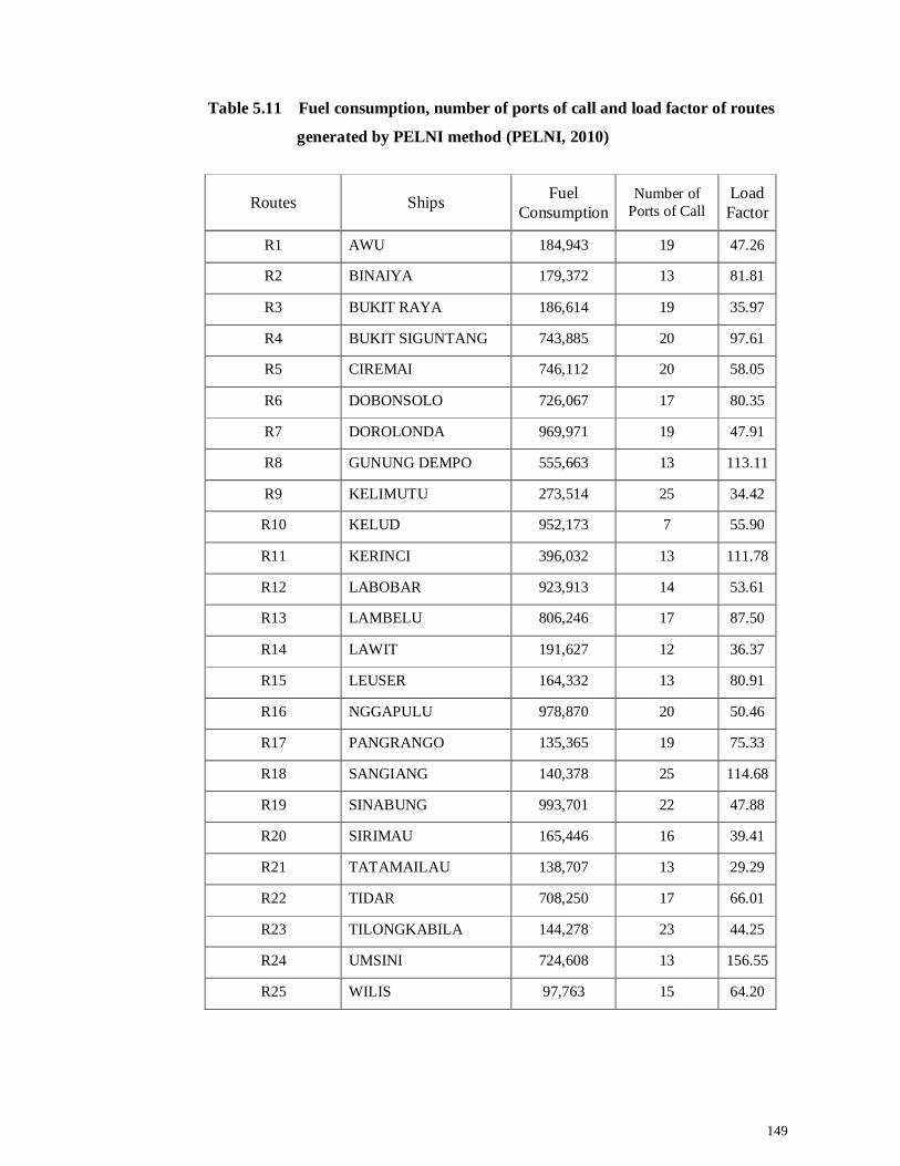
149

Table 5.11 Fuel consumption, number of ports of call and load factor of routes

generated by PELNI method (PELNI, 2010)

Routes Ships Fuel Consumption

Number of Ports of Call

Load Factor

R1 AWU 184,943 19 47.26

R2 BINAIYA 179,372 13 81.81

R3 BUKIT RAYA 186,614 19 35.97

R4 BUKIT SIGUNTANG 743,885 20 97.61

R5 CIREMAI 746,112 20 58.05

R6 DOBONSOLO 726,067 17 80.35

R7 DOROLONDA 969,971 19 47.91

R8 GUNUNG DEMPO 555,663 13 113.11

R9 KELIMUTU 273,514 25 34.42

R10 KELUD 952,173 7 55.90

R11 KERINCI 396,032 13 111.78

R12 LABOBAR 923,913 14 53.61

R13 LAMBELU 806,246 17 87.50

R14 LAWIT 191,627 12 36.37

R15 LEUSER 164,332 13 80.91

R16 NGGAPULU 978,870 20 50.46

R17 PANGRANGO 135,365 19 75.33

R18 SANGIANG 140,378 25 114.68

R19 SINABUNG 993,701 22 47.88

R20 SIRIMAU 165,446 16 39.41

R21 TATAMAILAU 138,707 13 29.29

R22 TIDAR 708,250 17 66.01

R23 TILONGKABILA 144,278 23 44.25

R24 UMSINI 724,608 13 156.55

R25 WILIS 97,763 15 64.20

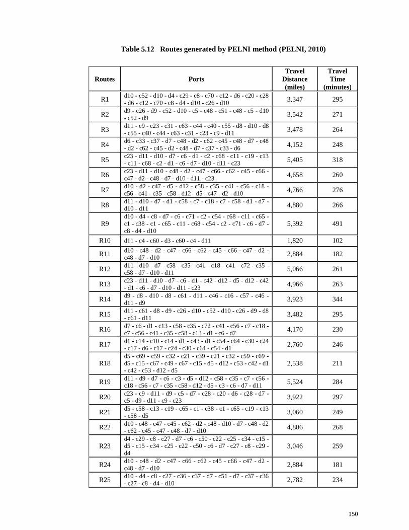
150

Table 5.12 Routes generated by PELNI method (PELNI, 2010)

Routes Ports Travel

Distance (miles)

Travel Time

(minutes)

R1 d10 - c52 - d10 - d4 - c29 - c8 - c70 - c12 - d6 - c20 - c28 - d6 - c12 - c70 - c8 - d4 - d10 - c26 - d10 3,347 295

R2 d9 - c26 - d9 - c52 - d10 - c5 - c48 - c51 - c48 - c5 - d10 - c52 - d9 3,542 271

R3 d11 - c9 - c23 - c31 - c63 - c44 - c40 - c55 - d8 - d10 - d8 - c55 - c40 - c44 - c63 - c31 - c23 - c9 - d11 3,478 264

R4 d6 - c33 - c37 - d7 - c48 - d2 - c62 - c45 - c48 - d7 - c48 - d2 - c62 - c45 - d2 - c48 - d7 - c37 - c33 - d6 4,152 248

R5 c23 - d11 - d10 - d7 - c6 - d1 - c2 - c68 - c11 - c19 - c13 - c11 - c68 - c2 - d1 - c6 - d7 - d10 - d11 - c23 5,405 318

R6 c23 - d11 - d10 - c48 - d2 - c47 - c66 - c62 - c45 - c66 - c47 - d2 - c48 - d7 - d10 - d11 - c23 4,658 260

R7 d10 - d2 - c47 - d5 - d12 - c58 - c35 - c41 - c56 - c18 - c56 - c41 - c35 - c58 - d12 - d5 - c47 - d2 - d10 4,766 276

R8 d11 - d10 - d7 - d1 - c58 - c7 - c18 - c7 - c58 - d1 - d7 - d10 - d11 4,880 266

R9 d10 - d4 - c8 - d7 - c6 - c71 - c2 - c54 - c68 - c11 - c65 - c1 - c38 - c1 - c65 - c11 - c68 - c54 - c2 - c71 - c6 - d7 - c8 - d4 - d10

5,392 491

R10 d11 - c4 - c60 - d3 - c60 - c4 - d11 1,820 102

R11 d10 - c48 - d2 - c47 - c66 - c62 - c45 - c66 - c47 - d2 - c48 - d7 - d10 2,884 182

R12 d11 - d10 - d7 - c58 - c35 - c41 - c18 - c41 - c72 - c35 - c58 - d7 - d10 - d11 5,066 261

R13 c23 - d11 - d10 - d7 - c6 - d1 - c42 - d12 - d5 - d12 - c42 - d1 - c6 - d7 - d10 - d11 - c23 4,966 263

R14 d9 - d8 - d10 - d8 - c61 - d11 - c46 - c16 - c57 - c46 - d11 - d9 3,923 344

R15 d11 - c61 - d8 - d9 - c26 - d10 - c52 - d10 - c26 - d9 - d8 - c61 - d11 3,482 295

R16 d7 - c6 - d1 - c13 - c58 - c35 - c72 - c41 - c56 - c7 - c18 - c7 - c56 - c41 - c35 - c58 - c13 - d1 - c6 - d7 4,170 230

R17 d1 - c14 - c10 - c14 - d1 - c43 - d1 - c54 - c64 - c30 - c24 - c17 - d6 - c17 - c24 - c30 - c64 - c54 - d1 2,760 246

R18 d5 - c69 - c59 - c32 - c21 - c39 - c21 - c32 - c59 - c69 - d5 - c15 - c67 - c49 - c67 - c15 - d5 - d12 - c53 - c42 - d1 - c42 - c53 - d12 - d5

2,538 211

R19 d11 - d9 - d7 - c6 - c3 - d5 - d12 - c58 - c35 - c7 - c56 - c18 - c56 - c7 - c35 - c58 - d12 - d5 - c3 - c6 - d7 - d11 5,524 284

R20 c23 - c9 - d11 - d9 - c5 - d7 - c28 - c20 - d6 - c28 - d7 - c5 - d9 - d11 - c9 - c23 3,922 297

R21 d5 - c58 - c13 - c19 - c65 - c1 - c38 - c1 - c65 - c19 - c13 - c58 - d5 3,060 249

R22 d10 - c48 - c47 - c45 - c62 - d2 - c48 - d10 - d7 - c48 - d2 - c62 - c45 - c47 - c48 - d7 - d10 4,806 268

R23 d4 - c29 - c8 - c27 - d7 - c6 - c50 - c22 - c25 - c34 - c15 - d5 - c15 - c34 - c25 - c22 - c50 - c6 - d7 - c27 - c8 - c29 - d4

3,046 259

R24 d10 - c48 - d2 - c47 - c66 - c62 - c45 - c66 - c47 - d2 - c48 - d7 - d10 2,884 181

R25 d10 - d4 - c8 - c27 - c36 - c37 - d7 - c51 - d7 - c37 - c36 - c27 - c8 - d4 - d10 2,782 234

151

Figure 5.15 Routes generated by PELNI method (PELNI, 2010)

152

5.2.2 Routes Generated Using a General Genetic Algorithm

The experiment in this part was to generate routes using a general Genetic Algorithm

that could be used in the real world. The first population was generated randomly

without an improvement procedure. The genetic operators used were selection by

roulette wheel, crossover by multi cut point and mutation by pair exchange, while the

genetic parameters used were: population size of 50, maximum generation of 100,

crossover rate of 0.7 and mutation rate of 0.5.

Fuel consumption, number of ports of call and load factor of routes generated by the

general Genetic Algorithm shown in Table 5.13. Each route served by a ship where the

complete routes can be seen in Table 5.14.

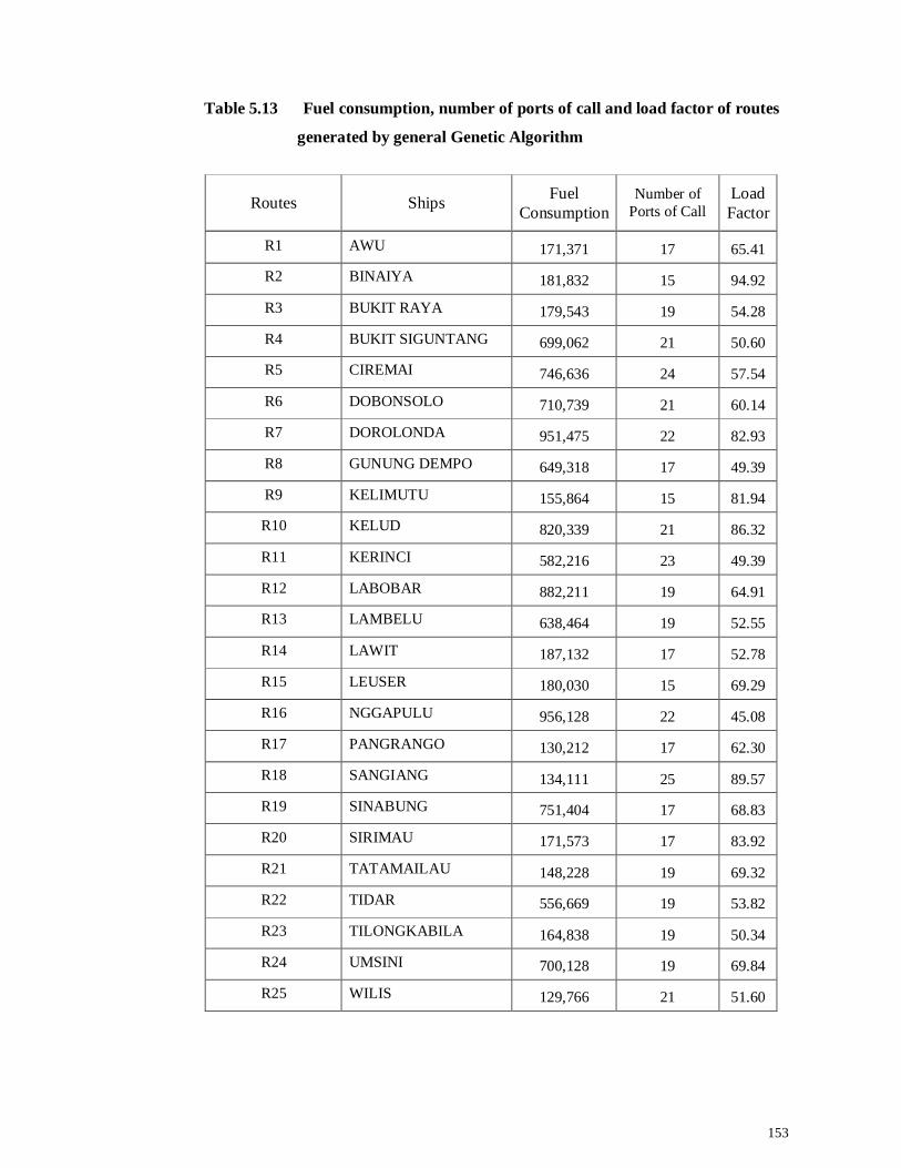
153

Table 5.13 Fuel consumption, number of ports of call and load factor of routes

generated by general Genetic Algorithm

Routes Ships Fuel Consumption

Number of Ports of Call

Load Factor

R1 AWU 171,371 17 65.41

R2 BINAIYA 181,832 15 94.92

R3 BUKIT RAYA 179,543 19 54.28

R4 BUKIT SIGUNTANG 699,062 21 50.60

R5 CIREMAI 746,636 24 57.54

R6 DOBONSOLO 710,739 21 60.14

R7 DOROLONDA 951,475 22 82.93

R8 GUNUNG DEMPO 649,318 17 49.39

R9 KELIMUTU 155,864 15 81.94

R10 KELUD 820,339 21 86.32

R11 KERINCI 582,216 23 49.39

R12 LABOBAR 882,211 19 64.91

R13 LAMBELU 638,464 19 52.55

R14 LAWIT 187,132 17 52.78

R15 LEUSER 180,030 15 69.29

R16 NGGAPULU 956,128 22 45.08

R17 PANGRANGO 130,212 17 62.30

R18 SANGIANG 134,111 25 89.57

R19 SINABUNG 751,404 17 68.83

R20 SIRIMAU 171,573 17 83.92

R21 TATAMAILAU 148,228 19 69.32

R22 TIDAR 556,669 19 53.82

R23 TILONGKABILA 164,838 19 50.34

R24 UMSINI 700,128 19 69.84

R25 WILIS 129,766 21 51.60

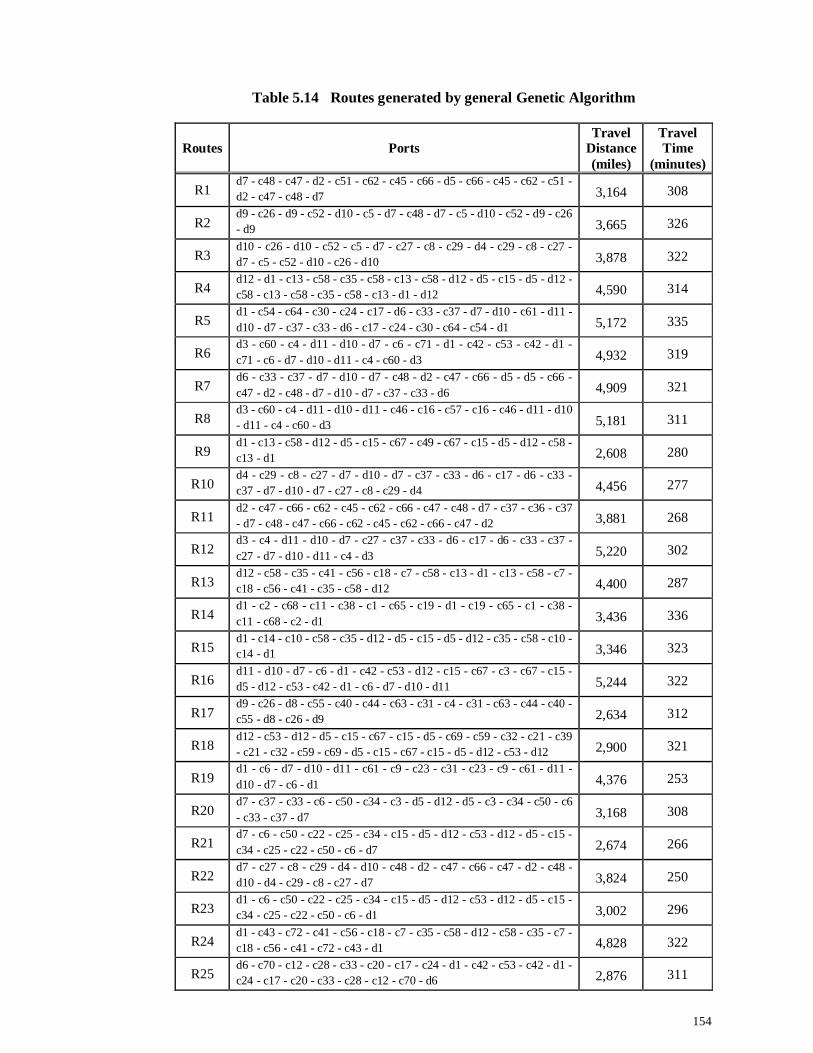
154

Table 5.14 Routes generated by general Genetic Algorithm

Routes Ports Travel

Distance (miles)

Travel Time

(minutes)

R1 d7 - c48 - c47 - d2 - c51 - c62 - c45 - c66 - d5 - c66 - c45 - c62 - c51 - d2 - c47 - c48 - d7 3,164 308

R2 d9 - c26 - d9 - c52 - d10 - c5 - d7 - c48 - d7 - c5 - d10 - c52 - d9 - c26 - d9 3,665 326

R3 d10 - c26 - d10 - c52 - c5 - d7 - c27 - c8 - c29 - d4 - c29 - c8 - c27 - d7 - c5 - c52 - d10 - c26 - d10 3,878 322

R4 d12 - d1 - c13 - c58 - c35 - c58 - c13 - c58 - d12 - d5 - c15 - d5 - d12 - c58 - c13 - c58 - c35 - c58 - c13 - d1 - d12 4,590 314

R5 d1 - c54 - c64 - c30 - c24 - c17 - d6 - c33 - c37 - d7 - d10 - c61 - d11 - d10 - d7 - c37 - c33 - d6 - c17 - c24 - c30 - c64 - c54 - d1 5,172 335

R6 d3 - c60 - c4 - d11 - d10 - d7 - c6 - c71 - d1 - c42 - c53 - c42 - d1 - c71 - c6 - d7 - d10 - d11 - c4 - c60 - d3 4,932 319

R7 d6 - c33 - c37 - d7 - d10 - d7 - c48 - d2 - c47 - c66 - d5 - d5 - c66 - c47 - d2 - c48 - d7 - d10 - d7 - c37 - c33 - d6 4,909 321

R8 d3 - c60 - c4 - d11 - d10 - d11 - c46 - c16 - c57 - c16 - c46 - d11 - d10 - d11 - c4 - c60 - d3 5,181 311

R9 d1 - c13 - c58 - d12 - d5 - c15 - c67 - c49 - c67 - c15 - d5 - d12 - c58 - c13 - d1 2,608 280

R10 d4 - c29 - c8 - c27 - d7 - d10 - d7 - c37 - c33 - d6 - c17 - d6 - c33 - c37 - d7 - d10 - d7 - c27 - c8 - c29 - d4 4,456 277

R11 d2 - c47 - c66 - c62 - c45 - c62 - c66 - c47 - c48 - d7 - c37 - c36 - c37 - d7 - c48 - c47 - c66 - c62 - c45 - c62 - c66 - c47 - d2 3,881 268

R12 d3 - c4 - d11 - d10 - d7 - c27 - c37 - c33 - d6 - c17 - d6 - c33 - c37 - c27 - d7 - d10 - d11 - c4 - d3 5,220 302

R13 d12 - c58 - c35 - c41 - c56 - c18 - c7 - c58 - c13 - d1 - c13 - c58 - c7 - c18 - c56 - c41 - c35 - c58 - d12 4,400 287

R14 d1 - c2 - c68 - c11 - c38 - c1 - c65 - c19 - d1 - c19 - c65 - c1 - c38 - c11 - c68 - c2 - d1 3,436 336

R15 d1 - c14 - c10 - c58 - c35 - d12 - d5 - c15 - d5 - d12 - c35 - c58 - c10 - c14 - d1 3,346 323

R16 d11 - d10 - d7 - c6 - d1 - c42 - c53 - d12 - c15 - c67 - c3 - c67 - c15 - d5 - d12 - c53 - c42 - d1 - c6 - d7 - d10 - d11 5,244 322

R17 d9 - c26 - d8 - c55 - c40 - c44 - c63 - c31 - c4 - c31 - c63 - c44 - c40 - c55 - d8 - c26 - d9 2,634 312

R18 d12 - c53 - d12 - d5 - c15 - c67 - c15 - d5 - c69 - c59 - c32 - c21 - c39 - c21 - c32 - c59 - c69 - d5 - c15 - c67 - c15 - d5 - d12 - c53 - d12 2,900 321

R19 d1 - c6 - d7 - d10 - d11 - c61 - c9 - c23 - c31 - c23 - c9 - c61 - d11 - d10 - d7 - c6 - d1 4,376 253

R20 d7 - c37 - c33 - c6 - c50 - c34 - c3 - d5 - d12 - d5 - c3 - c34 - c50 - c6 - c33 - c37 - d7 3,168 308

R21 d7 - c6 - c50 - c22 - c25 - c34 - c15 - d5 - d12 - c53 - d12 - d5 - c15 - c34 - c25 - c22 - c50 - c6 - d7 2,674 266

R22 d7 - c27 - c8 - c29 - d4 - d10 - c48 - d2 - c47 - c66 - c47 - d2 - c48 - d10 - d4 - c29 - c8 - c27 - d7 3,824 250

R23 d1 - c6 - c50 - c22 - c25 - c34 - c15 - d5 - d12 - c53 - d12 - d5 - c15 - c34 - c25 - c22 - c50 - c6 - d1 3,002 296

R24 d1 - c43 - c72 - c41 - c56 - c18 - c7 - c35 - c58 - d12 - c58 - c35 - c7 - c18 - c56 - c41 - c72 - c43 - d1 4,828 322

R25 d6 - c70 - c12 - c28 - c33 - c20 - c17 - c24 - d1 - c42 - c53 - c42 - d1 - c24 - c17 - c20 - c33 - c28 - c12 - c70 - d6 2,876 311

155

Figure 5.16 Routes generated by general Genetic Algorithm

156

5.2.3 Routes Generated Using a Hybrid Genetic Algorithm

The next experiment was to generate routes using a hybrid Genetic Algorithm. The first

population in the hybrid Genetic Algorithm was generated randomly for the centromere,

while the Q-arm and the P-arm were generated by the nearest neighbour.

Fuel consumption, number of ports of call and load factor of routes generated by the

hybrid Genetic Algorithm shown in Table 5.15. Each route served by a ship where the

complete routes can be seen in Table 5.16.

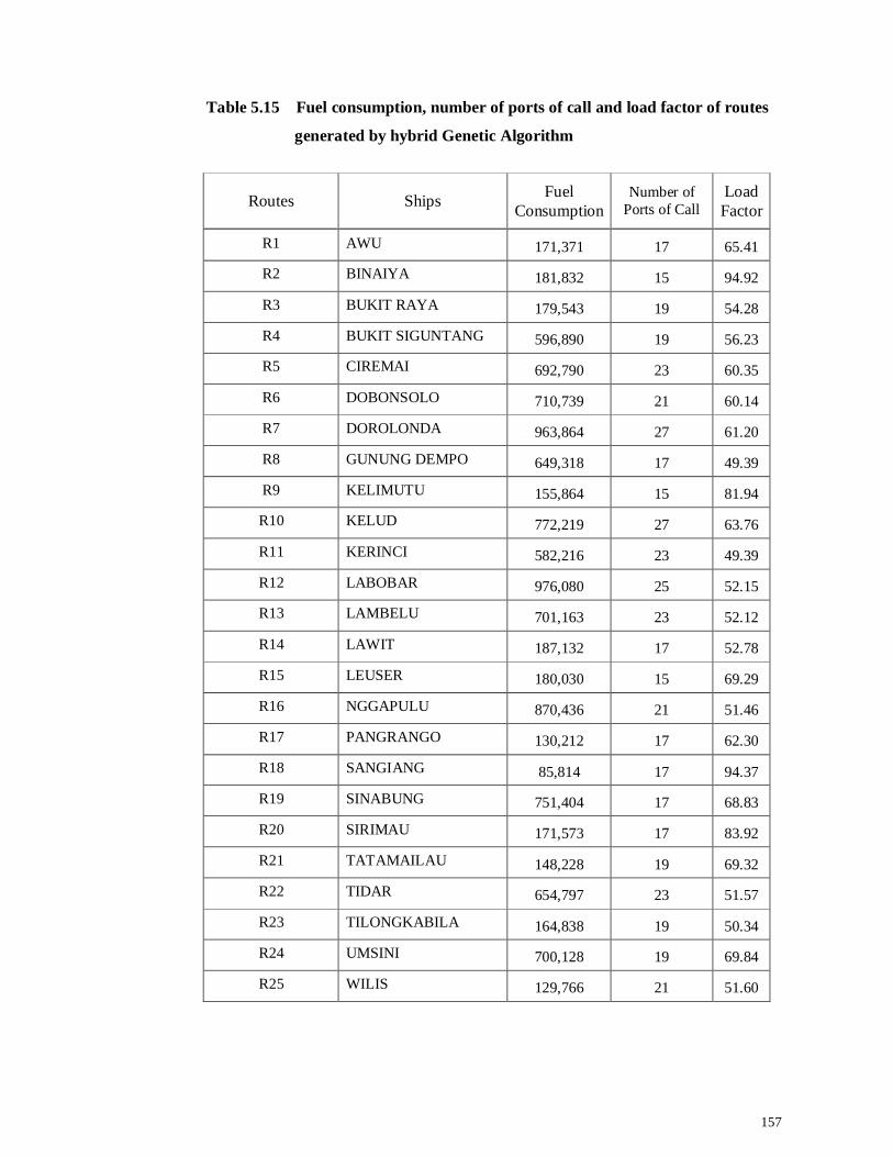
157

Table 5.15 Fuel consumption, number of ports of call and load factor of routes

generated by hybrid Genetic Algorithm

Routes Ships Fuel Consumption

Number of Ports of Call

Load Factor

R1 AWU 171,371 17 65.41

R2 BINAIYA 181,832 15 94.92

R3 BUKIT RAYA 179,543 19 54.28

R4 BUKIT SIGUNTANG 596,890 19 56.23

R5 CIREMAI 692,790 23 60.35

R6 DOBONSOLO 710,739 21 60.14

R7 DOROLONDA 963,864 27 61.20

R8 GUNUNG DEMPO 649,318 17 49.39

R9 KELIMUTU 155,864 15 81.94

R10 KELUD 772,219 27 63.76

R11 KERINCI 582,216 23 49.39

R12 LABOBAR 976,080 25 52.15

R13 LAMBELU 701,163 23 52.12

R14 LAWIT 187,132 17 52.78

R15 LEUSER 180,030 15 69.29

R16 NGGAPULU 870,436 21 51.46

R17 PANGRANGO 130,212 17 62.30

R18 SANGIANG 85,814 17 94.37

R19 SINABUNG 751,404 17 68.83

R20 SIRIMAU 171,573 17 83.92

R21 TATAMAILAU 148,228 19 69.32

R22 TIDAR 654,797 23 51.57

R23 TILONGKABILA 164,838 19 50.34

R24 UMSINI 700,128 19 69.84

R25 WILIS 129,766 21 51.60

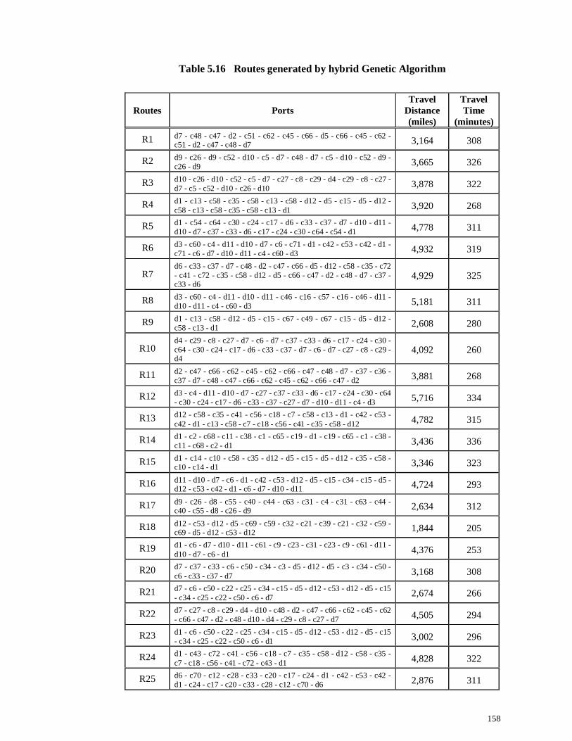
158

Table 5.16 Routes generated by hybrid Genetic Algorithm

Routes Ports Travel

Distance (miles)

Travel Time

(minutes)

R1 d7 - c48 - c47 - d2 - c51 - c62 - c45 - c66 - d5 - c66 - c45 - c62 - c51 - d2 - c47 - c48 - d7 3,164 308

R2 d9 - c26 - d9 - c52 - d10 - c5 - d7 - c48 - d7 - c5 - d10 - c52 - d9 - c26 - d9 3,665 326

R3 d10 - c26 - d10 - c52 - c5 - d7 - c27 - c8 - c29 - d4 - c29 - c8 - c27 - d7 - c5 - c52 - d10 - c26 - d10 3,878 322

R4 d1 - c13 - c58 - c35 - c58 - c13 - c58 - d12 - d5 - c15 - d5 - d12 - c58 - c13 - c58 - c35 - c58 - c13 - d1 3,920 268

R5 d1 - c54 - c64 - c30 - c24 - c17 - d6 - c33 - c37 - d7 - d10 - d11 - d10 - d7 - c37 - c33 - d6 - c17 - c24 - c30 - c64 - c54 - d1 4,778 311

R6 d3 - c60 - c4 - d11 - d10 - d7 - c6 - c71 - d1 - c42 - c53 - c42 - d1 - c71 - c6 - d7 - d10 - d11 - c4 - c60 - d3 4,932 319

R7 d6 - c33 - c37 - d7 - c48 - d2 - c47 - c66 - d5 - d12 - c58 - c35 - c72 - c41 - c72 - c35 - c58 - d12 - d5 - c66 - c47 - d2 - c48 - d7 - c37 - c33 - d6

4,929 325

R8 d3 - c60 - c4 - d11 - d10 - d11 - c46 - c16 - c57 - c16 - c46 - d11 - d10 - d11 - c4 - c60 - d3 5,181 311

R9 d1 - c13 - c58 - d12 - d5 - c15 - c67 - c49 - c67 - c15 - d5 - d12 - c58 - c13 - d1 2,608 280

R10 d4 - c29 - c8 - c27 - d7 - c6 - d7 - c37 - c33 - d6 - c17 - c24 - c30 - c64 - c30 - c24 - c17 - d6 - c33 - c37 - d7 - c6 - d7 - c27 - c8 - c29 - d4

4,092 260

R11 d2 - c47 - c66 - c62 - c45 - c62 - c66 - c47 - c48 - d7 - c37 - c36 - c37 - d7 - c48 - c47 - c66 - c62 - c45 - c62 - c66 - c47 - d2 3,881 268

R12 d3 - c4 - d11 - d10 - d7 - c27 - c37 - c33 - d6 - c17 - c24 - c30 - c64 - c30 - c24 - c17 - d6 - c33 - c37 - c27 - d7 - d10 - d11 - c4 - d3 5,716 334

R13 d12 - c58 - c35 - c41 - c56 - c18 - c7 - c58 - c13 - d1 - c42 - c53 - c42 - d1 - c13 - c58 - c7 - c18 - c56 - c41 - c35 - c58 - d12 4,782 315

R14 d1 - c2 - c68 - c11 - c38 - c1 - c65 - c19 - d1 - c19 - c65 - c1 - c38 - c11 - c68 - c2 - d1 3,436 336

R15 d1 - c14 - c10 - c58 - c35 - d12 - d5 - c15 - d5 - d12 - c35 - c58 - c10 - c14 - d1 3,346 323

R16 d11 - d10 - d7 - c6 - d1 - c42 - c53 - d12 - d5 - c15 - c34 - c15 - d5 - d12 - c53 - c42 - d1 - c6 - d7 - d10 - d11 4,724 293

R17 d9 - c26 - d8 - c55 - c40 - c44 - c63 - c31 - c4 - c31 - c63 - c44 - c40 - c55 - d8 - c26 - d9 2,634 312

R18 d12 - c53 - d12 - d5 - c69 - c59 - c32 - c21 - c39 - c21 - c32 - c59 - c69 - d5 - d12 - c53 - d12 1,844 205

R19 d1 - c6 - d7 - d10 - d11 - c61 - c9 - c23 - c31 - c23 - c9 - c61 - d11 - d10 - d7 - c6 - d1 4,376 253

R20 d7 - c37 - c33 - c6 - c50 - c34 - c3 - d5 - d12 - d5 - c3 - c34 - c50 - c6 - c33 - c37 - d7 3,168 308

R21 d7 - c6 - c50 - c22 - c25 - c34 - c15 - d5 - d12 - c53 - d12 - d5 - c15 - c34 - c25 - c22 - c50 - c6 - d7 2,674 266

R22 d7 - c27 - c8 - c29 - d4 - d10 - c48 - d2 - c47 - c66 - c62 - c45 - c62 - c66 - c47 - d2 - c48 - d10 - d4 - c29 - c8 - c27 - d7 4,505 294

R23 d1 - c6 - c50 - c22 - c25 - c34 - c15 - d5 - d12 - c53 - d12 - d5 - c15 - c34 - c25 - c22 - c50 - c6 - d1 3,002 296

R24 d1 - c43 - c72 - c41 - c56 - c18 - c7 - c35 - c58 - d12 - c58 - c35 - c7 - c18 - c56 - c41 - c72 - c43 - d1 4,828 322

R25 d6 - c70 - c12 - c28 - c33 - c20 - c17 - c24 - d1 - c42 - c53 - c42 - d1 - c24 - c17 - c20 - c33 - c28 - c12 - c70 - d6 2,876 311

159

Figure 5.17 Routes generated by hybrid Genetic Algorithm

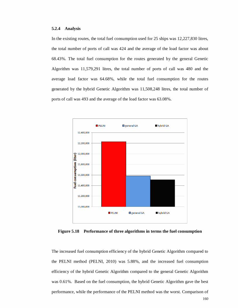
160

5.2.4 Analysis

In the existing routes, the total fuel consumption used for 25 ships was 12,227,830 litres,

the total number of ports of call was 424 and the average of the load factor was about

68.43%. The total fuel consumption for the routes generated by the general Genetic

Algorithm was 11,579,291 litres, the total number of ports of call was 480 and the

average load factor was 64.68%, while the total fuel consumption for the routes

generated by the hybrid Genetic Algorithm was 11,508,248 litres, the total number of

ports of call was 493 and the average of the load factor was 63.08%.

Figure 5.18 Performance of three algorithms in terms the fuel consumption

The increased fuel consumption efficiency of the hybrid Genetic Algorithm compared to

the PELNI method (PELNI, 2010) was 5.88%, and the increased fuel consumption

efficiency of the hybrid Genetic Algorithm compared to the general Genetic Algorithm

was 0.61%. Based on the fuel consumption, the hybrid Genetic Algorithm gave the best

performance, while the performance of the PELNI method was the worst. Comparison of

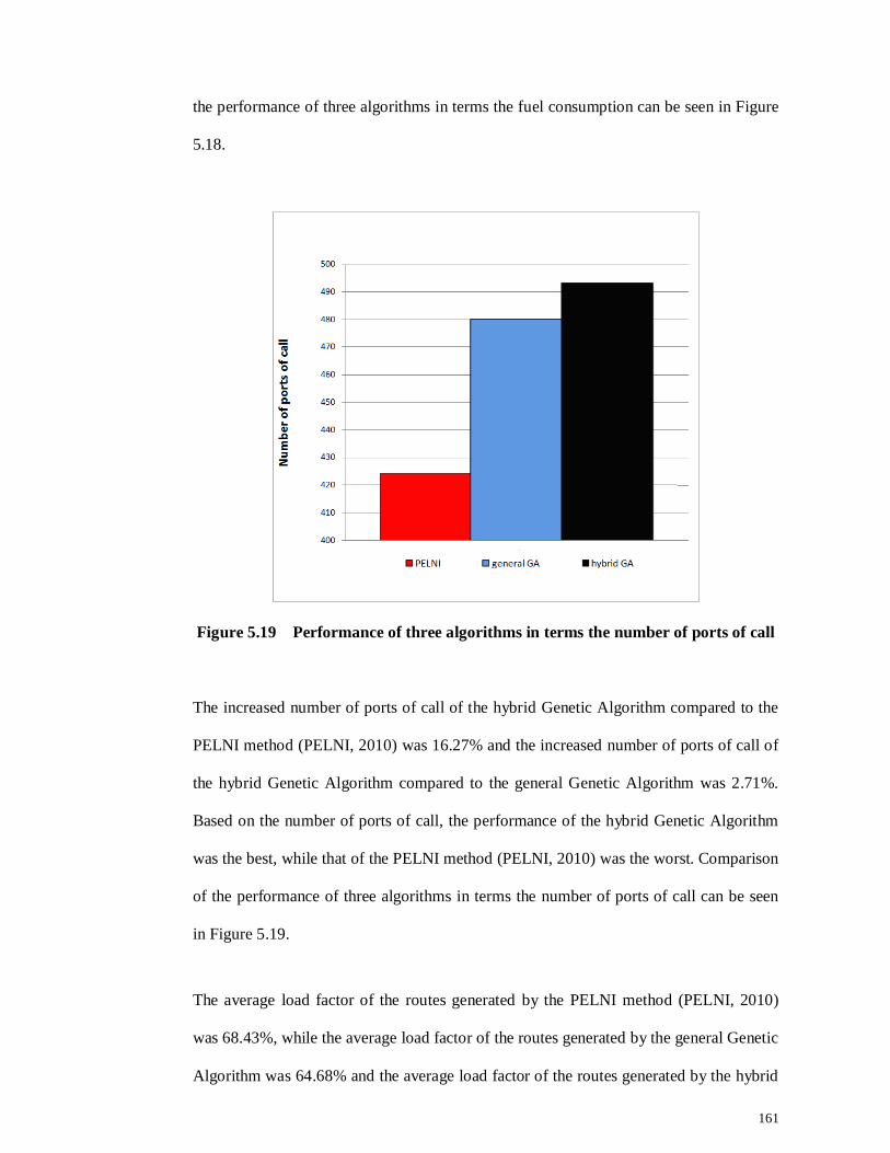
161

the performance of three algorithms in terms the fuel consumption can be seen in Figure

5.18.

Figure 5.19 Performance of three algorithms in terms the number of ports of call

The increased number of ports of call of the hybrid Genetic Algorithm compared to the

PELNI method (PELNI, 2010) was 16.27% and the increased number of ports of call of

the hybrid Genetic Algorithm compared to the general Genetic Algorithm was 2.71%.

Based on the number of ports of call, the performance of the hybrid Genetic Algorithm

was the best, while that of the PELNI method (PELNI, 2010) was the worst. Comparison

of the performance of three algorithms in terms the number of ports of call can be seen

in Figure 5.19.

The average load factor of the routes generated by the PELNI method (PELNI, 2010)

was 68.43%, while the average load factor of the routes generated by the general Genetic

Algorithm was 64.68% and the average load factor of the routes generated by the hybrid

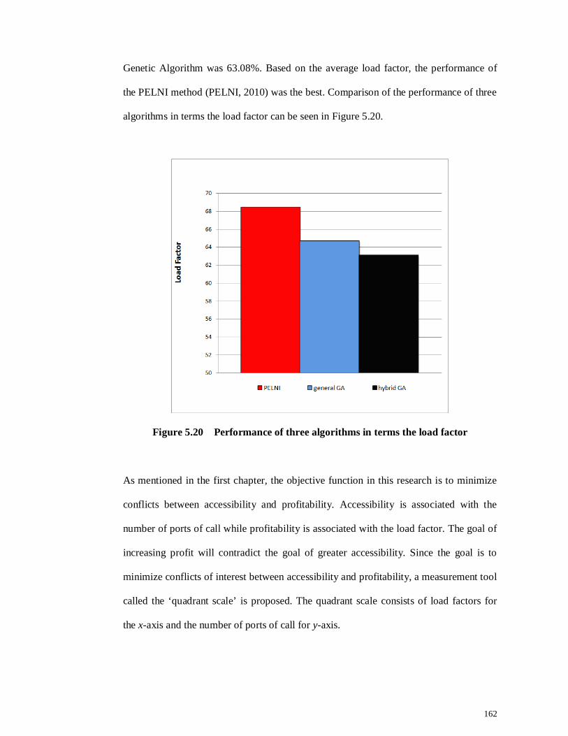
162

Genetic Algorithm was 63.08%. Based on the average load factor, the performance of

the PELNI method (PELNI, 2010) was the best. Comparison of the performance of three

algorithms in terms the load factor can be seen in Figure 5.20.

Figure 5.20 Performance of three algorithms in terms the load factor

As mentioned in the first chapter, the objective function in this research is to minimize

conflicts between accessibility and profitability. Accessibility is associated with the

number of ports of call while profitability is associated with the load factor. The goal of

increasing profit will contradict the goal of greater accessibility. Since the goal is to

minimize conflicts of interest between accessibility and profitability, a measurement tool

called the ‘quadrant scale’ is proposed. The quadrant scale consists of load factors for

the x-axis and the number of ports of call for y-axis.

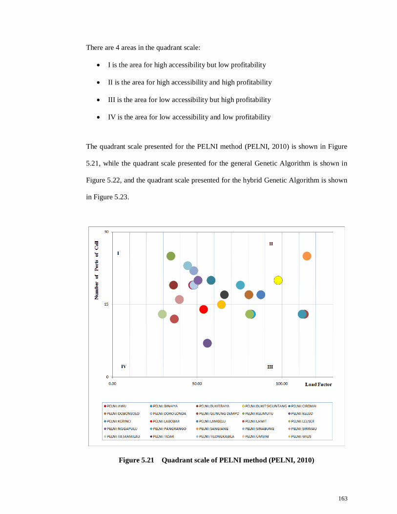
163

There are 4 areas in the quadrant scale:

I is the area for high accessibility but low profitability

II is the area for high accessibility and high profitability

III is the area for low accessibility but high profitability

IV is the area for low accessibility and low profitability

The quadrant scale presented for the PELNI method (PELNI, 2010) is shown in Figure

5.21, while the quadrant scale presented for the general Genetic Algorithm is shown in

Figure 5.22, and the quadrant scale presented for the hybrid Genetic Algorithm is shown

in Figure 5.23.

Figure 5.21 Quadrant scale of PELNI method (PELNI, 2010)

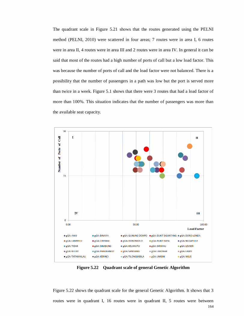
164

The quadrant scale in Figure 5.21 shows that the routes generated using the PELNI

method (PELNI, 2010) were scattered in four areas; 7 routes were in area I, 6 routes

were in area II, 4 routes were in area III and 2 routes were in area IV. In general it can be

said that most of the routes had a high number of ports of call but a low load factor. This

was because the number of ports of call and the load factor were not balanced. There is a

possibility that the number of passengers in a path was low but the port is served more

than twice in a week. Figure 5.1 shows that there were 3 routes that had a load factor of

more than 100%. This situation indicates that the number of passengers was more than

the available seat capacity.

Figure 5.22 Quadrant scale of general Genetic Algorithm

Figure 5.22 shows the quadrant scale for the general Genetic Algorithm. It shows that 3

routes were in quadrant I, 16 routes were in quadrant II, 5 routes were between

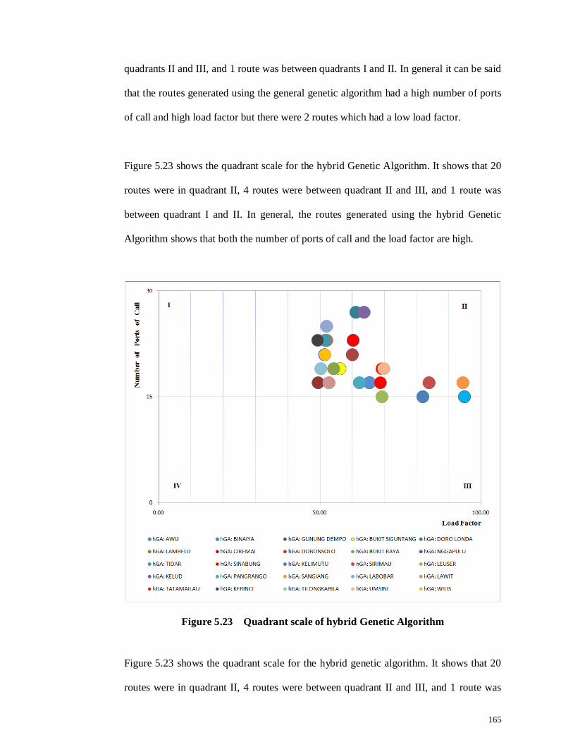
165

quadrants II and III, and 1 route was between quadrants I and II. In general it can be said

that the routes generated using the general genetic algorithm had a high number of ports

of call and high load factor but there were 2 routes which had a low load factor.

Figure 5.23 shows the quadrant scale for the hybrid Genetic Algorithm. It shows that 20

routes were in quadrant II, 4 routes were between quadrant II and III, and 1 route was

between quadrant I and II. In general, the routes generated using the hybrid Genetic

Algorithm shows that both the number of ports of call and the load factor are high.

Figure 5.23 Quadrant scale of hybrid Genetic Algorithm

Figure 5.23 shows the quadrant scale for the hybrid genetic algorithm. It shows that 20

routes were in quadrant II, 4 routes were between quadrant II and III, and 1 route was

166

between quadrant I and II. In general, the routes generated using the hybrid genetic

algorithm shows that both the number of ports of call and the load factor are high.

Based on the results presented, the best routes were generated by the hybrid Genetic

Algorithm, followed by the general Genetic Algorithm, while the PELNI method

(PELNI, 2010) showed the worst performance.

5.3 Experiment 3 - Routes Proposed

This part proposes routes which can be used to solve the routing problem of the ships in

Indonesia with greater efficiency than the existing routes. It was solved by a minimum

number of vehicles scenarios. The problem was to find optimal routes with minimum

vehicles used to serve all ports. The routes were generated by a hybrid Genetic

Algorithm, where genetic operators used were selection by roulette wheel, crossover by

multi-cut point and mutation by pair exchange. While the genetic parameters used were:

population size of 50, maximum generation of 100, crossover rate of 0.7 and mutation

rate of 0.5.

The minimum number of vehicles used to serve all ports was 17, the total fuel

consumption was 6,618,819 litres, the total number of ports of call was 319 and the

average of the load factor is about 63.31%. Table 5.17 shows the fuel consumption,

number of ports of call and load factor of routes proposed that generated by hybrid

Genetic Algorithm. Each route served by a ship where the complete routes can be seen

in Table 5.18.

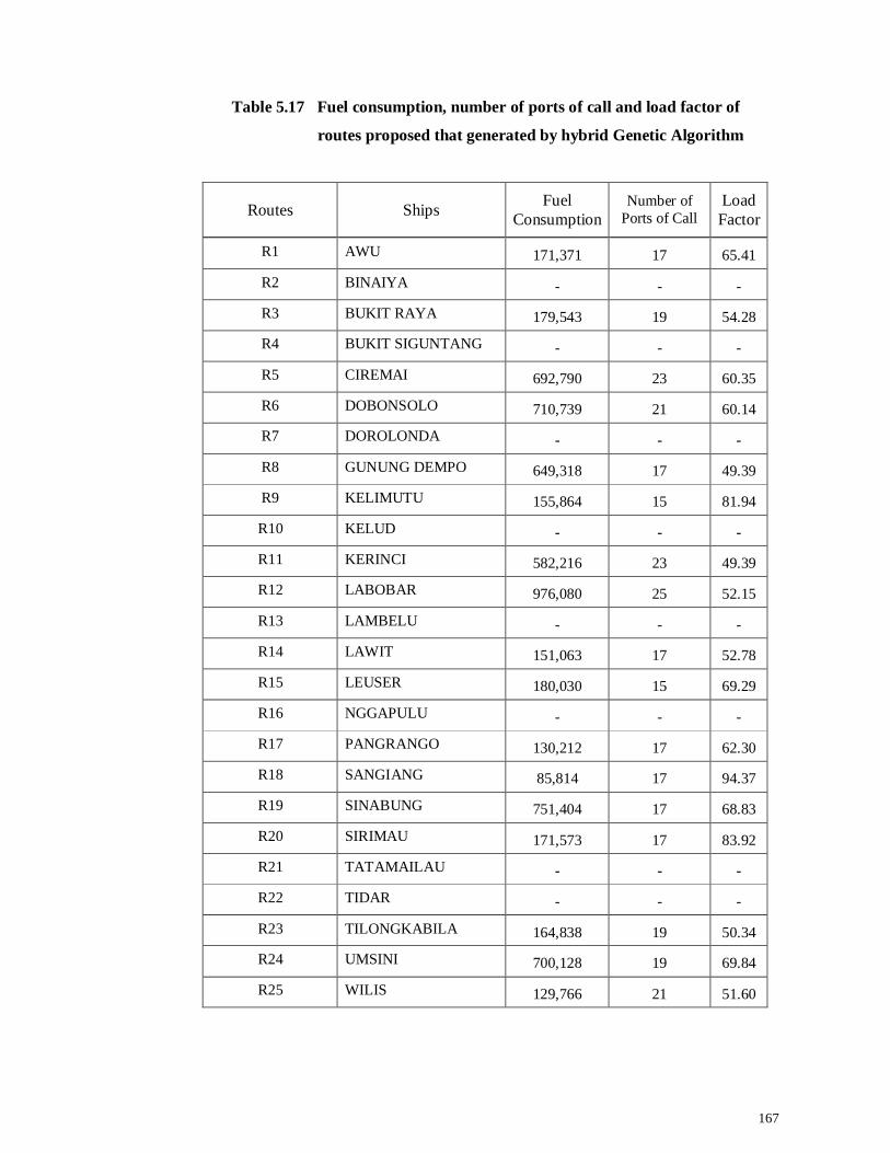
167

Table 5.17 Fuel consumption, number of ports of call and load factor of

routes proposed that generated by hybrid Genetic Algorithm

Routes Ships Fuel Consumption

Number of Ports of Call

Load Factor

R1 AWU 171,371 17 65.41

R2 BINAIYA - - -

R3 BUKIT RAYA 179,543 19 54.28

R4 BUKIT SIGUNTANG - - -

R5 CIREMAI 692,790 23 60.35

R6 DOBONSOLO 710,739 21 60.14

R7 DOROLONDA - - -

R8 GUNUNG DEMPO 649,318 17 49.39

R9 KELIMUTU 155,864 15 81.94

R10 KELUD - - -

R11 KERINCI 582,216 23 49.39

R12 LABOBAR 976,080 25 52.15

R13 LAMBELU - - -

R14 LAWIT 151,063 17 52.78

R15 LEUSER 180,030 15 69.29

R16 NGGAPULU - - -

R17 PANGRANGO 130,212 17 62.30

R18 SANGIANG 85,814 17 94.37

R19 SINABUNG 751,404 17 68.83

R20 SIRIMAU 171,573 17 83.92

R21 TATAMAILAU - - -

R22 TIDAR - - -

R23 TILONGKABILA 164,838 19 50.34

R24 UMSINI 700,128 19 69.84

R25 WILIS 129,766 21 51.60

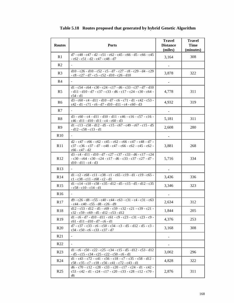
168

Table 5.18 Routes proposed that generated by hybrid Genetic Algorithm

Routes Ports Travel

Distance (miles)

Travel Time

(minutes)

R1 d7 - c48 - c47 - d2 - c51 - c62 - c45 - c66 - d5 - c66 - c45 - c62 - c51 - d2 - c47 - c48 - d7 3,164 308

R2 - - R3 d10 - c26 - d10 - c52 - c5 - d7 - c27 - c8 - c29 - d4 - c29

- c8 - c27 - d7 - c5 - c52 - d10 - c26 - d10 3,878 322

R4 - -

R5 d1 - c54 - c64 - c30 - c24 - c17 - d6 - c33 - c37 - d7 - d10 - d11 - d10 - d7 - c37 - c33 - d6 - c17 - c24 - c30 - c64 - c54 - d1

4,778 311

R6 d3 - c60 - c4 - d11 - d10 - d7 - c6 - c71 - d1 - c42 - c53 - c42 - d1 - c71 - c6 - d7 - d10 - d11 - c4 - c60 - d3 4,932 319

R7 - - R8 d3 - c60 - c4 - d11 - d10 - d11 - c46 - c16 - c57 - c16 -

c46 - d11 - d10 - d11 - c4 - c60 - d3 5,181 311

R9 d1 - c13 - c58 - d12 - d5 - c15 - c67 - c49 - c67 - c15 - d5 - d12 - c58 - c13 - d1 2,608 280

R10 - -

R11 d2 - c47 - c66 - c62 - c45 - c62 - c66 - c47 - c48 - d7 - c37 - c36 - c37 - d7 - c48 - c47 - c66 - c62 - c45 - c62 - c66 - c47 - d2

3,881 268

R12 d3 - c4 - d11 - d10 - d7 - c27 - c37 - c33 - d6 - c17 - c24 - c30 - c64 - c30 - c24 - c17 - d6 - c33 - c37 - c27 - d7 - d10 - d11 - c4 - d3

5,716 334

R13 - - R14 d1 - c2 - c68 - c11 - c38 - c1 - c65 - c19 - d1 - c19 - c65 -

c1 - c38 - c11 - c68 - c2 - d1 3,436 336

R15 d1 - c14 - c10 - c58 - c35 - d12 - d5 - c15 - d5 - d12 - c35 - c58 - c10 - c14 - d1 3,346 323

R16 - - R17 d9 - c26 - d8 - c55 - c40 - c44 - c63 - c31 - c4 - c31 - c63

- c44 - c40 - c55 - d8 - c26 - d9 2,634 312

R18 d12 - c53 - d12 - d5 - c69 - c59 - c32 - c21 - c39 - c21 - c32 - c59 - c69 - d5 - d12 - c53 - d12 1,844 205

R19 d1 - c6 - d7 - d10 - d11 - c61 - c9 - c23 - c31 - c23 - c9 - c61 - d11 - d10 - d7 - c6 - d1 4,376 253

R20 d7 - c37 - c33 - c6 - c50 - c34 - c3 - d5 - d12 - d5 - c3 - c34 - c50 - c6 - c33 - c37 - d7 3,168 308

R21 - - R22 - - R23 d1 - c6 - c50 - c22 - c25 - c34 - c15 - d5 - d12 - c53 - d12

- d5 - c15 - c34 - c25 - c22 - c50 - c6 - d1 3,002 296

R24 d1 - c43 - c72 - c41 - c56 - c18 - c7 - c35 - c58 - d12 - c58 - c35 - c7 - c18 - c56 - c41 - c72 - c43 - d1 4,828 322

R25 d6 - c70 - c12 - c28 - c33 - c20 - c17 - c24 - d1 - c42 - c53 - c42 - d1 - c24 - c17 - c20 - c33 - c28 - c12 - c70 - d6

2,876 311

169

Figure 5.24 Routes proposed for minimum ships scenarios that generated by hybrid Genetic Algorithm

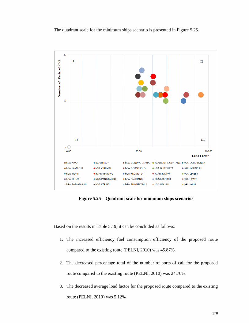
170

The quadrant scale for the minimum ships scenario is presented in Figure 5.25.

Figure 5.25 Quadrant scale for minimum ships scenarios

Based on the results in Table 5.19, it can be concluded as follows:

1. The increased efficiency fuel consumption efficiency of the proposed route

compared to the existing route (PELNI, 2010) was 45.87%.

2. The decreased percentage total of the number of ports of call for the proposed

route compared to the existing route (PELNI, 2010) was 24.76%.

3. The decreased average load factor for the proposed route compared to the existing

route (PELNI, 2010) was 5.12%

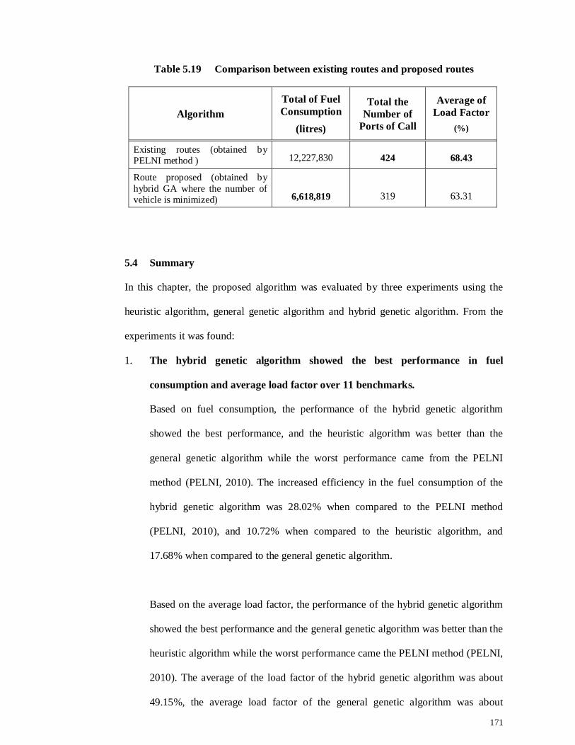
171

Table 5.19 Comparison between existing routes and proposed routes

Algorithm Total of Fuel Consumption

(litres)

Total the Number of

Ports of Call

Average of Load Factor

(%)

Existing routes (obtained by PELNI method ) 12,227,830 424 68.43

Route proposed (obtained by hybrid GA where the number of vehicle is minimized) 6,618,819 319 63.31

5.4 Summary

In this chapter, the proposed algorithm was evaluated by three experiments using the

heuristic algorithm, general genetic algorithm and hybrid genetic algorithm. From the

experiments it was found:

1. The hybrid genetic algorithm showed the best performance in fuel

consumption and average load factor over 11 benchmarks.

Based on fuel consumption, the performance of the hybrid genetic algorithm

showed the best performance, and the heuristic algorithm was better than the

general genetic algorithm while the worst performance came from the PELNI

method (PELNI, 2010). The increased efficiency in the fuel consumption of the

hybrid genetic algorithm was 28.02% when compared to the PELNI method

(PELNI, 2010), and 10.72% when compared to the heuristic algorithm, and

17.68% when compared to the general genetic algorithm.

Based on the average load factor, the performance of the hybrid genetic algorithm

showed the best performance and the general genetic algorithm was better than the

heuristic algorithm while the worst performance came the PELNI method (PELNI,

2010). The average of the load factor of the hybrid genetic algorithm was about

49.15%, the average load factor of the general genetic algorithm was about

172

46.80%, the average load factor of the heuristic algorithm was about 23.52%, and

the average load factor of the PELNI method (PELNI, 2010) was about 4.48%.

2. The hybrid genetic algorithm showed the best performance in fuel

consumption and number of ports of call in solving the routing problems of

the ship in Indonesia.

Based on fuel consumption, the performance of the hybrid genetic algorithm

showed the best performance while the worst performance was from the PELNI

method (PELNI, 2010). The increased efficiency in the fuel consumption of the

hybrid genetic algorithm was 5.88% when compared to the PELNI method

(PELNI, 2010), and 0.61% when compared to the general genetic algorithm. Based

on the number of ports of call, the performance of the hybrid genetic algorithm

showed the best performance while the worst performance came the PELNI

method. The increased number of ports of call of the hybrid genetic algorithm was

16.27% when compared to the PELNI method (PELNI, 2010), and 2.71% when

compared to the general genetic algorithm.

3. The routes produced by the hybrid genetic algorithm for the minimum

number of vehicles scenario were 45.87% more efficient with regard to fuel

consumption than the existing routes by the PT. PELNI (PELNI, 2010).

4. Hence, the hybrid genetic algorithm showed the best overall performance

When the quadrant scale was applied for the analysis of the performances of the

algorithms, hybrid genetic algorithm clearly outperformed the others.

Therefore, it was concluded conclude that the new hybrid algorithm is far superior to the

current available method for the research problem discussed.

173

CHAPTER 6 CONCLUSIONS AND FUTURE WORK

This chapter summarizes and concludes our research into solving the vehicle routing

problem (VRP), as discussed. Several recommendations for future work and algorithm

improvements are also included.

6.1 Research Summary

The general vehicle routing problem consists of determining several vehicle routes, with

minimum cost, to serve a set of customers. Each customer is required to be visited only

once by one vehicle. Typically, vehicles are homogeneous and have the same capacity

restriction. This research used heuristics and metaheuristics to solve the ship routing

problem. There are four vehicle routing problem variants, which are similar to the ship

routing problem, namely the multi-depot vehicle routing problem (MDVRP), the

heterogeneous fleet vehicle routing problem (HVRP), the site dependent capacitated

vehicle routing problem (SDCVRP) and the asymmetric vehicle routing problem

(AVRP).

The vehicle fleet is a mixture of different vehicle types. Ships are of different capacities,

speeds and costs. There are two types of constraints, namely; soft constraints and hard

constraints.

1. Soft constraints

There are two soft constraints for the ship routing problem i.e. ship draft and sea

depth, and load factor. Soft constraints are dealt with by imposing a penalty.

174

2. Hard constraints

There are three hard constraints for the ship routing problem i.e, travel time, travel

distance, and a route included due to the necessity of having at least one fuel port

within the route. Hard constraints are dealt with by removing unfeasible routes.

Vehicle routing problem is a general combinatorial optimization and is an NP-hard

problem. This means that it is not guaranteed that there is a known algorithm that solves

all cases to optimality in a reasonable execution time. As this problem cannot be solved

by optimal (exact) methods in practice, heuristic and metaheuristics are used. In this

research, a heuristic algorithm (based on the next nearest neighbour concept) was

modified and applied to the case study.

We implemented a new model for chromosome where the length of a chromosome

depends on the number of ships. Each ship is represented as a sub-chromosome where

each sub-chromosome consists of 14 genes. A sub-chromosome consists of Q-arm, P-

arm, and two centromeres. The 1st and 10th genes contain a value that refers to the fuel

port. The 2nd - 9th are called Q-arm, while the 11th - 14th are called P-arm. Q-arm and

P-arm contain a value that refers to the customer’s port.

The crossover method is based on a modified multi-cut point crossover. The crossover is

done by exchanging Q-arm and P-arm between two parents’ chromosomes. Pairs

exchange mutation is applied to P-arm. After recombination, all chromosomes are

checked to ensure that the travel time constraint and travel distance is not violated.

When a chromosome violates these constraints, it is repaired. During the repairing

process, the ports that are served more than once are deleted.

175

The objectives that can be used to analyse the performance of public transportation

routes that are owned and operated by government are fuel consumption, number of

ports of call, and load factor. Since the objective of solving our problem is how to

determine the combination of routes that give minimum fuel consumption, maximum

number of ports of call and maximum load factor by satisfying a number of

predetermined constraints, it is difficult to calculate one best solution.

Hence, we used a measurement tool known as a quadrant scale. The quadrant scale

consists of load factor for the x axis and number of ports of call for the y axis. There are

4 areas in the quadrant scale:

I is the area used for high accessibility and low profitability

II is the area used for high accessibility and high profitability

III is the area used for low accessibility and high profitability

IV is the area used for low accessibility and low profitability

Based on the quadrant scale analysis:

The quadrant scale for the routes generated using the PELNI method are

scattered in four areas i.e., 7 routes in area I, 6 routes in area II, 4 routes in area

III, and 2 routes in area IV. Most of the routes have a high number of ports of

call, but they have a low load factor. This situation is due to the number of ports

of call and the load factor not being balanced. There is a possibility that the

number of passengers in a path is low but the port is served more than twice in

one week.

The quadrant scale for the general Genetic Algorithm shows that 3 routes are in

quadrant I, 16 routes are in quadrant II, 5 routes are between quadrants II and III,

and 1 route is between quadrants I and II. The routes generated using the general

176

Genetic Algorithm have a high number of ports of call and a high load factor but

there are 2 routes that have a low load factor.

The quadrant scale for the hybrid Genetic Algorithm shows that 20 routes are in

quadrant II, 4 routes are between quadrants II and III, and 1 route is between

quadrants I and II. Thus, the routes generated using the hybrid Genetic Algorithm

show that both the number of ports of call and the load factor are high.

Based on the results presented in Chapter 5, the hybrid Genetic Algorithm shows the

ability to obtain a better solution to the ship routing problem than the PELNI method and

the general Genetic Algorithm. All of the results can be summarized as follows:

The increased fuel consumption efficiency of the hybrid Genetic Algorithm

compared to the PELNI method is 5.88 %; and the increased fuel consumption

efficiency of the hybrid Genetic Algorithm, compared to the general Genetic

Algorithm, is 0.61%.

The increased number of ports of call of the hybrid Genetic Algorithm compared

to the PELNI method is 16.27%; and the increased number of ports of call of the

hybrid Genetic Algorithm compared to the general Genetic Algorithm, is 2.71%.

The decreased load factor of the hybrid Genetic Algorithm compared to the

PELNI method is approximately 3.75%; and the decreased load factor of the

hybrid Genetic Algorithm compared to the general Genetic Algorithm, is

approximately 1.60%.

We proposed an optimum route, where 17 vehicles are used to serve all ports. The

comparison of the existing routes and the proposed routes is summarized as follows:

4. Total fuel consumption used to serve all ports in the routes proposed is 6,618,819

litres while the total fuel consumption in the existing routes is 12,227,830 liters.

177

Fuel consumption efficiency is increased by approximately 45.87% compared to

the existing routes.

5. The total the number of ports of call in the routes proposed is 319 while the total

number of ports of call in the existing routes is 424. The number of ports of call

is decreased by 24.76% compared to the existing routes.

6. The load factor average of the routes proposed is 63.31%, while the load factor

average of the existing routes is 68.43%. Therefore, load factor average

decreased by 5.21% compared to the existing routes.

6.2 Contribution

The following are some of the contributions to this study:

Identification of the nature of the ship routing problem in Indonesian waters.

A ship routing problem consists of four different Vehicle Routing Problem (VRP)

variants, namely the multi-depot vehicle routing problem (MDVRP), the

heterogeneous fleet vehicle routing problem (HVRP), the site dependent

capacitated vehicle routing problem (SDCVRP) and the asymmetric vehicle

routing problem (AVRP).

New chromosome model

A chromosome in the hybrid Genetic Algorithm is represented as a number of sub-

chromosomes. Each sub-chromosome consists of Q-arm, P-arm and two

centromeres. The 1st and 10th genes (known as centromere) contain values that

refer to the fuel port. The 2nd to the 9th genes are known as the Q-arm and the

11th to the 14th genes are known as the P-arm. Q-arm and P-arm both contain

values that refer to the customer’s port.

178

Method to solve the ship routing problem.

o The heuristic method is which ‘cluster first and route second’.

Three phases are included in this method i.e. clustering, assigning of vehicle,

and finding the best routes by combining feasible solutions.

(i) Phase I: Clustering

Routes are clustered in order to solve the constraint based on problems of

travel time and travel distance allowed for each route. Travel time is less

than or equal to the maximum travel time allowed and travel distance is less

than or equal to the maximum travel distance allowed. The output is a

feasible route set for the solution candidate.

(ii) Phase II: Assigning a vehicle

Vehicles are assigned in a cluster to ensure that each route has at least one

fuel port (the route is removed if this condition is violated) During this

phase, fuel consumption is calculated with a penalty α imposed if the ship’s

draft is equal to or greater than the sea depth; penalty β is imposed for the

load factor conditions; and penalty γ is imposed for the number of ports of

call condition.

(iii) Phase III: Finding the best routes

A robust algorithm was developed based on the maximum-insertion concept

where a heuristic model with a maximum-insertion concept was modified,

where the objective was to successively insert a route within the best

combination of routes with the minimum fuel consumption.

o Hybrid Genetic Algorithm

A hybrid genetic algorithm (hybrid Genetic Algorithm) was proposed to

improve the performance of the general Genetic Algorithm. The differences

between the general Genetic Algorithm and the hybrid Genetic Algorithm

are as follows:

179

(i) Initial population

The initial population of the general Genetic Algorithm is generated

randomly while in the hybrid Genetic Algorithm is generated using a

random mix with the nearest neighbour concept. The centromere

generated is random, while the Q-arm and the P-arm are generated

using the nearest neighbour.

(ii) Improvement procedure

This procedure compares the best parent and offspring fitness’s, and

the chromosome with the best fitness is perpetuated into the next

generation.

6.3 Limitations

There are several limitations of this study:

Determination of penalty for soft constraints is only done by forecasting.

Two soft constraint penalty values cannot be precisely determined, namely:

i. Load factor

ii. Number of ports of call

Determinations of penalty values for these soft constraints affect the accuracy of

achievement of the objective function. If the penalty values can be determined

precisely, then a comparison between the three objectives would be more

appropriate.

Scheduling issues of routes are not addressed in detail.

180

6.4 Further Work

There is a need for future works to address the limitations listed above:

Determination of the penalty’s value

Penalty values can be made more precise, so that a comparison between the three

objectives can be made more accurately.

Two ships anchored in the same port at the same time

Two ships can be anchored in the same port at the same time. Some passengers

may change their journey to another route. If this facility is available, then

travelling times can be reduced for passengers.

6.5 Conclusion

From the detailed discussion contained within this thesis, we have shown that the

objective of our research has been achieved. In doing so, we have also contributed a new

method to solve the ship routing problem discussed.

181

BIBLIOGRAPHY

Archetti, C., Feillet, D., Gendreau, M., & Speranza, M. (2010). Complexity of the VRP

and SDVRP. Transportation Part C, 1-10.

Baldacci, R., Battarra, M., & Vigo, D. (2008). Routing a heterogeneous fleet of vehicles.

The Vehicle Routing Problem: Latest Advances and New Challenges, 43, 3-27.

Beasley, J. E. (1983). Route-first cluster-second methods for vehicle routing. Omega, 11,

403-408.

Bertsimas, D. J., & Simchi-Levi, D. (1996). A new generation of vehicle routing

research: Robust algorithms addressing uncertainty. Operations Research (44),

286-304.

Bianchi, L. (2006). Ant colony optimization and local search for the probabilistic

traveling salesman problem: a case study in stochastic combinatorial

optimization. Unpublished PhD’s thesis, Universite Libre de Bruxelles, Belgium.

Bonyadi, M. R., Azghadi, M. R., & Shah-Hosseini, H. (2008). Population-based

optimization algorithms for solving the travelling salesman problem. In F. Greco

(Ed.), Travelling Salesman Problem. Vienna: I-Tech.

Brandão, J. (2011). A tabu search algorithm for the heterogeneous fixed fleet vehicle

routing problem. Computers & Operations Research, 38 (1), 140-151.

Branke, J., & Guntsch, M. (2004). Solving the probabilistic TSP with ant colony

optimization. Journal of Mathematical Modelling and Algorithms, 3 (4), 403-

428.

Bullnheimer, B., Hartl, R. F., & Strauss, C. (1999). An improved ant system algorithm

for the vehicle routing problem. Annals of Operations Res., 89, 319-328.

Chao, I. M., Golden, B., & Wasil, E. (1998). A new algorithm for the site-dependent

vehicle routing problem. Advances in Computational and Stochastic

Optimization, Logic Programming, and Heuristic Search: Interfaces in

182

Computer Science and Operations Research, 301-312.

Choi, E., & Tcha, D. W. (2007). Column generation approach to the heterogeneous fleet

vehicle routing problem. Computers & Operations Research 34(7), 2080-2095.

Choi, I. C., Kim, S. I., & Kim, H.-S. (2003). A genetic algorithm with a mixed region

search for the asymmetric travelling salesman problem. Computers & Operations

Research, 30 (5), 773-786.

Christiansen, M. Fagerholt, K., Nygreen, B & Ronen, D. (2005). Transportation. In C.

Barnhart And G. Laporte (Eds.), Operations research and management science.

North-Holland, Amsterdam.

Christofides, N., Mingozzi, A., & Toth, P. (1979). The vehicle routing problem. In N.

Christofides, Mingozzi, A., Toth, P., & Sandi, C. (Series Eds.), Combinatorial

Optimization. North-Holland, Amsterdam.

Clarke, G., & Wright, J. W. (1964). Scheduling of vehicles from a central depot to a

number of delivery points. Operations Research 12 (4), 568-581.

Colorni, A., Dorigo, M., & Maniezzo, V. (1991). Distributed Optimization by Ant

Colonies. First European Conference on Artificial Life, 134-142.

Cordeau, J. F., Gendreau, M., & Laporte, G. (1997). A Tabu Search heuristic for

periodic and multi-depot vehicle routing problems. Networks, 30 (2), 105-119.

Cordeau, J. F., & Laporte, G. (2001). A Tabu Search algorithm for the site dependent

vehicle routing problem with time windows. INFOR, 39 (3), 292-298.

Dantzig, G. B., & Ramser, J. H. (1959). The truck dispatching problem. Management

Science, 6 (1), 80-91.

Dondo, R., & Cerdá, J. (2007). A cluster-based optimization approach for the multi-

depot heterogeneous fleet vehicle routing problem with time windows. European

Journal of Operational Research, 176 (3), 1478-1507.

Dorigo, M., & Stutzle, T. (2004). Ant colony optimization. Massachusetts. London: the

MIT Press Cambridge.

183

Falkenauer, E. (1996). A hybrid grouping genetic algorithm for bin packing. Journal of

Heuristics, 2 (1), 5-30.

Fuellerer, G., Doerner, K. F., Hartl, R. F., & Iori, M. (2009). Ant colony optimization of

the two-dimensional loading vehicle routing problem. Computers & Operations

Research, 36 (3), 655-673.

Gen, M., & Cheng, R. (1999). Genetic algorithms and engineering optimization. New

York: Wiley-Interscience.

Gendreau, M., Hertz, A., & Laporte, G. (1994). A tabu search heuristic for the vehicle

routing problem. Management Science, 40, 1276-1290.

Gendreau, M., Laporte, G., Musaraganyi, C., & Taillard, E. D. (1999). A tabu search

heuristic for the heterogeneous fleet vehicle routing problem. Computers &

Operations Research, 26, 1153-1173.

Gendreau, M., M. Iori, Laporte, G., & Martello, S. (2006). A tabu search algorithm for a

routing and container loading problem. Transportation Science, 40 (3), 342-350.

Gillett, B. E., & Miller, L. R. (1974). A heuristic algorithm for the vehicle-dispatch

problem. Operations Research 21, 340-349.

Ginting, F. (2003). Kajian efektifitas jaringan rute angkutan penumpang laut PT PELNI

di Indonesia. Unpublished master’s thesis, Institute of Technology Bandung,

Indonesia.

Glover, F. (1990). Tabu search II. ORSA Journal on Computing, 2 (1), 4-32.

Goldberg, D. E. (1989). Genetic algorithms in search, optimization, and machine

learning. New York: Addison-Wesley.

Greco, F., & Gerace, I. (2008). The symmetric circulant traveling salesman problem. In

F. Greco (Ed.), Travelling Salesman Problem. Vienna: I-Tech.

Haimovich, M., & Kan, A. H. G. R. (1985). Bounds and heuristics for capacitated

routing problems. Mathematics of Operations Research, 10, 527-542.

Ho, W., Ho, G. T., Ji, P., & Lau, H. C. W. (2008). Hybrid genetic algorithm for the

184

multi-depot vehicle routing problem. Engineering Applications of Artificial

Intelligence 21 (4), 548-557.

Ho, W., & Ji, P. (2003). Component scheduling for chip shooter machines: a hybrid

genetic algorithm approach. Computers & Operations Research, 30 (14), 2175-

2189.

Japan International Corporation Agency. (2004). Study on the development of domestic

sea transportation and maritime in the Republic of Indonesia. Jakarta: Author.

Jeon, G., Leep, H. R., & Shim, J. Y. (2007). A vehicle routing problem solved by using a

hybrid genetic algorithm. Computers & Industrial Engineering, 53 (4), 680-692.

Kirkpatrick, S., Gelatt, C. D., & Vecchi, M. P. (1983). Optimization by simulated

annealing. Science, 220 (4598), 671-680.

Kuo, Y. (2010). Using simulated annealing to minimize fuel consumption for the time-

dependent vehicle routing problem. Computers & Industrial Engineering, 59,

157-165.

Laporte, G., & Semet, F. (2002). Classical heuristics for the capacitated VRP. In P. Toth,

Vigo, D (Series Ed.) The Vehicle Routing Problem. Philadelphia: SIAM

Monographs on Discrete Mathematics and Applications.

Lau, H. C. W., Chan, T. M., Tsui, W. T., & Pang, W. K. (2010). Application of genetic

algorithms to solve the multidepot vehicle routing problem. IEEE Transactions

on Automation Science and Engineering, 7 (2), 383-392.

Li, X. Y., Tian, P., & Leung, S. C. H. (2009). An ant colony optimization metaheuristic

hybridized with tabu search for open vehicle routing problems. Journal of the

Operational Research Society, 60 (7), 1012-1025.

Lin, S. (1965). Computer solutions of the travelling salesman problem. Bell System

Technical Journal, 44, 2245-2269.

Lin, S.-W., Lee, Z.-J., Ying, K.-C., & Lee, C.-Y. (2009). Applying hybrid meta-

heuristics for capacitated vehicle routing problem. Expert Systems with

185

Applications, 36 (2), 1505-1512.

Liu, Y. H. (2008). Solving the probabilistic travelling salesman problem based on

genetic algorithm with queen selection scheme. In F. Greco (Ed.), Travelling

Salesman Problem. Vienna: I-Tech.

Liu, Y. H., Jou, R. C., & Wang, C. J. (2004). Genetic algorithms for the probabilistic

traveling salesman problem. Journal of E-logistics, 77-82.

Liu. S., Huang, W., & Ma. H. (2009). An effective genetic algorithm for the fleet size

and mix vehicle routing problems. Transportation Research Part E 45 434-445.

Lupsa, L., Chiorean, I., RaduLupsa, & Neamtiu, L. (2010). Some special traveling

salesman problems with applications in health economics. In D. Davendra (Ed.),

Traveling Salesman Problem, Theory and Applications. Vienna: I-Tech..

Matai, R., Singh, S. P., & Mittal, M. L. (2010). Traveling salesman problem: an

overview of applications, formulations, and solution approaches. In D. Davendra

(Ed.), Traveling Salesman Problem, Theory and Applications. Vienna: I-Tech.

Mazzeo, S., & Loiseau, I. (2004). An Ant Colony Algorithm for the Capacitated Vehicle

Routing. Electronic Notes in Discrete Mathematics, 18, 181-186.

Nag, B., Golden, B. L., & Assad, A. (1988). Vehicle routing with site dependencies.

Vehicle Routing: Methods and Studies, 149-159.

Nagata, Y., & Bräysy, O. (2009). Edge assembly-based memetic algorithm for the

capacitated vehicle routing problem. Networks, 54 (4), 205-215.

Nagy, G., & Salhi, S. d. (2005). Heuristic algorithms for single and multiple depot

vehicle routing problems with pickups and deliveries. European Journal of

Operational Research, 162 (1), 126-141.

Novoa, C., Berger, R., Linderoth, J., & Storer, R. (2006). A set-partitioning-based model

for the stochastic vehicle routing problem (pp. 1-30): Lehigh University Press.

Ochi, L. S., Vianna, D. S., Drummond, L., & Victor, A. (1998). A parallel evolutionary

algorithm for the vehicle routing problem with heterogeneous fleet. Future

186

Generation Computation Systems, 14 (5), 285-292.

Osman, I. H. (1993). Metastrategy simulated annealing and tabu search algorithms for

the vehicle routing problem. Annals of Operations Research, 41 (4), 421-451.

PELNI. (2008). Laporan tahunan 2008. Jakarta: Indonesia Government Printing Office.

PELNI. (2010). Laporan tahunan 2010. Jakarta: Indonesia Government Printing Office.

Penna, P. H. V., Subramanian, A., & Ochi, L. S. (2011). An iterated local search

heuristic for the heterogeneous fleet vehicle routing problem. Journal of

Heuristics, 1-32.

PERTAMINA. (2008). Panduan Pelayanan BBM Bunker. Jakarta: Indonesia

Government Printing Office.

Pertiwi, I. (2005). Pendekatan pemecahan berbasis set covering heuristik untuk

pemecahan masalah penentuan rute dan penugasan kapal. Unpublished Ph.D’s

thesis, Institute of Technology Bandung, Indonesia.

Pessoa, A., Uchoa, E., & Aragão, M. P. d. (2009). A robust branch-cut-and-price

algorithm for the heterogeneous fleet vehicle routing problem. Networks, 54 (4),

167-177.

Prins, C. (2002). Eficient heuristics for the heterogeneous fleet multitrip VRP with

application to a large-scale real case. Journal of Mathematical Modelling and

Algorithms 1 (2), 135-150.

Prins, C. (2009). Two memetic algorithms for heterogeonous fleet vehicle routing

problems. Engineering Applications of Artificial Intelligence, 22 (6), 916-928.

Reinelt, G. (1994). The traveling salesman: computational solutions for TSP

applications. Berlin, Heidelberg: Springer-Verlag.

Renaud, J., Laporte, G., & Boctor, F. F. (1996). A Tabu Search heuristic for the multi-

depot vehicle routing problem. Computers & Operations Research, 23 (3), 229-

235.

Salhi, S., & Sari, M. (1997). A multi-level composite heuristic for the multi-depot

187

vehicle fleet mix problem. European Journal of Operational Research, 103 (1),

95-112.

Silver, E. A., Vidal, R. V., & Werra, D. d. (1980). A tutorial on heuristic methods.

European Journal of Operational Research, 5, 153-162.

Statistik. (2010). Statistik penduduk Indonesia tahun 2010. Jakarta: Indonesia

Government Printing Office.

Subramanian, A., Penna, P. H. V., Uchoa, E., & Ochi, L. S. (2012). A hybrid algorithm

for the heterogeneous fleet vehicle routing problem. European Journal of

Operational Research, 221, 285-295.

Taillard, E. D. (1999). A heuristic column generation method for the heterogeneous fleet

VRP. RAIRO - Operations Research, 33 (1), 1-14.

Tarantilis, C. D., Kiranoudis, C. T., & Vassiliadis, V. S. (2003). A list-based threshold

accepting metaheuristic for the heterogeneous fixed fleet vehicle routing

problem. Journal of the Operational Research Society, 54 (1), 65-71.

Tarantilis, C. D., Kiranoudis, C. T., & Vassiliadis, V. S. (2004). A threshold accepting

metaheuristic for the heterogeneous fixed fleet vehicle routing problem. Journal

of the Operational Research Society 152, 148-158.

Wei, J. D. (2008). Approaches to the travelling salesman problem using evolutionary

computing algorithms In F. Greco (Ed.), Travelling Salesman Problem (pp. 202).

Vienna, Austria: I-Tech.

Wren, A. (1971). Computers in Transport Planning and Operation. London: Ian Allan.

Wren, A., & Holliday, A. (1972). Computer scheduling of vehicles from one or more

depots to a number of delivery points. Operational Research Quarterly 23, 333-

344.

Yaman, H. (2006). Formulations and valid inequalities for the heterogeneous vehicle

routing problem. Mathematical Programming 106 (2), 365-390.

Zachariadis, E. E., Tarantilis, C. D., & Kiranousdis, C. T. (2009). A guided tabu search

188

for the vehicle routing problem with two-dimensional loading constraints.

European Journal of Operational Research, 195 (3), 729–743.

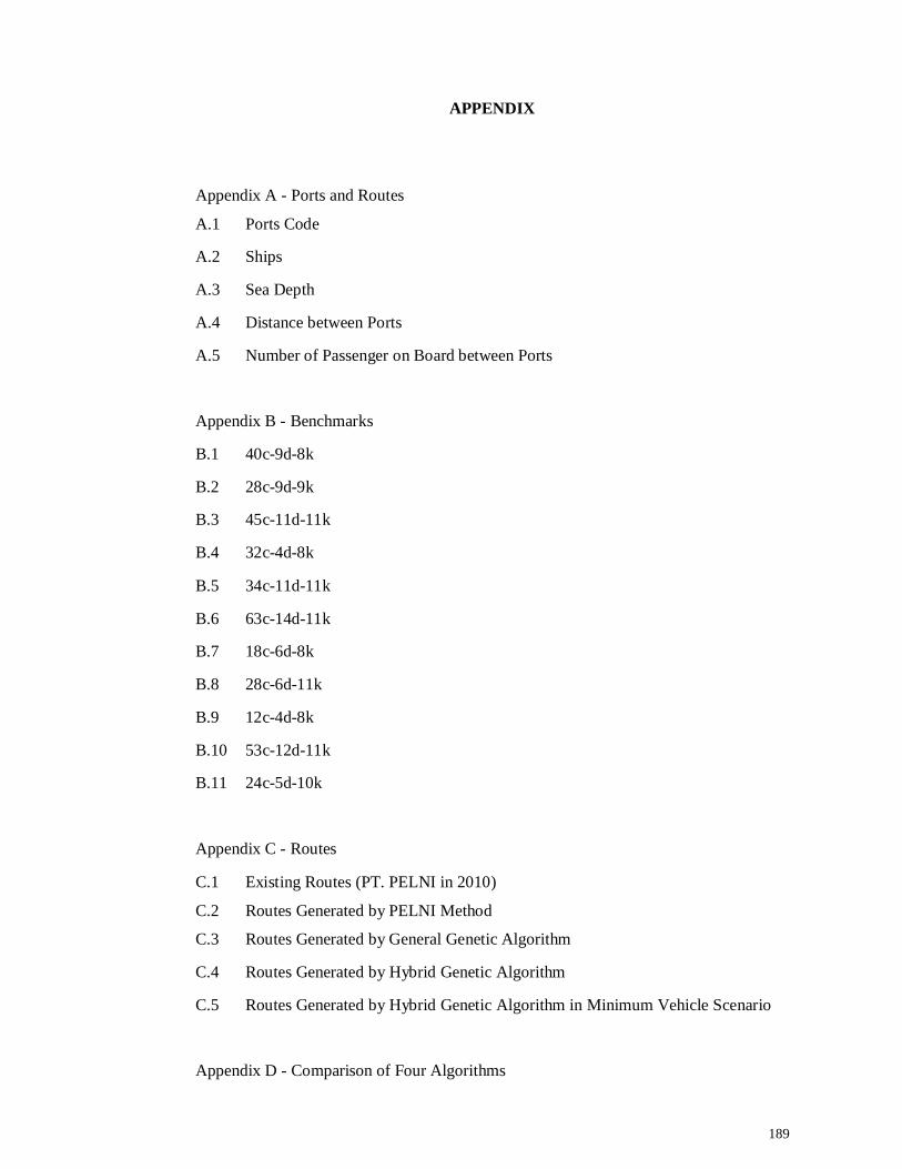
189

APPENDIX

Appendix A - Ports and Routes

A.1 Ports Code

A.2 Ships

A.3 Sea Depth

A.4 Distance between Ports

A.5 Number of Passenger on Board between Ports

Appendix B - Benchmarks

B.1 40c-9d-8k

B.2 28c-9d-9k

B.3 45c-11d-11k

B.4 32c-4d-8k

B.5 34c-11d-11k

B.6 63c-14d-11k

B.7 18c-6d-8k

B.8 28c-6d-11k

B.9 12c-4d-8k

B.10 53c-12d-11k

B.11 24c-5d-10k

Appendix C - Routes

C.1 Existing Routes (PT. PELNI in 2010)

C.2 Routes Generated by PELNI Method

C.3 Routes Generated by General Genetic Algorithm

C.4 Routes Generated by Hybrid Genetic Algorithm

C.5 Routes Generated by Hybrid Genetic Algorithm in Minimum Vehicle Scenario

Appendix D - Comparison of Four Algorithms

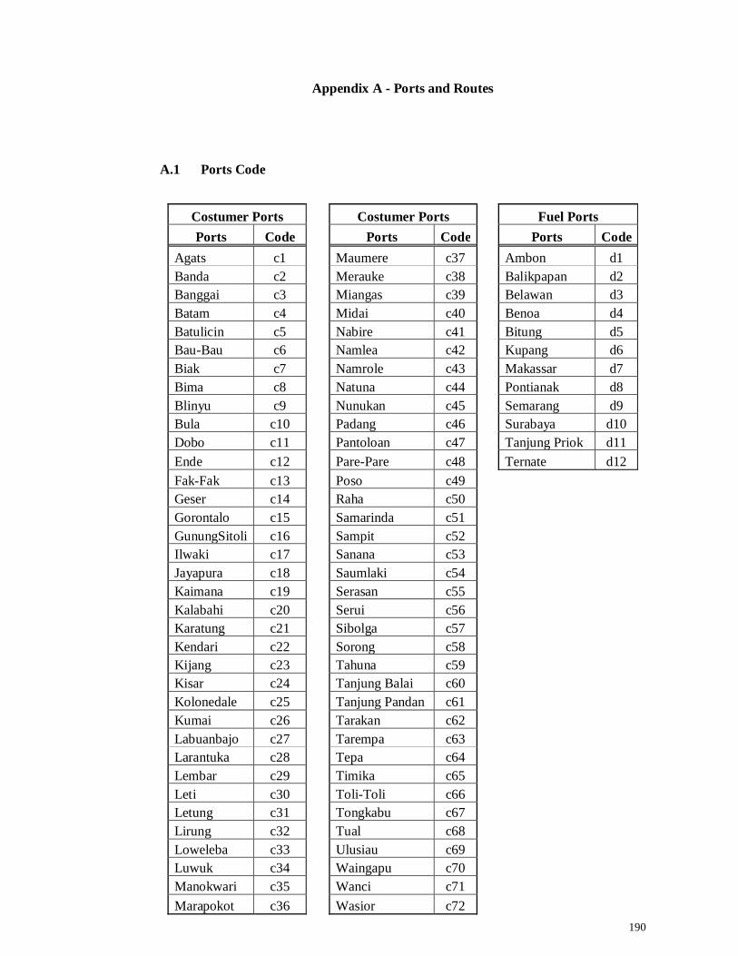
190

Appendix A - Ports and Routes

A.1 Ports Code

Costumer Ports Costumer Ports Fuel Ports Ports Code Ports Code Ports Code

Agats c1 Maumere c37 Ambon d1 Banda c2 Merauke c38 Balikpapan d2 Banggai c3 Miangas c39 Belawan d3 Batam c4 Midai c40 Benoa d4 Batulicin c5 Nabire c41 Bitung d5 Bau-Bau c6 Namlea c42 Kupang d6 Biak c7 Namrole c43 Makassar d7 Bima c8 Natuna c44 Pontianak d8 Blinyu c9 Nunukan c45 Semarang d9 Bula c10 Padang c46 Surabaya d10 Dobo c11 Pantoloan c47 Tanjung Priok d11 Ende c12 Pare-Pare c48 Ternate d12 Fak-Fak c13 Poso c49 Geser c14 Raha c50 Gorontalo c15 Samarinda c51 GunungSitoli c16 Sampit c52 Ilwaki c17 Sanana c53 Jayapura c18 Saumlaki c54 Kaimana c19 Serasan c55 Kalabahi c20 Serui c56 Karatung c21 Sibolga c57 Kendari c22 Sorong c58 Kijang c23 Tahuna c59 Kisar c24 Tanjung Balai c60 Kolonedale c25 Tanjung Pandan c61 Kumai c26 Tarakan c62 Labuanbajo c27 Tarempa c63 Larantuka c28 Tepa c64 Lembar c29 Timika c65 Leti c30 Toli-Toli c66 Letung c31 Tongkabu c67 Lirung c32 Tual c68 Loweleba c33 Ulusiau c69 Luwuk c34 Waingapu c70 Manokwari c35 Wanci c71 Marapokot c36 Wasior c72

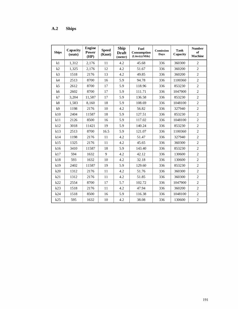
191

A.2 Ships

Ships Capacity (seats)

Engine Power (HP)

Speed (Knot)

Ship Draft (meter)

Fuel Consumption (Liter(s)/Mile)

Comission Days

Tank Capacity

Number of

Machine

k1 1,312 2,176 11 4.2 45.68 336 360300 2 k2 1,325 2,176 12 4.2 51.67 336 360200 2 k3 1518 2176 13 4.2 49.85 336 360200 2 k4 2513 8700 16 5.9 94.78 336 1100360 2 k5 2612 8700 17 5.9 118.96 336 853230 2 k6 2602 8700 17 5.9 111.71 336 1047900 2 k7 3,204 11,587 17 5.9 136.58 336 853230 2 k8 1,583 8,160 18 5.9 108.69 336 1048100 2 k9 1198 2176 10 4.2 56.82 336 327940 2

k10 2404 11587 18 5.9 127.51 336 853230 2 k11 2126 8500 16 5.9 117.02 336 1048100 2 k12 3018 11421 19 5.9 140.24 336 853230 2 k13 2513 8700 16.5 5.9 121.07 336 1100360 2 k14 1198 2176 11 4.2 51.47 336 327940 2 k15 1325 2176 11 4.2 45.65 336 360300 2 k16 3410 11587 18 5.9 143.40 336 853230 2 k17 594 1632 9 4.2 42.12 336 130600 2 k18 593 1632 10 4.2 32.18 336 130600 2 k19 2402 11587 19 5.9 129.60 336 853230 2 k20 1312 2176 11 4.2 51.76 336 360300 2 k21 1312 2176 11 4.2 51.85 336 360300 2 k22 2554 8700 17 5.7 102.72 336 1047900 2 k23 1518 2176 11 4.2 47.94 336 360200 2 k24 1518 8500 16 5.9 116.38 336 1048100 2 k25 595 1632 10 4.2 38.08 336 130600 2

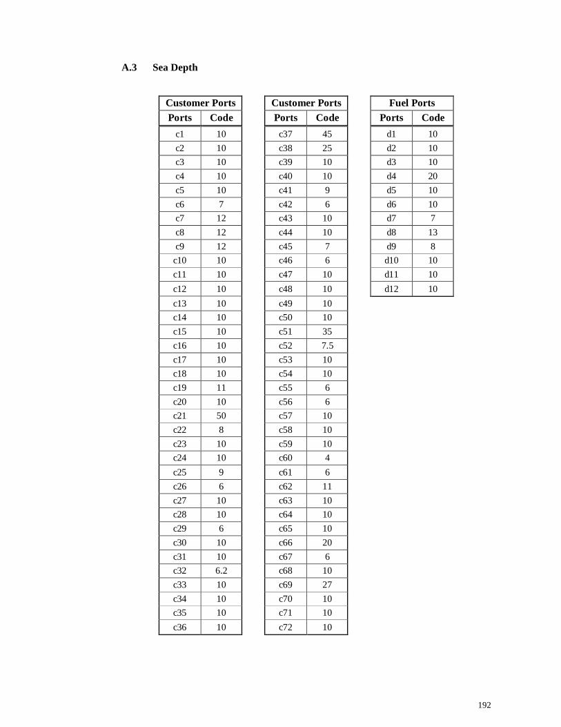
192

A.3 Sea Depth

Customer Ports Customer Ports Fuel Ports Ports Code Ports Code Ports Code

c1 10 c37 45 d1 10 c2 10 c38 25 d2 10 c3 10 c39 10 d3 10 c4 10 c40 10 d4 20 c5 10 c41 9 d5 10 c6 7 c42 6 d6 10 c7 12 c43 10 d7 7 c8 12 c44 10 d8 13 c9 12 c45 7 d9 8

c10 10 c46 6 d10 10 c11 10 c47 10 d11 10 c12 10 c48 10 d12 10 c13 10 c49 10 c14 10 c50 10 c15 10 c51 35 c16 10 c52 7.5 c17 10 c53 10 c18 10 c54 10 c19 11 c55 6 c20 10 c56 6 c21 50 c57 10 c22 8 c58 10 c23 10 c59 10 c24 10 c60 4 c25 9 c61 6 c26 6 c62 11 c27 10 c63 10 c28 10 c64 10 c29 6 c65 10 c30 10 c66 20 c31 10 c67 6 c32 6.2 c68 10 c33 10 c69 27 c34 10 c70 10 c35 10 c71 10 c36 10 c72 10

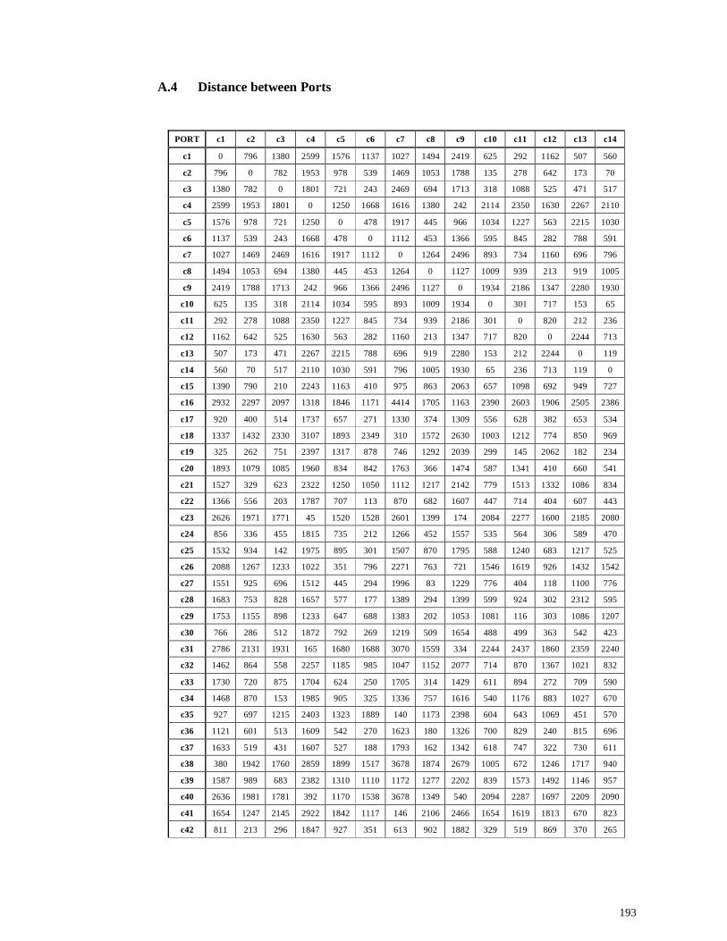
193

A.4 Distance between Ports

PORT c1 c2 c3 c4 c5 c6 c7 c8 c9 c10 c11 c12 c13 c14

c1 0 796 1380 2599 1576 1137 1027 1494 2419 625 292 1162 507 560

c2 796 0 782 1953 978 539 1469 1053 1788 135 278 642 173 70

c3 1380 782 0 1801 721 243 2469 694 1713 318 1088 525 471 517

c4 2599 1953 1801 0 1250 1668 1616 1380 242 2114 2350 1630 2267 2110

c5 1576 978 721 1250 0 478 1917 445 966 1034 1227 563 2215 1030

c6 1137 539 243 1668 478 0 1112 453 1366 595 845 282 788 591

c7 1027 1469 2469 1616 1917 1112 0 1264 2496 893 734 1160 696 796

c8 1494 1053 694 1380 445 453 1264 0 1127 1009 939 213 919 1005

c9 2419 1788 1713 242 966 1366 2496 1127 0 1934 2186 1347 2280 1930

c10 625 135 318 2114 1034 595 893 1009 1934 0 301 717 153 65

c11 292 278 1088 2350 1227 845 734 939 2186 301 0 820 212 236

c12 1162 642 525 1630 563 282 1160 213 1347 717 820 0 2244 713

c13 507 173 471 2267 2215 788 696 919 2280 153 212 2244 0 119

c14 560 70 517 2110 1030 591 796 1005 1930 65 236 713 119 0

c15 1390 790 210 2243 1163 410 975 863 2063 657 1098 692 949 727

c16 2932 2297 2097 1318 1846 1171 4414 1705 1163 2390 2603 1906 2505 2386

c17 920 400 514 1737 657 271 1330 374 1309 556 628 382 653 534

c18 1337 1432 2330 3107 1893 2349 310 1572 2630 1003 1212 774 850 969

c19 325 262 751 2397 1317 878 746 1292 2039 299 145 2062 182 234

c20 1893 1079 1085 1960 834 842 1763 366 1474 587 1341 410 660 541

c21 1527 329 623 2322 1250 1050 1112 1217 2142 779 1513 1332 1086 834

c22 1366 556 203 1787 707 113 870 682 1607 447 714 404 607 443

c23 2626 1971 1771 45 1520 1528 2601 1399 174 2084 2277 1600 2185 2080

c24 856 336 455 1815 735 212 1266 452 1557 535 564 306 589 470

c25 1532 934 142 1975 895 301 1507 870 1795 588 1240 683 1217 525

c26 2088 1267 1233 1022 351 796 2271 763 721 1546 1619 926 1432 1542

c27 1551 925 696 1512 445 294 1996 83 1229 776 404 118 1100 776

c28 1683 753 828 1657 577 177 1389 294 1399 599 924 302 2312 595

c29 1753 1155 898 1233 647 688 1383 202 1053 1081 116 303 1086 1207

c30 766 286 512 1872 792 269 1219 509 1654 488 499 363 542 423

c31 2786 2131 1931 165 1680 1688 3070 1559 334 2244 2437 1860 2359 2240

c32 1462 864 558 2257 1185 985 1047 1152 2077 714 870 1367 1021 832

c33 1730 720 875 1704 624 250 1705 314 1429 611 894 272 709 590

c34 1468 870 153 1985 905 325 1336 757 1616 540 1176 883 1027 670

c35 927 697 1215 2403 1323 1889 140 1173 2398 604 643 1069 451 570

c36 1121 601 513 1609 542 270 1623 180 1326 700 829 240 815 696

c37 1633 519 431 1607 527 188 1793 162 1342 618 747 322 730 611

c38 380 1942 1760 2859 1899 1517 3678 1874 2679 1005 672 1246 1717 940

c39 1587 989 683 2382 1310 1110 1172 1277 2202 839 1573 1492 1146 957

c40 2636 1981 1781 392 1170 1538 3678 1349 540 2094 2287 1697 2209 2090

c41 1654 1247 2145 2922 1842 1117 146 2106 2466 1654 1619 1813 670 823

c42 811 213 296 1847 927 351 613 902 1882 329 519 869 370 265

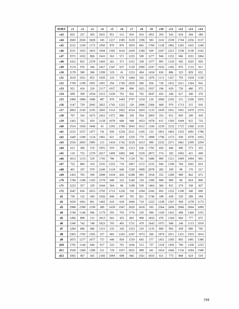
194

PORT c1 c2 c3 c4 c5 c6 c7 c8 c9 c10 c11 c12 c13 c14

c43 835 237 305 2031 951 512 810 916 1851 293 543 634 394 289

c44 2683 2026 1828 345 1217 1585 3218 1396 583 2141 2339 1744 2256 2137

c45 2152 1339 1173 1950 870 876 1819 845 1760 1128 1862 1265 1435 1246

c46 2531 1933 1853 1094 1302 1610 2439 1349 929 2247 2212 1538 2138 2162

c47 1972 1032 866 1643 563 571 1235 508 1277 946 1252 666 1031 1064

c48 1412 832 2378 1443 261 371 1312 338 1377 905 1120 583 1025 920

c49 1574 976 394 2427 1347 637 1159 1090 2247 1032 1282 876 1133 911

c50 1178 580 386 1599 519 41 1153 494 1434 636 886 323 829 632

c51 1619 1021 853 1650 233 578 1444 545 1470 1111 1327 793 1418 1130

c52 1769 1189 1091 1001 294 1769 2029 696 836 728 1451 1611 1364 943

c53 921 416 220 2117 1037 598 896 1021 1937 196 629 720 480 375

c54 608 300 1034 2212 1230 791 832 792 2047 435 240 617 340 370

c55 2484 1886 1686 487 870 1443 3707 1254 120 2060 2192 515 2100 1955

c56 1147 729 2045 2822 1742 1222 120 2006 2366 668 979 1713 515 916

c57 2863 2145 2195 2065 1514 1822 4314 1693 1133 2439 2451 1941 2479 2374

c58 707 316 1675 2452 1372 886 320 954 2003 353 912 850 200 418

c59 1363 765 459 2158 1078 600 948 1053 1978 615 1393 1049 922 733

c60 2524 1926 1846 45 1295 1789 3043 1612 1106 2220 2232 1722 2260 2155

c61 2155 1557 1477 741 926 1234 2511 1105 153 1851 1863 1353 1891 1786

c62 1449 1290 1124 1901 821 829 1259 770 1898 1790 1273 928 1078 1955

c63 2556 2065 1985 215 1434 1742 3218 1613 999 2332 2371 1861 2399 2294

c64 612 306 519 1955 919 396 1313 636 1781 420 446 490 573 355

c65 110 752 1270 2617 1409 1685 848 1559 2873 574 182 1002 421 449

c66 1813 1215 529 1745 786 794 1120 761 1686 989 1521 1009 1094 905

c67 752 884 310 2335 1255 719 1067 1172 2155 940 1190 784 1041 819

c68 401 197 979 2240 1118 640 1330 1009 2078 282 109 98 170 217

c69 1303 705 399 2098 1018 826 6188 993 1918 555 1289 989 862 673

c70 1784 1186 1192 1579 949 552 1240 150 1399 998 900 98 854 890

c71 1223 357 329 1644 564 86 1198 539 1464 366 931 374 530 427

c72 1047 656 2015 2792 1712 1226 150 1294 2343 693 1252 1190 540 690

d1 730 132 200 1926 846 407 705 821 1746 188 438 529 289 184

d2 1659 1061 861 1402 610 618 1694 710 1222 1238 1367 958 1278 1173

d3 2988 2390 2190 389 1639 1947 3020 1818 593 2564 2696 2066 2604 2499

d4 1744 1146 946 1179 595 703 1776 250 999 1320 1452 498 1360 1255

d5 1496 898 212 2013 941 455 803 908 1833 470 1204 904 777 672

d6 1340 742 748 1823 705 405 1731 479 1643 1075 948 146 1115 1010

d7 1284 686 486 1315 235 243 1223 210 1135 860 992 458 900 795

d8 2303 1705 1505 327 682 1262 2247 1073 260 1879 2011 1321 1919 1814

d9 1875 1277 1077 757 446 834 1319 645 577 1451 1583 893 1491 1386

d10 1792 1144 944 917 333 701 1636 512 737 1318 1450 760 1358 1253

d11 1958 1360 1280 521 729 1037 2022 908 341 1654 1666 1156 1694 1589

d12 1065 467 365 2166 1094 608 666 1561 1833 411 773 868 624 519

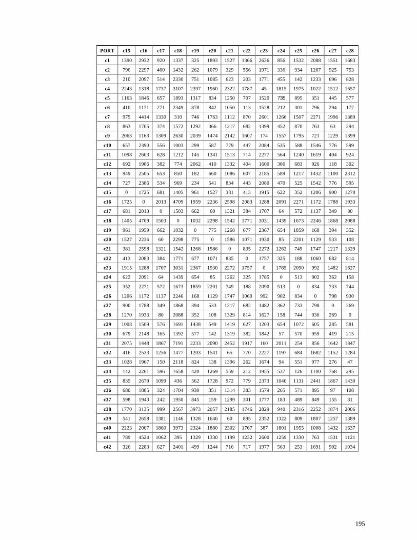
195

PORT c15 c16 c17 c18 c19 c20 c21 c22 c23 c24 c25 c26 c27 c28

c1 1390 2932 920 1337 325 1893 1527 1366 2626 856 1532 2088 1551 1683

c2 790 2297 400 1432 262 1079 329 556 1971 336 934 1267 925 753

c3 210 2097 514 2330 751 1085 623 203 1771 455 142 1233 696 828

c4 2243 1318 1737 3107 2397 1960 2322 1787 45 1815 1975 1022 1512 1657

c5 1163 1846 657 1893 1317 834 1250 707 1520 735 895 351 445 577

c6 410 1171 271 2349 878 842 1050 113 1528 212 301 796 294 177

c7 975 4414 1330 310 746 1763 1112 870 2601 1266 1507 2271 1996 1389

c8 863 1705 374 1572 1292 366 1217 682 1399 452 870 763 63 294

c9 2063 1163 1309 2630 2039 1474 2142 1607 174 1557 1795 721 1229 1399

c10 657 2390 556 1003 299 587 779 447 2084 535 588 1546 776 599

c11 1098 2603 628 1212 145 1341 1513 714 2277 564 1240 1619 404 924

c12 692 1906 382 774 2062 410 1332 404 1600 306 683 926 118 302

c13 949 2505 653 850 182 660 1086 607 2185 589 1217 1432 1100 2312

c14 727 2386 534 969 234 541 834 443 2080 470 525 1542 776 595

c15 0 1725 681 1405 961 1527 381 413 1915 622 352 1206 900 1270

c16 1725 0 2013 4709 1959 2236 2598 2083 1288 2091 2271 1172 1788 1933

c17 681 2013 0 1503 662 60 1321 384 1707 64 572 1137 349 80

c18 1405 4709 1503 0 1032 2298 1542 1771 3031 1439 1673 2246 1868 2088

c19 961 1959 662 1032 0 775 1268 677 2367 654 1859 168 394 352

c20 1527 2236 60 2298 775 0 1586 1071 1930 85 2201 1129 533 108

c21 381 2598 1321 1542 1268 1586 0 835 2272 1262 749 1747 1217 1329

c22 413 2083 384 1771 677 1071 835 0 1757 325 188 1060 682 814

c23 1915 1288 1707 3031 2367 1930 2272 1757 0 1785 2090 992 1482 1627

c24 622 2091 64 1439 654 85 1262 325 1785 0 513 902 362 158

c25 352 2271 572 1673 1859 2201 749 188 2090 513 0 834 733 744

c26 1206 1172 1137 2246 168 1129 1747 1060 992 902 834 0 798 930

c27 900 1788 349 1868 394 533 1217 682 1482 362 733 798 0 269

c28 1270 1933 80 2088 352 108 1329 814 1627 158 744 930 269 0

c29 1008 1509 576 1691 1438 549 1419 627 1203 654 1072 605 285 581

c30 679 2148 165 1392 577 142 1319 382 1842 57 570 959 419 215

c31 2075 1448 1867 7191 2233 2090 2452 1917 160 2011 254 856 1642 1847

c32 416 2533 1256 1477 1203 1541 65 770 2227 1197 684 1682 1152 1284

c33 1028 1967 150 2118 824 138 1396 262 1674 94 551 977 276 47

c34 142 2261 596 1658 420 1269 559 212 1955 537 126 1100 768 295

c35 835 2679 1099 436 562 1728 972 779 2373 1040 1131 2441 1867 1430

c36 680 1885 324 1704 930 351 1314 383 1579 265 571 895 97 108

c37 598 1943 242 1950 845 159 1299 301 1777 183 489 849 155 81

c38 1770 3135 999 2567 3973 2057 2185 1746 2829 940 2316 2252 1874 2006

c39 541 2658 1381 1146 1328 1646 60 895 2352 1322 809 1807 1257 1389

c40 2223 2007 1860 3973 2324 1880 2302 1767 387 1801 1955 1008 1432 1637

c41 789 4524 1062 395 1329 1330 1199 1232 2600 1259 1330 763 1531 1121

c42 326 2283 627 2401 499 1244 716 717 1977 563 253 1691 902 1034

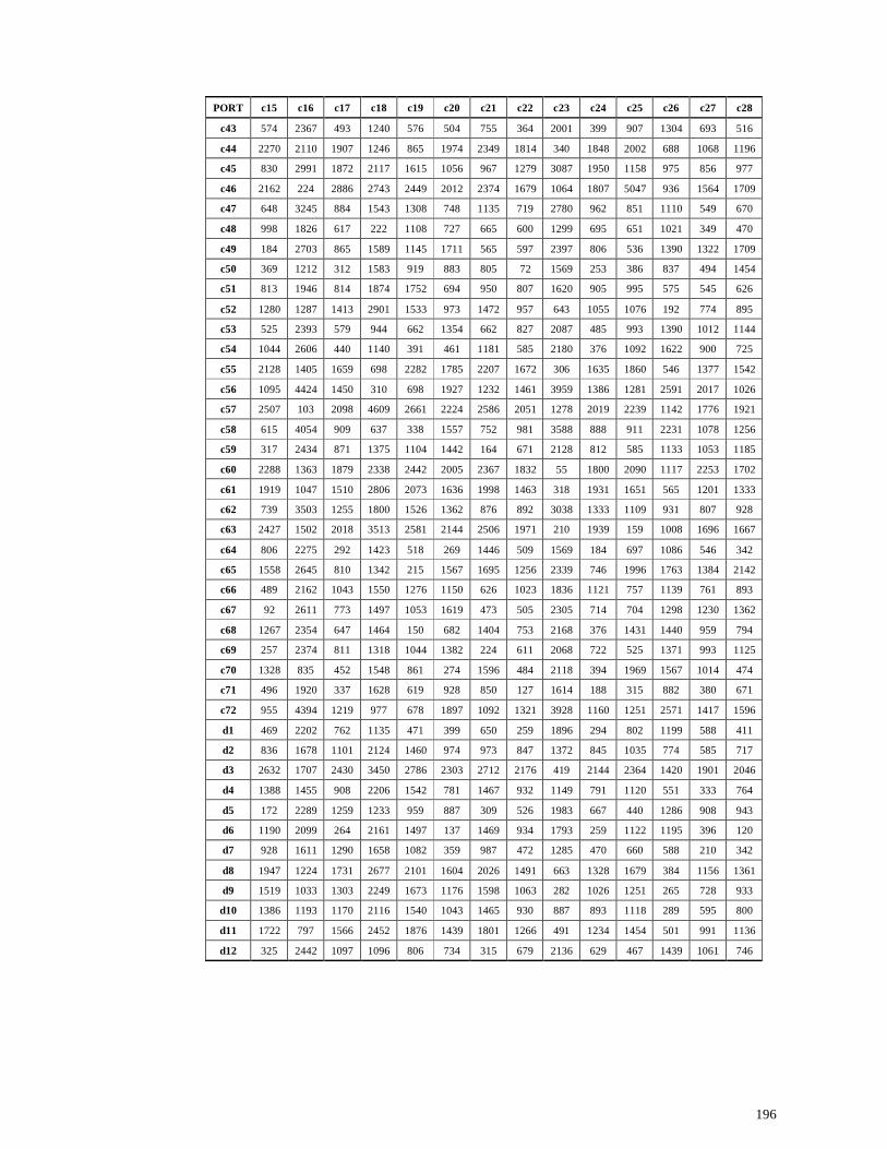
196

PORT c15 c16 c17 c18 c19 c20 c21 c22 c23 c24 c25 c26 c27 c28

c43 574 2367 493 1240 576 504 755 364 2001 399 907 1304 693 516

c44 2270 2110 1907 1246 865 1974 2349 1814 340 1848 2002 688 1068 1196

c45 830 2991 1872 2117 1615 1056 967 1279 3087 1950 1158 975 856 977

c46 2162 224 2886 2743 2449 2012 2374 1679 1064 1807 5047 936 1564 1709

c47 648 3245 884 1543 1308 748 1135 719 2780 962 851 1110 549 670

c48 998 1826 617 222 1108 727 665 600 1299 695 651 1021 349 470

c49 184 2703 865 1589 1145 1711 565 597 2397 806 536 1390 1322 1709

c50 369 1212 312 1583 919 883 805 72 1569 253 386 837 494 1454

c51 813 1946 814 1874 1752 694 950 807 1620 905 995 575 545 626

c52 1280 1287 1413 2901 1533 973 1472 957 643 1055 1076 192 774 895

c53 525 2393 579 944 662 1354 662 827 2087 485 993 1390 1012 1144

c54 1044 2606 440 1140 391 461 1181 585 2180 376 1092 1622 900 725

c55 2128 1405 1659 698 2282 1785 2207 1672 306 1635 1860 546 1377 1542

c56 1095 4424 1450 310 698 1927 1232 1461 3959 1386 1281 2591 2017 1026

c57 2507 103 2098 4609 2661 2224 2586 2051 1278 2019 2239 1142 1776 1921

c58 615 4054 909 637 338 1557 752 981 3588 888 911 2231 1078 1256

c59 317 2434 871 1375 1104 1442 164 671 2128 812 585 1133 1053 1185

c60 2288 1363 1879 2338 2442 2005 2367 1832 55 1800 2090 1117 2253 1702

c61 1919 1047 1510 2806 2073 1636 1998 1463 318 1931 1651 565 1201 1333

c62 739 3503 1255 1800 1526 1362 876 892 3038 1333 1109 931 807 928

c63 2427 1502 2018 3513 2581 2144 2506 1971 210 1939 159 1008 1696 1667

c64 806 2275 292 1423 518 269 1446 509 1569 184 697 1086 546 342

c65 1558 2645 810 1342 215 1567 1695 1256 2339 746 1996 1763 1384 2142

c66 489 2162 1043 1550 1276 1150 626 1023 1836 1121 757 1139 761 893

c67 92 2611 773 1497 1053 1619 473 505 2305 714 704 1298 1230 1362

c68 1267 2354 647 1464 150 682 1404 753 2168 376 1431 1440 959 794

c69 257 2374 811 1318 1044 1382 224 611 2068 722 525 1371 993 1125

c70 1328 835 452 1548 861 274 1596 484 2118 394 1969 1567 1014 474

c71 496 1920 337 1628 619 928 850 127 1614 188 315 882 380 671

c72 955 4394 1219 977 678 1897 1092 1321 3928 1160 1251 2571 1417 1596

d1 469 2202 762 1135 471 399 650 259 1896 294 802 1199 588 411

d2 836 1678 1101 2124 1460 974 973 847 1372 845 1035 774 585 717

d3 2632 1707 2430 3450 2786 2303 2712 2176 419 2144 2364 1420 1901 2046

d4 1388 1455 908 2206 1542 781 1467 932 1149 791 1120 551 333 764

d5 172 2289 1259 1233 959 887 309 526 1983 667 440 1286 908 943

d6 1190 2099 264 2161 1497 137 1469 934 1793 259 1122 1195 396 120

d7 928 1611 1290 1658 1082 359 987 472 1285 470 660 588 210 342

d8 1947 1224 1731 2677 2101 1604 2026 1491 663 1328 1679 384 1156 1361

d9 1519 1033 1303 2249 1673 1176 1598 1063 282 1026 1251 265 728 933

d10 1386 1193 1170 2116 1540 1043 1465 930 887 893 1118 289 595 800

d11 1722 797 1566 2452 1876 1439 1801 1266 491 1234 1454 501 991 1136

d12 325 2442 1097 1096 806 734 315 679 2136 629 467 1439 1061 746

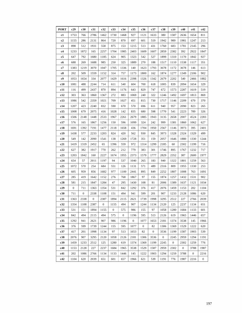
197

PORT c29 c30 c31 c32 c33 c34 c35 c36 c37 c38 c39 c40 c41 c42

c1 1753 766 2786 1462 1730 1468 927 1121 1633 380 1587 2636 1654 811

c2 1155 286 2131 864 720 870 697 601 519 1942 989 1981 1247 213

c3 898 512 1931 558 875 153 1215 513 431 1760 683 1781 2145 296

c4 1233 1872 165 2257 1704 1985 2403 1609 1607 2859 2382 392 2922 1847

c5 647 792 1680 1185 624 905 1323 542 527 1899 1310 1170 1842 927

c6 688 269 1688 985 250 325 1889 270 188 1517 1110 1538 1117 351

c7 1383 1219 3070 1047 1705 1336 140 1623 1793 3678 1172 3678 146 613

c8 202 509 1559 1152 314 757 1173 1800 162 1874 1277 1349 2106 902

c9 1053 1654 334 2077 1429 1616 2398 1326 1342 2679 2202 540 2466 1882

c10 1081 488 2244 714 611 540 604 700 618 1005 839 2094 1654 329

c11 116 499 2437 870 894 1176 643 829 747 672 1573 2287 1619 519

c12 303 363 1860 1367 272 883 1069 240 322 1246 1492 1697 1813 869

c13 1086 542 2359 1021 709 1027 451 815 730 1717 1146 2209 670 370

c14 1207 423 2240 832 590 670 570 696 611 940 957 2090 823 265

c15 1008 679 2075 416 1028 142 835 680 598 1770 541 2223 789 326

c16 1506 2148 1448 2533 1967 2261 2679 1885 1943 3135 2658 2007 4524 2283

c17 576 165 1867 1256 150 596 1099 324 242 999 1381 1860 1062 627

c18 1691 1392 7191 1477 2118 1658 436 1704 1950 2567 1146 3973 395 2401

c19 1438 577 2233 1203 824 420 562 930 845 3973 1328 2324 1329 499

c20 549 142 2090 1541 138 1269 1728 351 159 2057 1646 1880 1330 1244

c21 1419 1319 2452 65 1396 559 972 1314 1299 2185 60 2302 1199 716

c22 627 382 1917 770 262 212 779 383 301 1746 895 1767 1232 717

c23 1203 1842 160 2227 1674 1955 2373 1579 1777 2829 2352 387 2600 1977

c24 654 57 2011 1197 94 537 1040 265 183 940 1322 1801 1259 563

c25 1072 570 254 684 551 126 1131 571 489 2316 809 1955 1330 253

c26 605 959 856 1682 977 1100 2441 895 849 2252 1807 1008 763 1691

c27 285 419 1642 1152 276 768 1867 97 155 1874 1257 1432 1531 902

c28 581 215 1847 1284 47 295 1430 108 81 2006 1389 1637 1121 1034

c29 0 711 1363 1354 531 842 1292 376 417 2076 1459 1153 202 1104

c30 711 0 2338 1108 151 494 941 599 201 907 1233 2128 1086 620

c31 1363 2338 0 2387 1894 2115 2621 1739 1998 3295 2512 227 2766 2039

c32 1354 1108 2387 0 1155 494 907 1244 1134 2120 125 2237 1134 651

c33 531 151 1894 1155 0 575 986 155 97 1058 1280 1684 1133 601

c34 842 494 2115 494 575 0 1196 595 513 2126 619 1965 1446 657

c35 1292 941 2621 907 986 1196 0 1077 1653 2181 1374 3538 145 1966

c36 376 599 1739 1244 155 595 1077 0 82 1306 1369 1529 1222 620

c37 417 201 1998 1134 97 513 1653 82 0 3536 1199 1587 1903 539

c38 2076 907 3295 2120 1058 2126 2181 1306 3536 0 2245 2959 1294 1191

c39 1459 1233 2512 125 1280 619 1374 1369 1199 2245 0 2302 1259 776

c40 1153 2128 227 2237 1684 1965 3538 1529 1587 2959 2302 0 3788 1987

c41 202 1086 2766 1134 1133 1446 145 1222 1903 1294 1259 3788 0 2216

c42 1104 620 2039 651 601 657 1966 621 539 1191 776 1987 2216 0

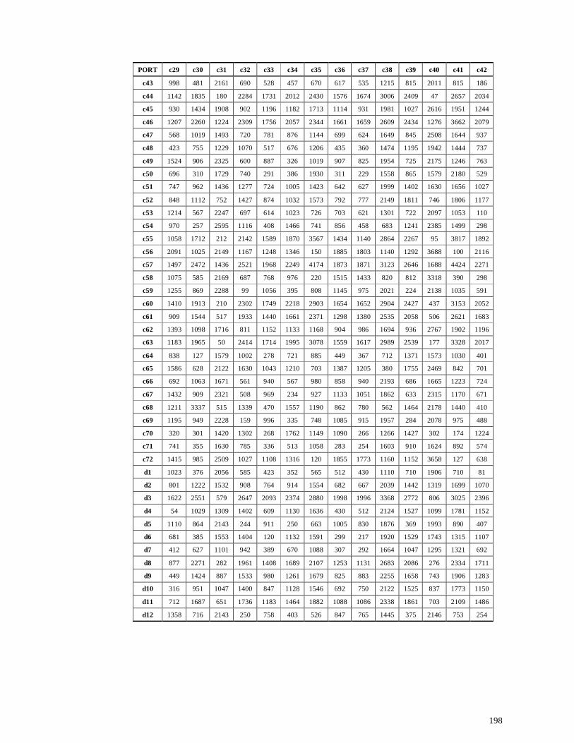
198

PORT c29 c30 c31 c32 c33 c34 c35 c36 c37 c38 c39 c40 c41 c42

c43 998 481 2161 690 528 457 670 617 535 1215 815 2011 815 186

c44 1142 1835 180 2284 1731 2012 2430 1576 1674 3006 2409 47 2657 2034

c45 930 1434 1908 902 1196 1182 1713 1114 931 1981 1027 2616 1951 1244

c46 1207 2260 1224 2309 1756 2057 2344 1661 1659 2609 2434 1276 3662 2079

c47 568 1019 1493 720 781 876 1144 699 624 1649 845 2508 1644 937

c48 423 755 1229 1070 517 676 1206 435 360 1474 1195 1942 1444 737

c49 1524 906 2325 600 887 326 1019 907 825 1954 725 2175 1246 763

c50 696 310 1729 740 291 386 1930 311 229 1558 865 1579 2180 529

c51 747 962 1436 1277 724 1005 1423 642 627 1999 1402 1630 1656 1027

c52 848 1112 752 1427 874 1032 1573 792 777 2149 1811 746 1806 1177

c53 1214 567 2247 697 614 1023 726 703 621 1301 722 2097 1053 110

c54 970 257 2595 1116 408 1466 741 856 458 683 1241 2385 1499 298

c55 1058 1712 212 2142 1589 1870 3567 1434 1140 2864 2267 95 3817 1892

c56 2091 1025 2149 1167 1248 1346 150 1885 1803 1140 1292 3688 100 2116

c57 1497 2472 1436 2521 1968 2249 4174 1873 1871 3123 2646 1688 4424 2271

c58 1075 585 2169 687 768 976 220 1515 1433 820 812 3318 390 298

c59 1255 869 2288 99 1056 395 808 1145 975 2021 224 2138 1035 591

c60 1410 1913 210 2302 1749 2218 2903 1654 1652 2904 2427 437 3153 2052

c61 909 1544 517 1933 1440 1661 2371 1298 1380 2535 2058 506 2621 1683

c62 1393 1098 1716 811 1152 1133 1168 904 986 1694 936 2767 1902 1196

c63 1183 1965 50 2414 1714 1995 3078 1559 1617 2989 2539 177 3328 2017

c64 838 127 1579 1002 278 721 885 449 367 712 1371 1573 1030 401

c65 1586 628 2122 1630 1043 1210 703 1387 1205 380 1755 2469 842 701

c66 692 1063 1671 561 940 567 980 858 940 2193 686 1665 1223 724

c67 1432 909 2321 508 969 234 927 1133 1051 1862 633 2315 1170 671

c68 1211 3337 515 1339 470 1557 1190 862 780 562 1464 2178 1440 410

c69 1195 949 2228 159 996 335 748 1085 915 1957 284 2078 975 488

c70 320 301 1420 1302 268 1762 1149 1090 266 1266 1427 302 174 1224

c71 741 355 1630 785 336 513 1058 283 254 1603 910 1624 892 574

c72 1415 985 2509 1027 1108 1316 120 1855 1773 1160 1152 3658 127 638

d1 1023 376 2056 585 423 352 565 512 430 1110 710 1906 710 81

d2 801 1222 1532 908 764 914 1554 682 667 2039 1442 1319 1699 1070

d3 1622 2551 579 2647 2093 2374 2880 1998 1996 3368 2772 806 3025 2396

d4 54 1029 1309 1402 609 1130 1636 430 512 2124 1527 1099 1781 1152

d5 1110 864 2143 244 911 250 663 1005 830 1876 369 1993 890 407

d6 681 385 1553 1404 120 1132 1591 299 217 1920 1529 1743 1315 1107

d7 412 627 1101 942 389 670 1088 307 292 1664 1047 1295 1321 692

d8 877 2271 282 1961 1408 1689 2107 1253 1131 2683 2086 276 2334 1711

d9 449 1424 887 1533 980 1261 1679 825 883 2255 1658 743 1906 1283

d10 316 951 1047 1400 847 1128 1546 692 750 2122 1525 837 1773 1150

d11 712 1687 651 1736 1183 1464 1882 1088 1086 2338 1861 703 2109 1486

d12 1358 716 2143 250 758 403 526 847 765 1445 375 2146 753 254

199

PORT c43 c44 c45 c46 c47 c48 c49 c50 c51 c52 c53 c54 c55 c56

c1 835 2683 2152 2531 1972 1412 1574 1178 1619 1769 921 608 2484 1147

c2 237 2026 1339 1933 1032 832 976 580 1021 1189 416 300 1886 729

c3 305 1828 1173 1853 866 2378 394 386 853 1091 220 1034 1686 2045

c4 2031 345 1950 1094 1643 1443 2427 1599 1650 1001 2117 2212 487 2822

c5 951 1217 870 1302 563 261 1347 519 233 294 1037 1130 870 1742

c6 512 1585 876 1610 571 371 637 41 578 1769 598 791 1443 1222

c7 810 3218 1819 2439 1235 1312 1159 1153 1444 2029 896 832 3707 120

c8 916 1396 845 1349 508 338 1090 494 545 696 1021 792 1254 2006

c9 1851 583 1760 929 1277 1377 2247 1434 1470 836 1937 2047 120 2366

c10 293 2141 1128 2247 946 905 1032 636 1111 728 196 435 2060 668

c11 543 2339 1862 2212 1252 1120 1282 886 1327 1451 629 240 2192 979

c12 634 1744 1265 1538 666 583 876 323 793 1611 720 617 515 1713

c13 394 2256 1435 2138 1031 1025 1133 829 1418 1364 480 340 2100 515

c14 289 2137 1246 2162 1064 920 911 623 1130 943 375 370 1955 916

c15 574 2270 830 2162 648 998 184 369 813 1280 525 1044 2128 1095

c16 2367 210 2991 224 3245 1826 2703 1212 1946 1287 2393 2606 1405 4424

c17 493 1907 1872 2886 884 617 865 312 814 1413 579 440 1659 1450

c18 1240 1246 2117 2743 1543 222 1589 1583 1874 2901 944 1140 698 310

c19 576 865 1615 2449 1308 1108 1945 919 1752 1533 662 391 2282 698

c20 504 1974 1056 2012 748 727 1711 883 694 973 1354 461 1785 1927

c21 755 2349 967 2374 1135 665 565 805 950 1472 662 1181 2207 1232

c22 364 1814 1279 1679 719 600 597 72 807 957 827 585 1672 1461

c23 2001 340 3087 1064 2780 1299 2397 1569 1620 643 2087 2180 306 3959

c24 399 1848 1950 1807 962 695 806 253 905 1055 485 376 1635 1386

c25 907 2002 1158 5047 851 651 536 386 995 1076 993 1092 1860 1281

c26 1304 688 975 936 1110 1021 1390 837 575 192 1390 1622 546 2591

c27 693 1068 856 1564 549 349 1322 494 545 774 1012 900 1377 2017

c28 516 1196 977 1709 670 470 1709 1454 626 895 1144 725 1542 1026

c29 998 1142 930 1207 568 423 1524 696 747 848 1214 970 1058 2091

c30 481 1835 1434 2260 1019 755 906 310 962 1112 567 257 1712 1025

c31 2161 180 1908 1224 1493 1229 2325 1729 1436 752 2247 2595 212 2149

c32 690 2284 902 2309 720 1070 600 740 1277 1427 697 1116 2142 1167

c33 528 1731 1196 1756 781 517 887 291 724 874 614 408 1589 1248

c34 457 2012 1182 2057 876 676 326 386 1005 1032 1023 1466 1870 1346

c35 670 2430 1713 2344 1144 1206 1019 1930 1423 1573 726 741 3567 150

c36 617 1576 1114 1661 699 435 907 311 642 792 703 856 1434 1885

c37 535 1674 931 1659 624 360 825 229 627 777 621 458 1140 1803

c38 1215 3006 1981 2609 1649 1474 1954 1558 1999 2149 1301 683 2864 1140

c39 815 2409 1027 2434 845 1195 725 865 1402 1811 722 1241 2267 1292

c40 2011 47 2616 1276 2508 1942 2175 1579 1630 746 2097 2385 95 3688

c41 815 2657 1951 3662 1644 1444 1246 2180 1656 1806 1053 1499 3817 100

c42 186 2034 1244 2079 937 737 763 529 1027 1127 110 298 1892 2116

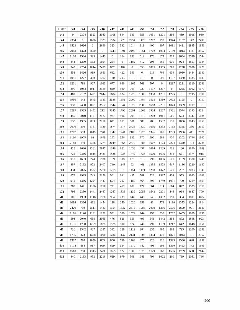
200

PORT c43 c44 c45 c46 c47 c48 c49 c50 c51 c52 c53 c54 c55 c56

c43 0 2394 1523 2083 1108 844 949 553 1051 1201 296 489 1916 930

c44 2394 0 1626 1323 1534 1270 2254 1426 1277 793 1944 2137 142 2490

c45 1523 1626 0 2690 323 532 1014 919 400 907 1011 1431 2845 1851

c46 2083 1323 2690 0 1443 1594 2499 1651 1702 1063 2189 2044 1181 3562

c47 1108 1534 323 1443 0 264 832 612 170 677 829 1684 2536 1544

c48 844 1270 532 1594 264 0 1182 412 293 666 930 924 1851 1344

c49 949 2254 1014 2499 832 1182 0 553 1815 1365 709 1228 2000 1279

c50 553 1426 919 1651 612 412 553 0 619 769 639 1080 1484 2080

c51 1051 1277 400 1702 170 293 1815 619 0 507 1137 1330 1535 1683

c52 1201 793 907 1063 677 666 1365 769 507 0 1287 1281 1310 2281

c53 296 1944 1011 2189 829 930 709 639 1137 1287 0 1225 2002 1073

c54 489 2137 1431 2044 1684 924 1228 1080 1330 1281 1225 0 2195 1309

c55 1916 142 2845 1181 2536 1851 2000 1484 1535 1310 2002 2195 0 3717

c56 930 2490 1851 3562 1544 1344 1279 2080 1683 2281 1073 1309 3717 0

c57 2295 1535 3452 212 3145 1798 2691 1863 1914 1267 2381 2574 1393 4324

c58 450 2010 1101 2127 927 996 799 1710 1203 1911 506 624 3347 360

c59 738 1985 803 2210 621 971 501 680 786 1587 537 1056 2043 1068

c60 2076 390 2181 1139 1874 1674 2426 1830 1695 1232 2162 2355 336 3053

c61 1707 553 1649 770 1342 1241 2103 1275 1326 700 1793 1986 411 2521

c62 1160 1905 91 1699 292 556 923 870 290 883 920 1202 2796 1802

c63 2188 130 2356 1274 2049 1664 2379 1783 1607 1123 2274 2320 194 3228

c64 425 1620 1561 2847 1146 882 1033 437 1084 1239 511 130 1820 1109

c65 725 2316 1815 2421 1528 1228 1742 1736 1509 1696 811 671 2374 918

c66 910 1693 274 1938 159 398 673 813 290 1036 670 1189 1570 1240

c67 857 2162 922 2407 740 1148 92 461 1355 1505 617 1136 2220 1187

c68 434 2025 1522 2270 1215 1016 1451 1171 1218 1372 520 207 2083 1340

c69 678 1925 743 2150 561 911 437 581 726 1527 434 953 1983 1008

c70 915 1366 1224 1447 604 797 1189 865 695 1759 1001 709 1769 1869

c71 287 1471 1136 1716 721 457 680 127 664 814 684 877 1529 1318

c72 796 2350 1441 2467 1267 1336 1139 2056 1543 2201 846 964 3687 700

d1 105 1953 1146 1978 964 739 844 448 946 1362 191 384 1811 825

d2 1094 1366 432 1454 188 250 1020 659 43 778 1180 1373 1224 1814

d3 2420 759 2511 1483 1154 1832 2816 1988 2039 1236 2506 2699 901 3140

d4 1176 1146 1181 1231 931 588 1572 744 795 555 1262 1455 1009 1896

d5 593 2040 658 2065 476 826 356 496 641 1442 353 872 1898 923

d6 1131 1790 1269 1875 1575 590 574 746 797 1199 1217 642 1648 1851

d7 716 1342 807 1387 392 128 1112 284 335 485 802 795 1200 1348

d8 1735 323 1478 1000 1234 1147 2131 1303 1354 470 1821 2014 181 2367

d9 1307 790 1050 809 806 719 1703 875 926 326 1393 1586 648 1939

d10 1174 884 917 969 669 514 1570 742 793 293 1260 1453 742 1806

d11 1510 750 1313 573 1065 922 1906 1078 1129 562 1596 1789 608 2142

d12 440 2193 952 2218 629 979 509 649 794 1602 200 719 2051 786

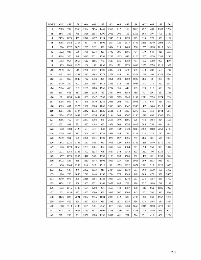
201

PORT c57 c58 c59 c60 c61 c62 c63 c64 c65 c66 c67 c68 c69 c70

c1 2863 707 1363 2524 2155 1449 2556 612 110 1813 752 401 1303 1784

c2 2145 316 765 1926 1557 1290 2065 306 752 1215 884 197 705 1186

c3 2195 1675 459 2846 1477 1124 1945 519 1270 529 310 979 399 1192

c4 2065 2452 2158 45 741 1901 215 1955 2617 1745 2335 2240 2098 1579

c5 1514 1372 1078 1295 926 821 1434 919 1409 786 1255 1118 1018 949

c6 1822 886 600 1789 1234 829 1742 396 1685 794 719 640 826 552

c7 4314 320 948 3043 2511 1259 3218 1313 848 1120 1067 1330 6188 1240

c8 1693 954 1053 1612 1105 770 1613 636 1559 761 1172 1009 993 150

c9 1133 2003 1978 1106 153 1898 999 1781 2873 1686 2155 2078 1918 1399

c10 2439 353 615 2220 1851 1790 2332 420 574 989 940 282 555 998

c11 2451 912 1393 2232 1863 1273 2371 446 182 1521 1190 109 1289 900

c12 1941 850 1049 1722 1353 928 1861 490 1002 1009 784 98 989 98

c13 2479 200 922 2260 1891 1078 2399 573 421 1094 1041 170 862 854

c14 2374 418 733 2155 1786 1955 2294 355 449 905 819 217 673 890

c15 2507 615 317 2288 1919 739 2427 806 1558 489 92 1267 257 1328

c16 80 4054 2434 1363 1047 3503 1502 2275 2645 2162 2611 2354 2374 835

c17 2098 909 871 1879 1510 1255 2018 292 810 1043 773 647 811 452

c18 4609 637 1375 2338 2806 1800 3513 1423 1342 1550 1497 1464 1318 1548

c19 2661 338 1104 2442 2073 1526 2581 518 215 1276 1053 150 1044 861

c20 2224 1557 1442 2005 1636 1362 2144 269 1567 1150 1619 682 1382 274

c21 2586 752 164 2367 1998 876 2506 1446 1695 626 473 1404 224 1596

c22 2051 981 671 1832 1463 892 1971 509 1256 1023 505 753 611 484

c23 1278 3588 2128 55 318 3038 210 1569 2339 1836 2305 2168 2068 2118

c24 2019 888 812 1800 1931 1333 1939 184 746 1121 714 376 722 394

c25 2239 911 585 2090 1651 1109 159 697 1996 757 704 1431 525 1969

c26 1142 2231 1133 1117 565 931 1008 1086 1763 1139 1298 1440 1371 1567

c27 1776 1078 1053 2253 1201 807 1696 546 1384 761 1230 959 993 1014

c28 1921 1256 1185 1702 1333 928 1667 342 2142 893 1362 794 1125 474

c29 1497 1075 1255 1410 909 1393 1183 838 1586 692 1432 1211 1195 320

c30 2472 585 869 1913 1544 1098 1965 127 628 1063 909 3337 949 301

c31 1436 2169 2288 210 517 1716 50 1579 2122 1671 2321 515 2228 1420

c32 2521 687 99 2302 1933 811 2414 1002 1630 561 508 1339 159 1302

c33 1968 768 1056 1749 1440 1152 1714 278 1043 940 969 470 996 2683

c34 2249 976 395 2218 1661 1133 1995 721 1210 567 234 1557 335 1762

c35 4174 220 808 2903 2371 1168 3078 885 703 980 927 1190 748 1149

c36 1873 1515 1145 1654 1298 904 1559 449 1387 858 1113 862 1085 1090

c37 1871 1433 975 1652 1380 986 1617 367 1205 945 1051 780 915 266

c38 3123 820 2021 2904 2535 1694 2989 712 380 2193 1862 562 1957 1266

c39 2646 812 224 2427 2058 936 2539 1371 1755 686 633 1464 284 1427

c40 1688 3318 2138 437 506 2767 177 1573 2469 1665 2315 2178 2078 302

c41 4424 390 1035 3153 2621 1902 3328 1030 842 1223 1170 1440 975 174

c42 2271 298 591 2052 1683 1196 2017 401 701 724 671 410 488 1224

202

PORT c57 c58 c59 c60 c61 c62 c63 c64 c65 c66 c67 c68 c69 c70

c43 2295 450 738 2076 1707 1160 2188 425 725 910 857 434 678 911

c44 1535 2010 1985 390 553 1905 130 1620 2316 1693 2162 2025 1925 1366

c45 3452 1101 803 2181 1649 90 2356 1561 1815 274 922 1522 743 1224

c46 212 2127 2210 1179 770 1699 1274 2847 2421 1938 2407 2270 2150 1447

c47 3145 927 621 1874 1342 292 2049 1146 1528 159 740 1215 561 604

c48 1798 996 971 1674 1241 556 1664 882 1228 398 1148 1016 911 797

c49 2691 799 501 2426 2103 923 2379 1033 1742 673 92 1451 437 1189

c50 1863 1710 680 1830 1275 870 1783 437 1736 813 461 1171 581 865

c51 1914 1203 786 1695 1326 290 1607 1084 1509 290 1355 1218 726 695

c52 1267 1911 1587 1232 700 883 1123 1239 1696 1036 1505 1372 1527 1759

c53 2381 506 537 2162 1793 920 2274 511 811 670 617 520 434 1001

c54 2574 624 1056 2355 1986 1202 2320 130 671 1189 1136 207 953 709

c55 1393 3347 2043 336 411 2796 194 1820 2374 1570 2220 2083 1983 1769

c56 4324 360 1068 3053 2521 1802 3228 1109 918 1240 1187 1340 1008 1869

c57 0 3954 2090 1355 986 3403 1490 2263 2637 2013 2603 2346 2366 1619

c58 3954 0 588 2683 2151 951 2603 686 594 760 707 334 528 930

c59 2090 588 0 2203 1834 712 2315 996 1253 462 409 1240 60 1203

c60 1355 2683 2203 0 972 2132 420 2185 2848 1790 2380 2471 2143 696

c61 986 2151 1834 972 0 1600 688 1630 2045 1421 2011 1754 1774 690

c62 3403 951 712 2132 1600 0 2307 1225 1675 250 831 1473 652 866

c63 1490 2603 2315 420 688 2307 0 2138 2703 1823 2292 540 2055 640

c64 2263 686 996 2185 1630 1225 2138 0 628 1190 1115 337 1222 578

c65 2637 594 1253 2848 2045 1675 2703 628 0 1703 1372 1719 1193 512

c66 2013 760 462 1790 1421 250 1823 1190 1703 0 581 1412 402 614

c67 2603 707 409 2380 2011 831 2292 1115 1372 581 0 1359 349 1380

c68 2346 334 1240 2471 1754 1473 540 337 1719 1412 1359 0 1180 1255

c69 2366 528 60 2143 1774 652 2055 1222 1193 402 349 1180 0 1143

c70 1619 930 1203 696 690 866 640 578 512 614 1380 1255 1143 0

c71 1912 838 686 1875 1320 915 1828 482 1113 858 588 529 626 638

c72 4294 340 928 3023 2491 1291 2943 1026 934 1100 1047 674 868 1270

d1 2190 345 633 1971 1602 1055 1636 320 620 805 752 329 573 810

d2 1666 1243 809 1447 1078 388 1352 1349 1549 347 928 1258 749 860

d3 1695 2572 2548 344 1130 2467 604 2678 2878 2134 2729 2587 2488 1968

d4 1443 1328 1303 1224 855 1459 1129 1156 1634 1011 1480 1343 1243 400

d5 2277 443 145 2058 1689 567 2023 1002 1386 317 264 1095 85 1058

d6 2087 1330 1305 1868 1499 1225 1773 512 1430 1013 1482 1139 1245 244

d7 1579 868 843 1360 991 763 1125 754 1174 551 1020 883 783 360

d8 1212 1887 1862 738 230 1434 306 1297 2192 1389 2039 1902 1002 1223

d9 1021 1459 1434 802 433 1006 773 1551 1765 961 1611 1474 1374 795

d10 1181 1326 1301 962 593 873 867 1078 1632 828 1478 1341 1241 662

d11 785 1662 1637 566 197 1269 701 1474 1848 1224 1814 1557 1577 1058

d12 2430 306 298 2211 1842 1205 2176 849 955 470 417 664 238 1145

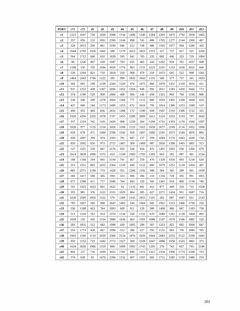
203

PORT c71 c72 d1 d2 d3 d4 d5 d6 d7 d8 d9 d10 d11 d12

c1 1223 1047 730 1659 2988 1744 1496 1340 1284 2303 1875 1792 1958 1065

c2 357 656 132 1061 2390 1146 898 742 686 1705 1277 1144 1360 467

c3 329 2015 200 861 2190 946 212 748 486 1505 1077 944 1280 365

c4 1644 2792 1926 1402 389 1179 2013 1823 1315 327 757 917 521 2166

c5 564 1712 846 610 1639 595 941 705 235 682 446 333 729 1094

c6 86 1226 407 618 1947 703 455 405 243 1262 834 701 1037 608

c7 1198 150 705 1694 3020 1776 803 1731 1223 2247 1319 1636 2022 666

c8 539 1294 821 710 1818 250 908 479 210 1073 645 512 908 1561

c9 1464 2343 1746 1222 593 999 1833 1643 1135 560 577 737 341 1833

c10 366 693 188 1238 2564 1320 470 1075 860 1879 1451 1318 1654 411

c11 931 1252 438 1367 2696 1452 1204 948 992 2011 1583 1450 1666 773

c12 374 1190 529 958 2066 498 904 146 458 1321 893 760 1156 868

c13 530 540 289 1278 2604 1360 777 1115 900 1919 1491 1358 1694 624

c14 427 690 184 1173 2499 1255 672 1010 795 1814 1386 1253 1589 519

c15 496 955 469 836 2632 1388 172 1190 928 1947 1519 1386 1722 325

c16 1920 4394 2202 1678 1707 1455 2289 2099 1611 1224 1033 1193 797 2442

c17 337 1219 762 1101 2430 908 1259 264 1290 1731 1303 1170 1566 1097

c18 1628 977 1135 2124 3450 2206 1233 2161 1658 2677 2249 2116 2452 1096

c19 619 678 471 1460 2786 1542 959 1497 1082 2101 1673 1540 1876 806

c20 928 1897 399 974 2303 781 887 137 359 1604 1176 1043 1439 734

c21 850 1092 650 973 2712 1467 309 1469 987 2026 1598 1465 1801 315

c22 127 1321 259 847 2176 932 526 934 472 1491 1063 930 1266 679

c23 1614 3928 1896 1372 419 1149 1983 1793 1285 663 282 887 491 2136

c24 188 1160 294 845 2144 791 667 259 470 1328 1026 893 1234 629

c25 315 1251 802 1035 2364 1120 440 1122 660 1679 1251 1118 1454 467

c26 882 2571 1199 774 1420 551 1286 1195 588 384 265 289 501 1439

c27 380 1417 588 585 1901 333 908 396 210 1156 728 595 991 1061

c28 671 1596 411 717 2046 764 943 120 342 1361 933 800 1136 746

c29 741 1415 1023 801 1622 54 1110 681 412 877 449 316 712 1358

c30 355 985 376 1222 2551 1029 864 385 627 2271 1424 951 1687 716

c31 1630 2509 2056 1532 579 1309 2143 1953 1101 282 887 1047 651 2143

c32 785 1027 585 908 2647 1402 244 1404 942 1961 1533 1400 1736 250

c33 336 1108 423 764 2093 609 911 120 389 1408 980 847 1183 758

c34 513 1316 352 914 2374 1130 250 1132 670 1689 1261 1128 1464 403

c35 1058 120 565 1554 2880 1636 663 1591 1088 2107 1679 1546 1882 526

c36 283 1855 512 682 1998 430 1005 299 307 1253 825 692 1008 847

c37 254 1773 430 667 1996 512 380 217 292 1131 883 750 1086 765

c38 1603 1160 1110 2039 3368 2124 1876 1920 1664 2683 2255 2122 2338 1445

c39 910 1152 710 1442 2772 1527 369 1529 1047 2086 1658 1525 1861 375

c40 1624 3658 1906 1319 806 1099 1993 1743 1295 276 743 837 703 2146

c41 892 127 710 1699 3025 1781 890 1315 1321 2334 1906 1773 2109 753

c42 574 638 81 1070 2396 1152 407 1107 692 1711 1283 1150 1486 254

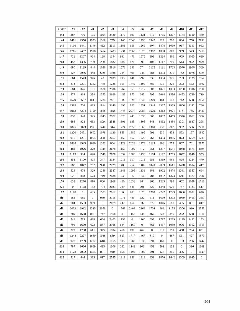
204

PORT c71 c72 d1 d2 d3 d4 d5 d6 d7 d8 d9 d10 d11 d12

c43 287 796 105 1094 2420 1176 593 1131 716 1735 1307 1174 1510 440

c44 1471 2350 1953 1366 759 1146 2040 1790 1342 323 790 884 750 2193

c45 1136 1441 1146 432 2511 1181 658 1269 807 1478 1050 917 1313 952

c46 1716 2467 1978 1454 1483 1231 2065 1875 1387 1000 809 969 573 2218

c47 721 1267 964 188 1154 931 476 1575 392 1234 806 669 1065 629

c48 457 1336 739 250 1832 588 826 590 103 1147 719 514 922 979

c49 680 1139 844 1020 2816 1572 356 574 1112 2131 1703 1570 1906 509

c50 127 2056 448 659 1988 744 496 746 284 1303 875 742 1078 649

c51 664 1543 946 43 2039 795 641 797 335 1354 926 793 1129 794

c52 814 2201 1362 778 1236 555 1442 1199 485 430 326 293 562 1602

c53 684 846 191 1180 2506 1262 353 1217 802 1821 1393 1260 1596 200

c54 877 964 384 1373 2699 1455 872 642 795 2014 1586 1453 1789 719

c55 1529 3687 1811 1224 901 1009 1898 1648 1200 181 648 742 608 2051

c56 1318 700 825 1814 3140 1896 923 1851 1348 2367 1939 1806 2142 786

c57 1912 4294 2190 1666 1695 1443 2277 2087 1579 1212 1021 1181 785 2430

c58 838 340 345 1243 2572 1328 443 1330 868 1887 1459 1326 1662 306

c59 686 928 633 809 2548 1301 145 1305 843 1862 1434 1301 1637 298

c60 1875 3023 1971 1447 344 1224 2058 1868 1360 738 802 962 566 2211

c61 1320 2491 1602 1078 1130 855 1689 1499 991 230 433 593 197 1842

c62 915 1291 1055 388 2467 1459 567 1225 763 1434 1006 873 1269 1205

c63 1828 2943 1636 1352 604 1129 2023 1773 1125 306 773 867 701 2176

c64 482 1026 320 1349 2678 1156 1002 512 754 1297 1551 1078 1474 849

c65 1113 934 620 1549 2878 1634 1386 1430 1174 2192 1765 1632 1848 955

c66 858 1100 805 347 2134 1011 317 1013 551 1389 961 828 1224 470

c67 588 1047 752 928 2729 1480 264 1482 1020 2039 1611 1478 1814 417

c68 529 674 329 1258 2587 1343 1095 1139 883 1902 1474 1341 1557 664

c69 626 868 573 749 2488 1243 85 1245 783 1002 1374 1241 1577 238

c70 638 1270 810 860 1968 400 1058 244 360 1223 795 662 1058 1711

c71 0 1178 182 704 2033 789 541 791 329 1348 920 787 1123 517

c72 1178 0 685 1583 2912 1668 783 1670 1208 2227 1799 1666 2002 646

d1 182 685 0 989 2315 1071 488 622 611 1630 1202 1069 1405 335

d2 704 1583 989 0 2079 747 664 837 375 1046 618 485 881 817

d3 2033 2912 2315 2079 0 1568 2403 2166 1704 669 1155 1306 910 2555

d4 789 1668 1071 747 1568 0 1158 644 460 823 395 262 658 1311

d5 541 783 488 664 2403 1158 0 1160 698 1717 1289 1149 1492 153

d6 791 1670 622 837 2166 644 1160 0 462 1467 1039 906 1302 1313

d7 329 1208 611 375 1704 460 698 462 0 819 591 458 794 851

d8 1348 2227 1630 1046 669 823 1717 1467 819 0 467 561 427 1870

d9 920 1799 1202 618 1155 395 1289 1039 591 467 0 133 236 1442

d10 787 1666 1069 485 1306 262 1149 906 458 561 133 0 396 1309

d11 1123 2002 1405 881 910 658 1492 1302 794 427 245 396 0 1645

d12 517 646 335 817 2555 1311 153 1313 851 1870 1442 1309 1645 0

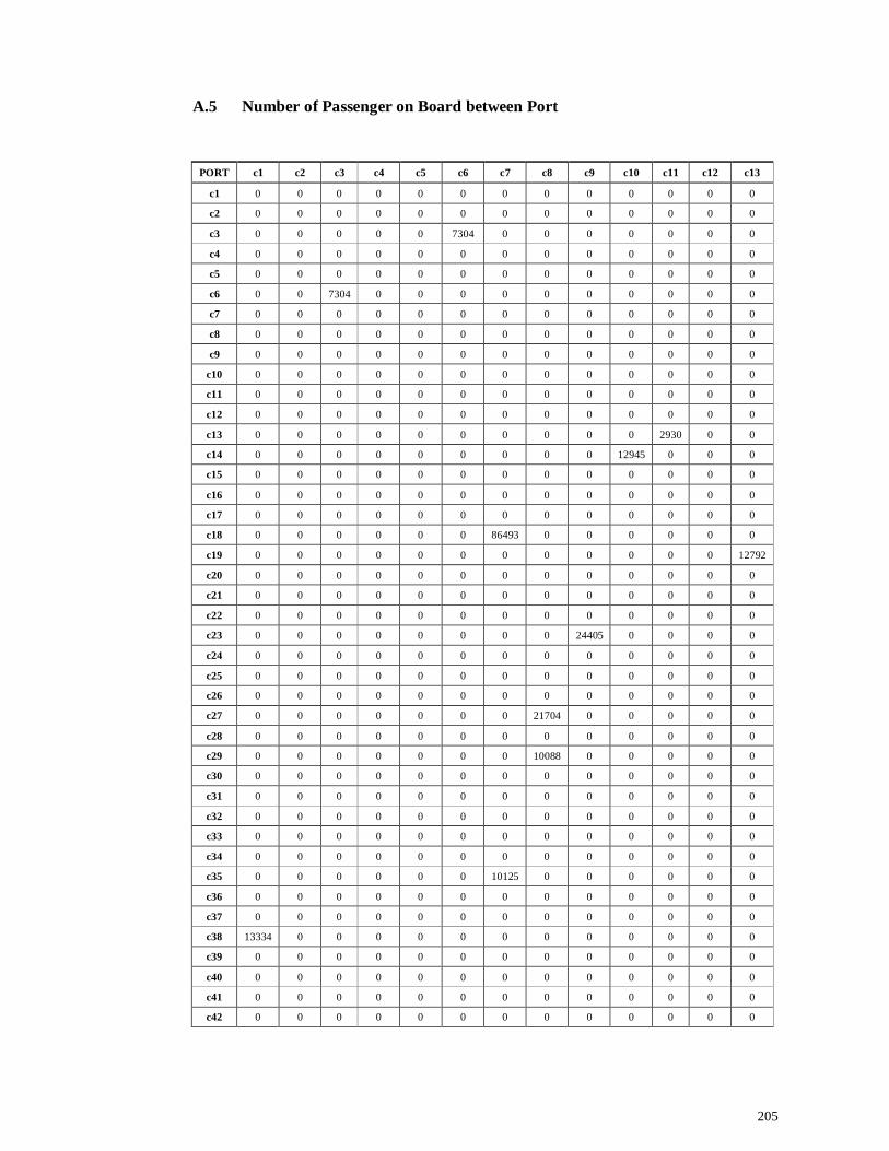
205

A.5 Number of Passenger on Board between Port

PORT c1 c2 c3 c4 c5 c6 c7 c8 c9 c10 c11 c12 c13

c1 0 0 0 0 0 0 0 0 0 0 0 0 0

c2 0 0 0 0 0 0 0 0 0 0 0 0 0

c3 0 0 0 0 0 7304 0 0 0 0 0 0 0

c4 0 0 0 0 0 0 0 0 0 0 0 0 0

c5 0 0 0 0 0 0 0 0 0 0 0 0 0

c6 0 0 7304 0 0 0 0 0 0 0 0 0 0

c7 0 0 0 0 0 0 0 0 0 0 0 0 0

c8 0 0 0 0 0 0 0 0 0 0 0 0 0

c9 0 0 0 0 0 0 0 0 0 0 0 0 0

c10 0 0 0 0 0 0 0 0 0 0 0 0 0

c11 0 0 0 0 0 0 0 0 0 0 0 0 0

c12 0 0 0 0 0 0 0 0 0 0 0 0 0

c13 0 0 0 0 0 0 0 0 0 0 2930 0 0

c14 0 0 0 0 0 0 0 0 0 12945 0 0 0

c15 0 0 0 0 0 0 0 0 0 0 0 0 0

c16 0 0 0 0 0 0 0 0 0 0 0 0 0

c17 0 0 0 0 0 0 0 0 0 0 0 0 0

c18 0 0 0 0 0 0 86493 0 0 0 0 0 0

c19 0 0 0 0 0 0 0 0 0 0 0 0 12792

c20 0 0 0 0 0 0 0 0 0 0 0 0 0

c21 0 0 0 0 0 0 0 0 0 0 0 0 0

c22 0 0 0 0 0 0 0 0 0 0 0 0 0

c23 0 0 0 0 0 0 0 0 24405 0 0 0 0

c24 0 0 0 0 0 0 0 0 0 0 0 0 0

c25 0 0 0 0 0 0 0 0 0 0 0 0 0

c26 0 0 0 0 0 0 0 0 0 0 0 0 0

c27 0 0 0 0 0 0 0 21704 0 0 0 0 0

c28 0 0 0 0 0 0 0 0 0 0 0 0 0

c29 0 0 0 0 0 0 0 10088 0 0 0 0 0

c30 0 0 0 0 0 0 0 0 0 0 0 0 0

c31 0 0 0 0 0 0 0 0 0 0 0 0 0

c32 0 0 0 0 0 0 0 0 0 0 0 0 0

c33 0 0 0 0 0 0 0 0 0 0 0 0 0

c34 0 0 0 0 0 0 0 0 0 0 0 0 0

c35 0 0 0 0 0 0 10125 0 0 0 0 0 0

c36 0 0 0 0 0 0 0 0 0 0 0 0 0

c37 0 0 0 0 0 0 0 0 0 0 0 0 0

c38 13334 0 0 0 0 0 0 0 0 0 0 0 0

c39 0 0 0 0 0 0 0 0 0 0 0 0 0

c40 0 0 0 0 0 0 0 0 0 0 0 0 0

c41 0 0 0 0 0 0 0 0 0 0 0 0 0

c42 0 0 0 0 0 0 0 0 0 0 0 0 0

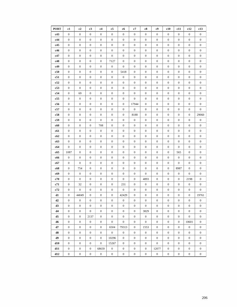
206

PORT c1 c2 c3 c4 c5 c6 c7 c8 c9 c10 c11 c12 c13

c43 0 0 0 0 0 0 0 0 0 0 0 0 0

c44 0 0 0 0 0 0 0 0 0 0 0 0 0

c45 0 0 0 0 0 0 0 0 0 0 0 0 0

c46 0 0 0 0 0 0 0 0 0 0 0 0 0

c47 0 0 0 0 0 0 0 0 0 0 0 0 0

c48 0 0 0 0 7127 0 0 0 0 0 0 0 0

c49 0 0 0 0 0 0 0 0 0 0 0 0 0

c50 0 0 0 0 0 5418 0 0 0 0 0 0 0

c51 0 0 0 0 0 0 0 0 0 0 0 0 0

c52 0 0 0 0 0 0 0 0 0 0 0 0 0

c53 0 0 0 0 0 0 0 0 0 0 0 0 0

c54 0 69 0 0 0 0 0 0 0 0 0 0 0

c55 0 0 0 0 0 0 0 0 0 0 0 0 0

c56 0 0 0 0 0 0 17944 0 0 0 0 0 0

c57 0 0 0 0 0 0 0 0 0 0 0 0 0

c58 0 0 0 0 0 0 8188 0 0 0 0 0 29060

c59 0 0 0 0 0 0 0 0 0 0 0 0 0

c60 0 0 0 708 0 0 0 0 0 0 0 0 0

c61 0 0 0 0 0 0 0 0 0 0 0 0 0

c62 0 0 0 0 0 0 0 0 0 0 0 0 0

c63 0 0 0 0 0 0 0 0 0 0 0 0 0

c64 0 0 0 0 0 0 0 0 0 0 0 0 0

c65 1087 0 0 0 0 0 0 0 0 0 565 0 0

c66 0 0 0 0 0 0 0 0 0 0 0 0 0

c67 0 0 0 0 0 0 0 0 0 0 0 0 0

c68 0 754 0 0 0 0 0 0 0 0 8987 0 0

c69 0 0 0 0 0 0 0 0 0 0 0 0 0

c70 0 0 0 0 0 0 0 4893 0 0 0 2198 0

c71 0 32 0 0 0 231 0 0 0 0 0 0 0

c72 0 0 0 0 0 0 0 0 0 0 0 0 0

d1 0 44049 0 0 0 42429 0 0 0 0 0 0 19761

d2 0 0 0 0 0 0 0 0 0 0 0 0 0

d3 0 0 0 0 0 0 0 0 0 0 0 0 0

d4 0 0 0 0 0 0 0 3829 0 0 0 0 0

d5 0 0 2137 0 0 0 0 0 0 0 0 0 0

d6 0 0 0 0 0 0 0 0 0 0 0 10601 0

d7 0 0 0 0 6504 79313 0 1553 0 0 0 0 0

d8 0 0 0 0 0 0 0 0 0 0 0 0 0

d9 0 0 0 0 10296 0 0 0 0 0 0 0 0

d10 0 0 0 0 15267 0 0 0 0 0 0 0 0

d11 0 0 0 68659 0 0 0 0 12077 0 0 0 0

d12 0 0 0 0 0 0 0 0 0 0 0 0 0

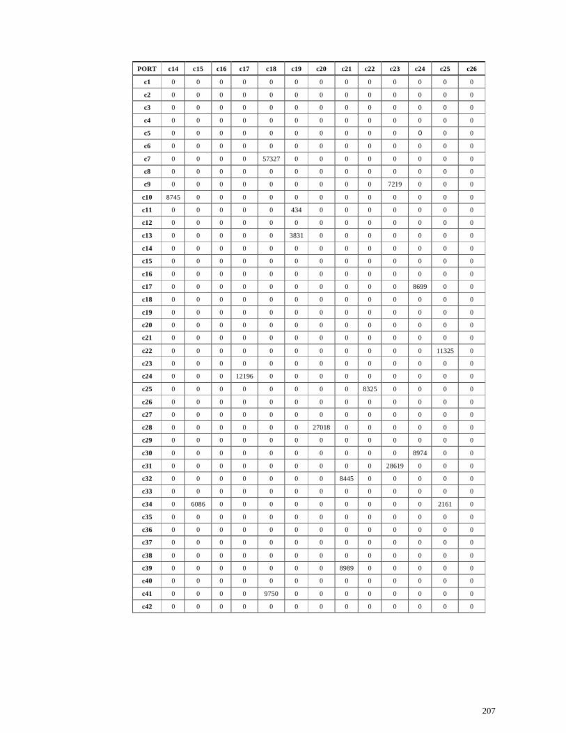
207

PORT c14 c15 c16 c17 c18 c19 c20 c21 c22 c23 c24 c25 c26

c1 0 0 0 0 0 0 0 0 0 0 0 0 0

c2 0 0 0 0 0 0 0 0 0 0 0 0 0

c3 0 0 0 0 0 0 0 0 0 0 0 0 0

c4 0 0 0 0 0 0 0 0 0 0 0 0 0

c5 0 0 0 0 0 0 0 0 0 0 0 0 0

c6 0 0 0 0 0 0 0 0 0 0 0 0 0

c7 0 0 0 0 57327 0 0 0 0 0 0 0 0

c8 0 0 0 0 0 0 0 0 0 0 0 0 0

c9 0 0 0 0 0 0 0 0 0 7219 0 0 0

c10 8745 0 0 0 0 0 0 0 0 0 0 0 0

c11 0 0 0 0 0 434 0 0 0 0 0 0 0

c12 0 0 0 0 0 0 0 0 0 0 0 0 0

c13 0 0 0 0 0 3831 0 0 0 0 0 0 0

c14 0 0 0 0 0 0 0 0 0 0 0 0 0

c15 0 0 0 0 0 0 0 0 0 0 0 0 0

c16 0 0 0 0 0 0 0 0 0 0 0 0 0

c17 0 0 0 0 0 0 0 0 0 0 8699 0 0

c18 0 0 0 0 0 0 0 0 0 0 0 0 0

c19 0 0 0 0 0 0 0 0 0 0 0 0 0

c20 0 0 0 0 0 0 0 0 0 0 0 0 0

c21 0 0 0 0 0 0 0 0 0 0 0 0 0

c22 0 0 0 0 0 0 0 0 0 0 0 11325 0

c23 0 0 0 0 0 0 0 0 0 0 0 0 0

c24 0 0 0 12196 0 0 0 0 0 0 0 0 0

c25 0 0 0 0 0 0 0 0 8325 0 0 0 0

c26 0 0 0 0 0 0 0 0 0 0 0 0 0

c27 0 0 0 0 0 0 0 0 0 0 0 0 0

c28 0 0 0 0 0 0 27018 0 0 0 0 0 0

c29 0 0 0 0 0 0 0 0 0 0 0 0 0

c30 0 0 0 0 0 0 0 0 0 0 8974 0 0

c31 0 0 0 0 0 0 0 0 0 28619 0 0 0

c32 0 0 0 0 0 0 0 8445 0 0 0 0 0

c33 0 0 0 0 0 0 0 0 0 0 0 0 0

c34 0 6086 0 0 0 0 0 0 0 0 0 2161 0

c35 0 0 0 0 0 0 0 0 0 0 0 0 0

c36 0 0 0 0 0 0 0 0 0 0 0 0 0

c37 0 0 0 0 0 0 0 0 0 0 0 0 0

c38 0 0 0 0 0 0 0 0 0 0 0 0 0

c39 0 0 0 0 0 0 0 8989 0 0 0 0 0

c40 0 0 0 0 0 0 0 0 0 0 0 0 0

c41 0 0 0 0 9750 0 0 0 0 0 0 0 0

c42 0 0 0 0 0 0 0 0 0 0 0 0 0

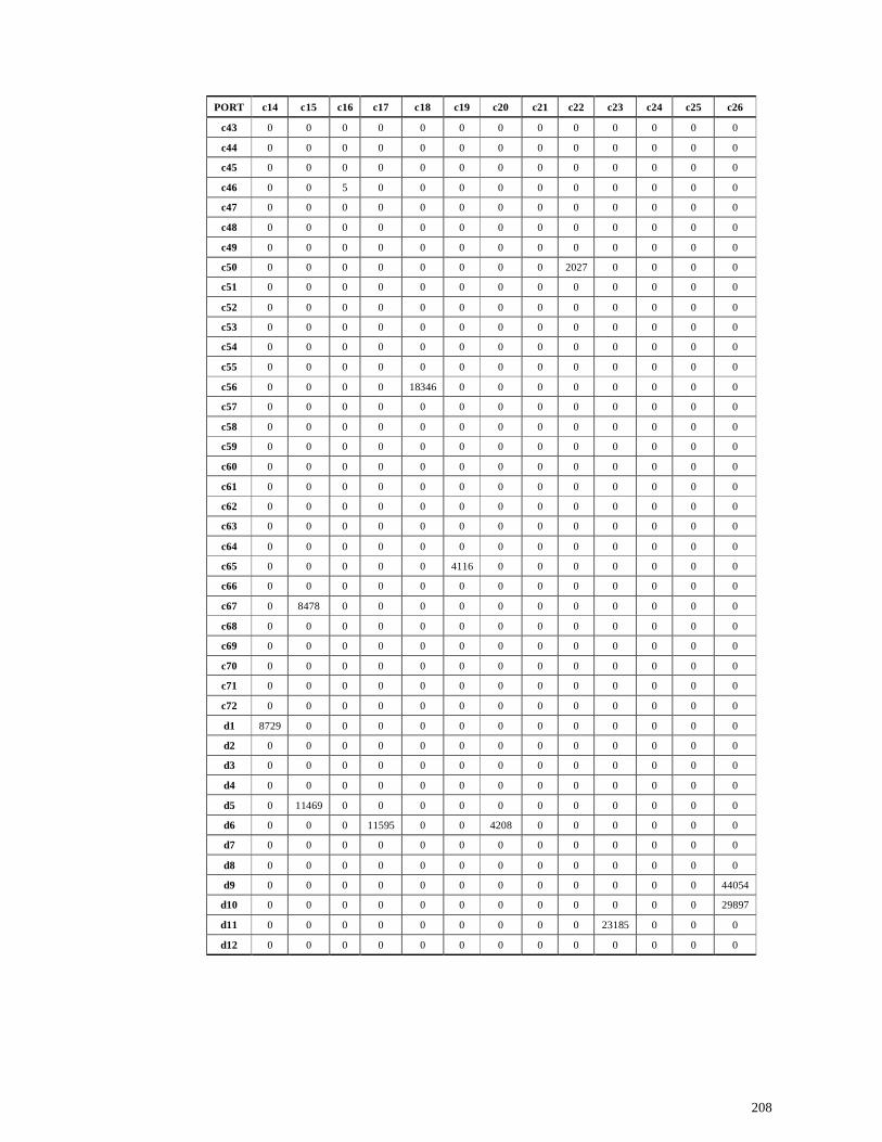
208

PORT c14 c15 c16 c17 c18 c19 c20 c21 c22 c23 c24 c25 c26

c43 0 0 0 0 0 0 0 0 0 0 0 0 0

c44 0 0 0 0 0 0 0 0 0 0 0 0 0

c45 0 0 0 0 0 0 0 0 0 0 0 0 0

c46 0 0 5 0 0 0 0 0 0 0 0 0 0

c47 0 0 0 0 0 0 0 0 0 0 0 0 0

c48 0 0 0 0 0 0 0 0 0 0 0 0 0

c49 0 0 0 0 0 0 0 0 0 0 0 0 0

c50 0 0 0 0 0 0 0 0 2027 0 0 0 0

c51 0 0 0 0 0 0 0 0 0 0 0 0 0

c52 0 0 0 0 0 0 0 0 0 0 0 0 0

c53 0 0 0 0 0 0 0 0 0 0 0 0 0

c54 0 0 0 0 0 0 0 0 0 0 0 0 0

c55 0 0 0 0 0 0 0 0 0 0 0 0 0

c56 0 0 0 0 18346 0 0 0 0 0 0 0 0

c57 0 0 0 0 0 0 0 0 0 0 0 0 0

c58 0 0 0 0 0 0 0 0 0 0 0 0 0

c59 0 0 0 0 0 0 0 0 0 0 0 0 0

c60 0 0 0 0 0 0 0 0 0 0 0 0 0

c61 0 0 0 0 0 0 0 0 0 0 0 0 0

c62 0 0 0 0 0 0 0 0 0 0 0 0 0

c63 0 0 0 0 0 0 0 0 0 0 0 0 0

c64 0 0 0 0 0 0 0 0 0 0 0 0 0

c65 0 0 0 0 0 4116 0 0 0 0 0 0 0

c66 0 0 0 0 0 0 0 0 0 0 0 0 0

c67 0 8478 0 0 0 0 0 0 0 0 0 0 0

c68 0 0 0 0 0 0 0 0 0 0 0 0 0

c69 0 0 0 0 0 0 0 0 0 0 0 0 0

c70 0 0 0 0 0 0 0 0 0 0 0 0 0

c71 0 0 0 0 0 0 0 0 0 0 0 0 0

c72 0 0 0 0 0 0 0 0 0 0 0 0 0

d1 8729 0 0 0 0 0 0 0 0 0 0 0 0

d2 0 0 0 0 0 0 0 0 0 0 0 0 0

d3 0 0 0 0 0 0 0 0 0 0 0 0 0

d4 0 0 0 0 0 0 0 0 0 0 0 0 0

d5 0 11469 0 0 0 0 0 0 0 0 0 0 0

d6 0 0 0 11595 0 0 4208 0 0 0 0 0 0

d7 0 0 0 0 0 0 0 0 0 0 0 0 0

d8 0 0 0 0 0 0 0 0 0 0 0 0 0

d9 0 0 0 0 0 0 0 0 0 0 0 0 44054

d10 0 0 0 0 0 0 0 0 0 0 0 0 29897

d11 0 0 0 0 0 0 0 0 0 23185 0 0 0

d12 0 0 0 0 0 0 0 0 0 0 0 0 0

209

PORT c27 c28 c29 c30 c31 c32 c33 c34 c35 c36 c37 c38 c39

c1 0 0 0 0 0 0 0 0 0 0 0 7333 0

c2 0 0 0 0 0 0 0 0 0 0 0 0 0

c3 0 0 0 0 0 0 0 0 0 0 0 0 0

c4 0 0 0 0 0 0 0 0 0 0 0 0 0

c5 0 0 0 0 0 0 0 0 0 0 0 0 0

c6 0 0 0 0 0 0 0 0 0 0 0 0 0

c7 0 0 0 0 0 0 0 0 10028 0 0 0 0

c8 21704 0 8318 0 0 0 0 0 0 0 0 0 0

c9 0 0 0 0 0 0 0 0 0 0 0 0 0

c10 0 0 0 0 0 0 0 0 0 0 0 0 0

c11 0 0 0 0 0 0 0 0 0 0 0 0 0

c12 0 0 0 0 0 0 0 0 0 0 0 0 0

c13 0 0 0 0 0 0 0 0 0 0 0 0 0

c14 0 0 0 0 0 0 0 0 0 0 0 0 0

c15 0 0 0 0 0 0 0 6086 0 0 0 0 0

c16 0 0 0 0 0 0 0 0 0 0 0 0 0

c17 0 0 0 0 0 0 0 0 0 0 0 0 0

c18 0 0 0 0 0 0 0 0 0 0 0 0 0

c19 0 0 0 0 0 0 0 0 0 0 0 0 0

c20 0 2505 0 0 0 0 0 0 0 0 0 0 0

c21 0 0 0 0 0 2459 0 0 0 0 0 0 6763

c22 0 0 0 0 0 0 0 0 0 0 0 0 0

c23 0 0 0 0 28619 0 0 0 0 0 0 0 0

c24 0 0 0 8961 0 0 0 0 0 0 0 0 0

c25 0 0 0 0 0 0 0 2517 0 0 0 0 0

c26 0 0 0 0 0 0 0 0 0 0 0 0 0

c27 0 0 0 0 0 0 0 0 0 3122 0 0 0

c28 0 0 0 0 0 0 0 0 0 0 0 0 0

c29 0 0 0 0 0 0 0 0 0 0 0 0 0

c30 0 0 0 0 0 0 0 0 0 0 0 0 0

c31 0 0 0 0 0 0 0 0 0 0 0 0 0

c32 0 0 0 0 0 0 0 0 0 0 0 0 0

c33 0 0 0 0 0 0 0 0 0 0 108290 0 0

c34 0 0 0 0 0 0 0 0 0 0 0 0 0

c35 0 0 0 0 0 0 0 0 0 0 0 0 0

c36 3122 0 0 0 0 0 0 0 0 0 5028 0 0

c37 0 0 0 0 0 0 109613 0 0 5028 0 0 0

c38 0 0 0 0 0 0 0 0 0 0 0 0 0

c39 0 0 0 0 0 0 0 0 0 0 0 0 0

c40 0 0 0 0 0 0 0 0 0 0 0 0 0

c41 0 0 0 0 0 0 0 0 33830 0 0 0 0

c42 0 0 0 0 0 0 0 0 0 0 0 0 0

210

PORT c27 c28 c29 c30 c31 c32 c33 c34 c35 c36 c37 c38 c39

c43 0 0 0 0 0 0 0 0 0 0 0 0 0

c44 0 0 0 0 0 0 0 0 0 0 0 0 0

c45 0 0 0 0 0 0 0 0 0 0 0 0 0

c46 0 0 0 0 0 0 0 0 0 0 0 0 0

c47 0 0 0 0 0 0 0 0 0 0 0 0 0

c48 0 0 0 0 0 0 0 0 0 0 0 0 0

c49 0 0 0 0 0 0 0 0 0 0 0 0 0

c50 0 0 0 0 0 0 0 0 0 0 0 0 0

c51 0 0 0 0 0 0 0 0 0 0 0 0 0

c52 0 0 0 0 0 0 0 0 0 0 0 0 0

c53 0 0 0 0 0 0 0 0 0 0 0 0 0

c54 0 0 0 0 0 0 0 0 0 0 0 0 0

c55 0 0 0 0 0 0 0 0 0 0 0 0 0

c56 0 0 0 0 0 0 0 0 0 0 0 0 0

c57 0 0 0 0 0 0 0 0 0 0 0 0 0

c58 0 0 0 0 0 0 0 0 43140 0 0 0 0

c59 0 0 0 0 0 2159 0 0 0 0 0 0 0

c60 0 0 0 0 0 0 0 0 0 0 0 0 0

c61 0 0 0 0 0 0 0 0 0 0 0 0 0

c62 0 0 0 0 0 0 0 0 0 0 0 0 0

c63 0 0 0 0 2373 0 0 0 0 0 0 0 0

c64 0 0 0 9532 0 0 0 0 0 0 0 0 0

c65 0 0 0 0 0 0 0 0 0 0 0 0 0

c66 0 0 0 0 0 0 0 0 0 0 0 0 0

c67 0 0 0 0 0 0 0 0 0 0 0 0 0

c68 0 0 0 0 0 0 0 0 0 0 0 0 0

c69 0 0 0 0 0 0 0 0 0 0 0 0 0

c70 0 0 0 0 0 0 0 0 0 0 0 0 0

c71 0 0 0 0 0 0 0 0 0 0 0 0 0

c72 0 0 0 0 0 0 0 0 3872 0 0 0 0

d1 0 0 0 0 0 0 0 0 0 0 0 0 0

d2 0 0 0 0 0 0 0 0 0 0 0 0 0

d3 0 0 0 0 0 0 0 0 0 0 0 0 0

d4 0 0 12494 0 0 0 0 0 0 0 0 0 0

d5 0 0 0 0 0 0 0 0 0 0 0 0 0

d6 0 9493 0 0 0 0 77927 0 0 0 0 0 0

d7 1275 13730 0 0 0 0 0 0 0 0 20408 0 0

d8 0 0 0 0 0 0 0 0 0 0 0 0 0

d9 0 0 0 0 0 0 0 0 0 0 0 0 0

d10 0 0 0 0 0 0 0 0 0 0 0 0 0

d11 0 0 0 0 0 0 0 0 0 0 0 0 0

d12 0 0 0 0 0 0 0 0 0 0 0 0 0

211

PORT c40 c41 c42 c43 c44 c45 c46 c47 c48 c49 c50 c51 c52 c1 0 0 0 0 0 0 0 0 0 0 0 0 0 c2 0 0 0 0 0 0 0 0 0 0 0 0 0 c3 0 0 0 0 0 0 0 0 0 0 0 0 0 c4 0 0 0 0 0 0 0 0 0 0 0 0 0 c5 0 0 0 0 0 0 0 0 4828 0 0 0 0 c6 0 0 0 0 0 0 0 0 0 0 5418 0 0 c7 0 0 0 0 0 0 0 0 0 0 0 0 0 c8 0 0 0 0 0 0 0 0 0 0 0 0 0 c9 0 0 0 0 0 0 0 0 0 0 0 0 0

c10 0 0 0 0 0 0 0 0 0 0 0 0 0 c11 0 0 0 0 0 0 0 0 0 0 0 0 0 c12 0 0 0 0 0 0 0 0 0 0 0 0 0 c13 0 0 0 0 0 0 0 0 0 0 0 0 0 c14 0 0 0 0 0 0 0 0 0 0 0 0 0 c15 0 0 0 0 0 0 0 0 0 0 0 0 0 c16 0 0 0 0 0 0 0 0 0 0 0 0 0 c17 0 0 0 0 0 0 0 0 0 0 0 0 0 c18 0 33775 0 0 0 0 0 0 0 0 0 0 0 c19 0 0 0 0 0 0 0 0 0 0 0 0 0 c20 0 0 0 0 0 0 0 0 0 0 0 0 0 c21 0 0 0 0 0 0 0 0 0 0 0 0 0 c22 0 0 0 0 0 0 0 0 0 0 2027 0 0 c23 0 0 0 0 0 0 0 0 0 0 0 0 0 c24 0 0 0 0 0 0 0 0 0 0 0 0 0 c25 0 0 0 0 0 0 0 0 0 0 0 0 0 c26 0 0 0 0 0 0 0 0 0 0 0 0 0 c27 0 0 0 0 0 0 0 0 0 0 0 0 0 c28 0 0 0 0 0 0 0 0 0 0 0 0 0 c29 0 0 0 0 0 0 0 0 0 0 0 0 0 c30 0 0 0 0 0 0 0 0 0 0 0 0 0 c31 0 0 0 0 0 0 0 0 0 0 0 0 0 c32 0 0 0 0 0 0 0 0 0 0 0 0 0 c33 0 0 0 0 0 0 0 0 0 0 0 0 0 c34 0 0 0 0 0 0 0 0 0 0 0 0 0 c35 0 27530 0 0 0 0 0 0 0 0 0 0 0 c36 0 0 0 0 0 0 0 0 0 0 0 0 0 c37 0 0 0 0 0 0 0 0 0 0 0 0 0 c38 0 0 0 0 0 0 0 0 0 0 0 0 0 c39 0 0 0 0 0 0 0 0 0 0 0 0 0 c40 0 0 0 0 4391 0 0 0 0 0 0 0 0 c41 0 0 0 0 0 0 0 0 0 0 0 0 0 c42 0 0 0 0 0 0 0 0 0 0 0 0 0

212

PORT c40 c41 c42 c43 c44 c45 c46 c47 c48 c49 c50 c51 c52

c43 0 0 0 0 0 0 0 0 0 0 0 0 0

c44 4391 0 0 0 0 0 0 0 0 0 0 0 0

c45 0 0 0 0 0 0 0 3590 12347 0 0 0 0

c46 0 0 0 0 0 0 0 0 0 0 0 0 0

c47 0 0 0 0 0 3590 0 0 5094 0 0 0 0

c48 0 0 0 0 0 0 0 5094 0 0 0 9857 0

c49 0 0 0 0 0 0 0 0 0 0 0 0 0

c50 0 0 0 0 0 0 0 0 0 0 0 0 0

c51 0 0 0 0 0 0 0 0 5458 0 0 0 0

c52 0 0 0 0 0 0 0 0 0 0 0 0 0

c53 0 0 9725 0 0 0 0 0 0 0 0 0 0

c54 0 0 0 0 0 0 0 0 0 0 0 0 0

c55 687 0 0 0 0 0 0 0 0 0 0 0 0

c56 0 35983 0 0 0 0 0 0 0 0 0 0 0

c57 0 0 0 0 0 0 9 0 0 0 0 0 0

c58 0 0 0 0 0 0 0 0 0 0 0 0 0

c59 0 0 0 0 0 0 0 0 0 0 0 0 0

c60 0 0 0 0 0 0 0 0 0 0 0 0 0

c61 0 0 0 0 0 0 0 0 0 0 0 0 0

c62 0 0 0 0 0 77062 0 0 0 0 0 0 0

c63 0 0 0 0 12287 0 0 0 0 0 0 0 0

c64 0 0 0 0 0 0 0 0 0 0 0 0 0

c65 0 0 0 0 0 0 0 0 0 0 0 0 0

c66 0 0 0 0 0 0 0 15631 0 0 0 0 0

c67 0 0 0 0 0 0 0 0 0 7937 0 0 0

c68 0 0 0 0 0 0 0 0 0 0 0 0 0

c69 0 0 0 0 0 0 0 0 0 0 0 0 0

c70 0 0 0 0 0 0 0 0 0 0 0 0 0

c71 0 0 0 0 0 0 0 0 0 0 0 0 0

c72 0 5221 0 0 0 0 0 0 0 0 0 0 0

d1 0 0 49483 8132 0 0 0 0 0 0 0 0 0

d2 0 0 0 0 0 0 0 80995 59302 0 0 0 0

d3 0 0 0 0 0 0 0 0 0 0 0 0 0

d4 0 0 0 0 0 0 0 0 0 0 0 0 0

d5 0 0 0 0 0 0 0 3050 0 0 0 0 0

d6 0 0 0 0 0 0 0 0 0 0 0 0 0

d7 0 0 0 0 0 0 0 0 19265 0 0 2502 0

d8 0 0 0 0 0 0 0 0 0 0 0 0 0

d9 0 0 0 0 0 0 0 0 0 0 0 0 32107

d10 0 0 0 0 0 0 0 0 38944 0 0 0 59258

d11 0 0 0 0 0 0 1705 0 0 0 0 0 0

d12 0 0 1267 0 0 0 0 0 0 0 0 0 0

213

PORT c53 c54 c55 c56 c57 c58 c59 c60 c61 c62 c63 c64 c65

c1 0 0 0 0 0 0 0 0 0 0 0 0 3268

c2 0 56 0 0 0 0 0 0 0 0 0 0 0

c3 0 0 0 0 0 0 0 0 0 0 0 0 0

c4 0 0 0 0 0 0 0 723 0 0 0 0 0

c5 0 0 0 0 0 0 0 0 0 0 0 0 0

c6 0 0 0 0 0 0 0 0 0 0 0 0 0

c7 0 0 0 16944 0 8188 0 0 0 0 0 0 0

c8 0 0 0 0 0 0 0 0 0 0 0 0 0

c9 0 0 0 0 0 0 0 0 0 0 0 0 0

c10 0 0 0 0 0 0 0 0 0 0 0 0 0

c11 0 0 0 0 0 0 0 0 0 0 0 0 2647

c12 0 0 0 0 0 0 0 0 0 0 0 0 0

c13 0 0 0 0 0 25610 0 0 0 0 0 0 0

c14 0 0 0 0 0 0 0 0 0 0 0 0 0

c15 0 0 0 0 0 0 0 0 0 0 0 0 0

c16 0 0 0 0 26 0 0 0 0 0 0 0 0

c17 0 0 0 0 0 0 0 0 0 0 0 0 0

c18 0 0 0 14753 0 0 0 0 0 0 0 0 0

c19 0 0 0 0 0 0 0 0 0 0 0 0 204

c20 0 0 0 0 0 0 0 0 0 0 0 0 0

c21 0 0 0 0 0 0 0 0 0 0 0 0 0

c22 0 0 0 0 0 0 0 0 0 0 0 0 0

c23 0 0 0 0 0 0 0 0 0 0 0 0 0

c24 0 0 0 0 0 0 0 0 0 0 0 0 0

c25 0 0 0 0 0 0 0 0 0 0 0 0 0

c26 0 0 0 0 0 0 0 0 0 0 0 0 0

c27 0 0 0 0 0 0 0 0 0 0 0 0 0

c28 0 0 0 0 0 0 0 0 0 0 0 0 0

c29 0 0 0 0 0 0 0 0 0 0 0 0 0

c30 0 0 0 0 0 0 0 0 0 0 0 9320 0

c31 0 0 0 0 0 0 0 0 0 0 2373 0 0

c32 0 0 0 0 0 0 8414 0 0 0 0 0 0

c33 0 0 0 0 0 0 0 0 0 0 0 0 0

c34 0 0 0 0 0 0 0 0 0 0 0 0 0

c35 0 0 0 0 0 53501 0 0 0 0 0 0 0

c36 0 0 0 0 0 0 0 0 0 0 0 0 0

c37 0 0 0 0 0 0 0 0 0 0 0 0 0

c38 0 0 0 0 0 0 0 0 0 0 0 0 0

c39 0 0 0 0 0 0 0 0 0 0 0 0 0

c40 0 0 687 0 0 0 0 0 0 0 0 0 0

c41 0 0 0 35983 0 0 0 0 0 0 0 0 0

c42 7254 0 0 0 0 0 0 0 0 0 0 0 0

214

PORT c53 c54 c55 c56 c57 c58 c59 c60 c61 c62 c63 c64 c65

c43 0 0 0 0 0 0 0 0 0 0 0 0 0

c44 0 0 0 0 0 0 0 0 0 0 12287 0 0

c45 0 0 0 0 0 0 0 0 0 6512 0 0 0

c46 0 0 0 0 0 0 0 0 0 0 0 0 0

c47 0 0 0 0 0 0 0 0 0 0 0 0 0

c48 0 0 0 0 0 0 0 0 0 0 0 0 0

c49 0 0 0 0 0 0 0 0 0 0 0 0 0

c50 0 0 0 0 0 0 0 0 0 0 0 0 0

c51 0 0 0 0 0 0 0 0 0 0 0 0 0

c52 0 0 0 0 0 0 0 0 0 0 0 0 0

c53 0 0 0 0 0 0 0 0 0 0 0 0 0

c54 0 0 0 0 0 0 0 0 0 0 0 8922 0

c55 0 0 0 0 0 0 0 0 0 0 0 0 0

c56 0 0 0 0 0 0 0 0 0 0 0 0 0

c57 0 0 0 0 0 0 0 0 0 0 0 0 0

c58 0 0 0 0 0 0 0 0 0 0 0 0 0

c59 0 0 0 0 0 0 0 0 0 0 0 0 0

c60 0 0 0 0 0 0 0 0 0 0 0 0 0

c61 0 0 0 0 0 0 0 0 0 0 0 0 0

c62 0 0 0 0 0 0 0 0 0 0 0 0 0

c63 0 0 0 0 0 0 0 0 0 0 0 0 0

c64 0 9729 0 0 0 0 0 0 0 0 0 0 0

c65 0 0 0 0 0 0 0 0 0 0 0 0 0

c66 0 0 0 0 0 0 0 0 0 13828 0 0 0

c67 0 0 0 0 0 0 0 0 0 0 0 0 0

c68 0 54 0 0 0 0 0 0 0 0 0 0 0

c69 0 0 0 0 0 0 9165 0 0 0 0 0 0

c70 0 0 0 0 0 0 0 0 0 0 0 0 0

c71 0 0 0 0 0 0 0 0 0 0 0 0 0

c72 0 0 0 0 0 0 0 0 0 0 0 0 0

d1 0 13547 0 0 0 26867 0 0 0 0 0 0 0

d2 0 0 0 0 0 0 0 0 0 8287 0 0 0

d3 0 0 0 0 0 0 0 21856 0 0 0 0 0

d4 0 0 0 0 0 0 0 0 0 0 0 0 0

d5 0 0 0 0 0 4478 0 0 0 0 0 0 0

d6 0 0 0 0 0 0 0 0 0 0 0 0 0

d7 0 0 0 0 0 22764 0 0 0 0 0 0 0

d8 0 0 21765 0 0 0 0 0 5665 0 0 0 0

d9 0 0 0 0 0 0 0 0 0 0 0 0 0

d10 0 0 0 0 0 0 0 0 0 0 0 0 0

d11 0 0 0 0 0 0 0 0 1439 0 0 0 0

d12 5943 0 0 0 0 14646 0 0 0 0 0 0 0

215

PORT c66 c67 c68 c69 c70 c71 c72 d1 d2 d3 d4 d5 d6

c1 0 0 0 0 0 0 0 0 0 0 0 0 0

c2 0 0 7406 0 0 365 0 384 0 0 0 0 0

c3 0 0 0 0 0 0 0 0 0 0 0 1983 0

c4 0 0 0 0 0 0 0 0 0 0 0 0 0

c5 0 0 0 0 0 0 0 0 0 0 0 0 0

c6 0 0 0 0 0 4121 0 55845 0 0 0 0 0

c7 0 0 0 0 0 0 0 0 0 0 0 0 0

c8 0 0 0 0 4893 0 0 0 0 0 4511 0 0

c9 0 0 0 0 0 0 0 0 0 0 0 0 0

c10 0 0 0 0 0 0 0 0 0 0 0 0 0

c11 0 0 8463 0 0 0 0 0 0 0 0 0 0

c12 0 0 0 0 2198 0 0 0 0 0 0 0 10601

c13 0 0 0 0 0 0 0 19761 0 0 0 0 0

c14 0 0 0 0 0 0 0 9718 0 0 0 0 0

c15 0 7552 0 0 0 0 0 0 0 0 0 16136 0

c16 0 0 0 0 0 0 0 0 0 0 0 0 0

c17 0 0 0 0 0 0 0 0 0 0 0 0 13165

c18 0 0 0 0 0 0 0 0 0 0 0 0 0

c19 0 0 0 0 0 0 0 0 0 0 0 0 0

c20 0 0 0 0 0 0 0 0 0 0 0 0 15479

c21 0 0 0 0 0 0 0 0 0 0 0 0 0

c22 0 0 0 0 0 0 0 0 0 0 0 0 0

c23 0 0 0 0 0 0 0 0 0 0 0 0 0

c24 0 0 0 0 0 0 0 0 0 0 0 0 0

c25 0 0 0 0 0 0 0 0 0 0 0 0 0

c26 0 0 0 0 0 0 0 0 0 0 0 0 0

c27 0 0 0 0 0 0 0 0 0 0 0 0 0

c28 0 0 0 0 0 0 0 0 0 0 0 0 9974

c29 0 0 0 0 0 0 0 0 0 0 13559 0 0

c30 0 0 0 0 0 0 0 0 0 0 0 0 0

c31 0 0 0 0 0 0 0 0 0 0 0 0 0

c32 0 0 0 0 0 0 0 0 0 0 0 0 0

c33 0 0 0 0 0 0 0 0 0 0 0 0 77857

c34 0 0 0 0 0 0 0 0 0 0 0 0 0

c35 0 0 0 0 0 0 14694 0 0 0 0 0 0

c36 0 0 0 0 0 0 0 0 0 0 0 0 0

c37 0 0 0 0 0 0 0 0 0 0 0 0 0

c38 0 0 0 0 0 0 0 0 0 0 0 0 0

c39 0 0 0 0 0 0 0 0 0 0 0 0 0

c40 0 0 0 0 0 0 0 0 0 0 0 0 0

c41 0 0 0 0 0 0 20824 0 0 0 0 0 0

c42 0 0 0 0 0 0 0 49483 0 0 0 0 0

216

PORT c66 c67 c68 c69 c70 c71 c72 d1 d2 d3 d4 d5 d6

c43 0 0 0 0 0 0 0 9776 0 0 0 0 0

c44 0 0 0 0 0 0 0 0 0 0 0 0 0

c45 13966 0 0 0 0 0 0 0 12619 0 0 0 0

c46 0 0 0 0 0 0 0 0 0 0 0 0 0

c47 17894 0 0 0 0 0 0 0 81170 0 0 3050 0

c48 0 0 0 0 0 0 0 0 155179 0 0 0 0

c49 0 9763 0 0 0 0 0 0 0 0 0 0 0

c50 0 0 0 0 0 0 0 0 0 0 0 0 0

c51 0 0 0 0 0 0 0 0 0 0 0 0 0

c52 0 0 0 0 0 0 0 0 0 0 0 0 0

c53 0 0 0 0 0 0 0 0 0 0 0 0 0

c54 0 0 84 0 0 0 0 12552 0 0 0 0 0

c55 0 0 0 0 0 0 0 0 0 0 0 0 0

c56 0 0 0 0 0 0 0 0 0 0 0 0 0

c57 0 0 0 0 0 0 0 0 0 0 0 0 0

c58 0 0 0 0 0 0 0 32912 0 0 0 935 0

c59 0 0 0 5879 0 0 0 0 0 0 0 0 0

c60 0 0 0 0 0 0 0 0 0 19856 0 0 0

c61 0 0 0 0 0 0 0 0 0 0 0 0 0

c62 0 0 0 0 0 0 0 0 3979 0 0 0 0

c63 0 0 0 0 0 0 0 0 0 0 0 0 0

c64 0 0 0 0 0 0 0 0 0 0 0 0 0

c65 0 0 0 0 0 0 0 0 0 0 0 0 0

c66 0 0 0 0 0 0 0 0 0 0 0 0 0

c67 0 0 0 0 0 0 0 0 0 0 0 0 0

c68 0 0 0 0 0 0 0 0 0 0 0 0 0

c69 0 0 0 0 0 0 0 0 0 0 0 4643 0

c70 0 0 0 0 0 0 0 0 0 0 0 0 0

c71 0 0 0 0 0 0 0 0 0 0 0 0 0

c72 0 0 0 0 0 0 0 0 0 0 0 0 0

d1 0 0 0 0 0 0 0 0 0 0 0 0 0

d2 0 0 0 0 0 0 0 0 0 0 0 0 0

d3 0 0 0 0 0 0 0 0 0 0 0 0 0

d4 0 0 0 0 0 0 0 0 0 0 0 0 0

d5 0 0 0 2121 0 0 0 0 0 0 0 0 0

d6 0 0 0 0 0 0 0 0 0 0 0 0 0

d7 0 0 0 0 0 0 0 13785 0 0 0 0 0

d8 0 0 0 0 0 0 0 0 0 0 0 0 0

d9 0 0 0 0 0 0 0 0 0 0 0 0 0

d10 0 0 0 0 0 0 0 0 35094 0 11217 0 0

d11 0 0 0 0 0 0 0 0 0 0 0 0 0

d12 0 0 0 0 0 0 0 0 0 0 0 57064 0

217

PORT d7 d8 d9 d10 d11 d12

c43 0 0 0 0 0 0

c44 0 0 0 0 0 0

c45 0 0 0 0 0 0

c46 0 0 0 0 1705 0

c47 0 0 0 0 0 0

c48 26674 0 0 1605 0 0

c49 0 0 0 0 0 0

c50 0 0 0 0 0 0

c51 6112 0 0 0 0 0

c52 0 0 16296 59116 0 0

c53 0 0 0 0 0 1878

c54 0 0 0 0 0 0

c55 0 339 0 0 0 0

c56 0 0 0 0 0 0

c57 0 0 0 0 0 0

c58 12973 0 0 0 0 14646

c59 0 0 0 0 0 0

c60 0 0 0 0 0 0

c61 0 3 0 0 5705 0

c62 0 0 0 0 0 0

c63 0 0 0 0 0 0

c64 0 0 0 0 0 0

c65 0 0 0 0 0 0

c66 0 0 0 0 0 0

c67 0 0 0 0 0 0

c68 0 0 0 0 0 0

c69 0 0 0 0 0 0

c70 0 0 0 0 0 0

c71 0 0 0 0 0 0

c72 0 0 0 0 0 0

d1 4790 0 0 0 0 0

d2 0 0 0 8475 0 0

d3 0 0 0 0 0 0

d4 0 0 0 4613 0 0

d5 0 0 0 0 0 74195

d6 0 0 0 0 0 0

d7 0 0 0 75258 5075 0

d8 0 0 15392 8032 0 0

d9 9209 20842 0 0 1149 0

d10 130994 47825 0 0 8327 0

d11 0 0 18725 41075 0 0

d12 0 0 0 0 0 0

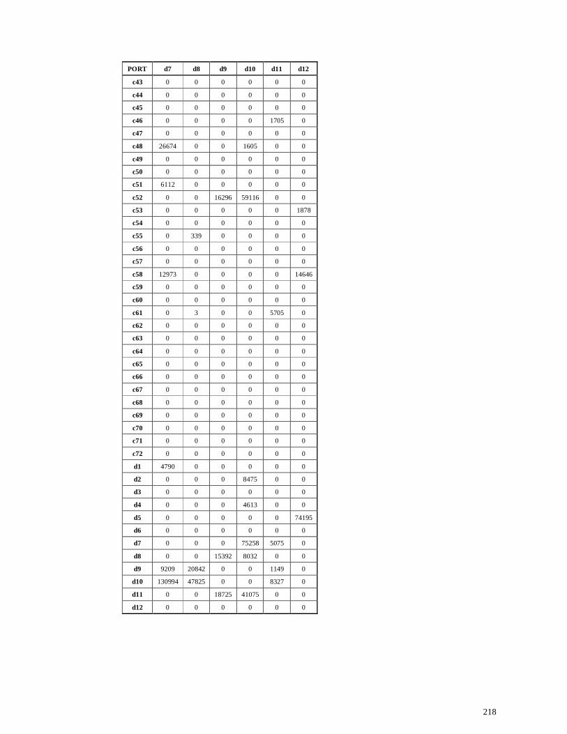
218

PORT d7 d8 d9 d10 d11 d12

c43 0 0 0 0 0 0

c44 0 0 0 0 0 0

c45 0 0 0 0 0 0

c46 0 0 0 0 1705 0

c47 0 0 0 0 0 0

c48 26674 0 0 1605 0 0

c49 0 0 0 0 0 0

c50 0 0 0 0 0 0

c51 6112 0 0 0 0 0

c52 0 0 16296 59116 0 0

c53 0 0 0 0 0 1878

c54 0 0 0 0 0 0

c55 0 339 0 0 0 0

c56 0 0 0 0 0 0

c57 0 0 0 0 0 0

c58 12973 0 0 0 0 14646

c59 0 0 0 0 0 0

c60 0 0 0 0 0 0

c61 0 3 0 0 5705 0

c62 0 0 0 0 0 0

c63 0 0 0 0 0 0

c64 0 0 0 0 0 0

c65 0 0 0 0 0 0

c66 0 0 0 0 0 0

c67 0 0 0 0 0 0

c68 0 0 0 0 0 0

c69 0 0 0 0 0 0

c70 0 0 0 0 0 0

c71 0 0 0 0 0 0

c72 0 0 0 0 0 0

d1 4790 0 0 0 0 0

d2 0 0 0 8475 0 0

d3 0 0 0 0 0 0

d4 0 0 0 4613 0 0

d5 0 0 0 0 0 74195

d6 0 0 0 0 0 0

d7 0 0 0 75258 5075 0

d8 0 0 15392 8032 0 0

d9 9209 20842 0 0 1149 0

d10 130994 47825 0 0 8327 0

d11 0 0 18725 41075 0 0

d12 0 0 0 0 0 0

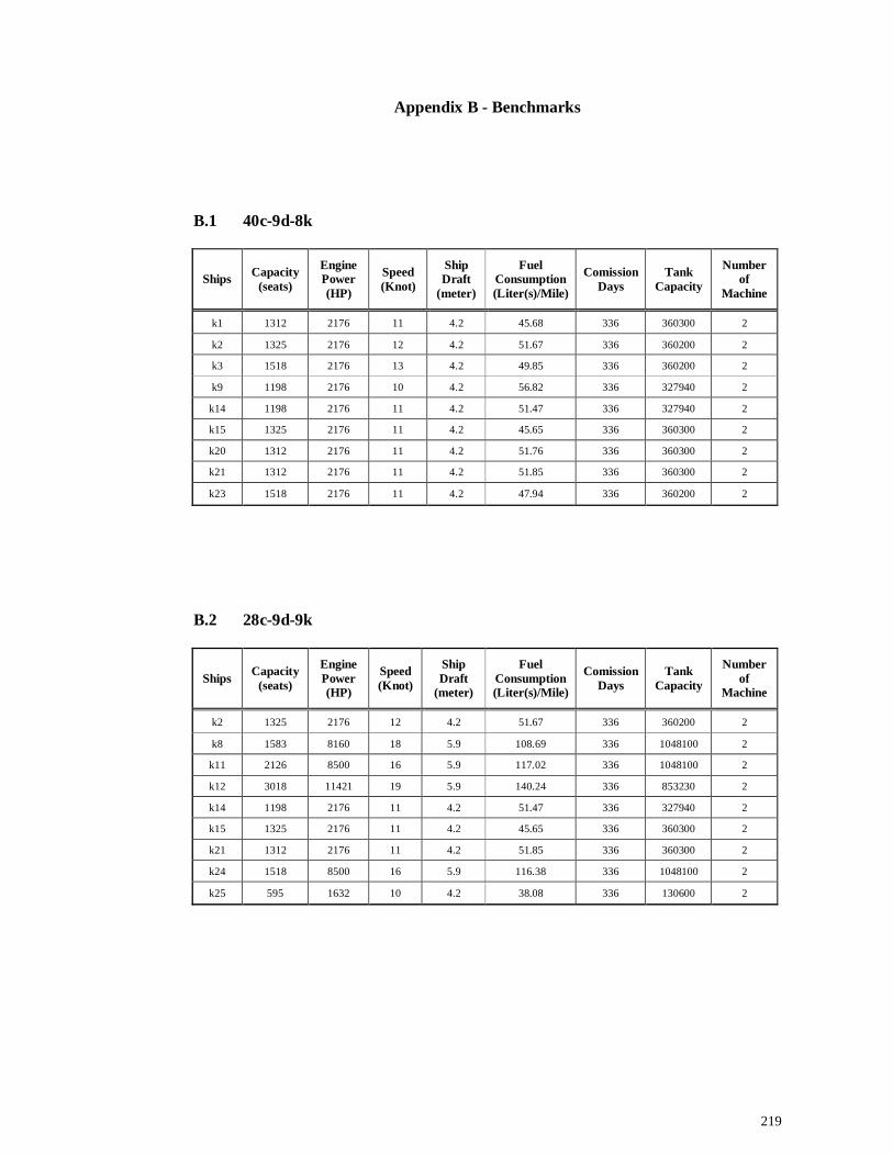
219

Appendix B - Benchmarks

B.1 40c-9d-8k

Ships Capacity (seats)

Engine Power (HP)

Speed (Knot)

Ship Draft

(meter)

Fuel Consumption (Liter(s)/Mile)

Comission Days

Tank Capacity

Number of

Machine

k1 1312 2176 11 4.2 45.68 336 360300 2

k2 1325 2176 12 4.2 51.67 336 360200 2

k3 1518 2176 13 4.2 49.85 336 360200 2

k9 1198 2176 10 4.2 56.82 336 327940 2

k14 1198 2176 11 4.2 51.47 336 327940 2

k15 1325 2176 11 4.2 45.65 336 360300 2

k20 1312 2176 11 4.2 51.76 336 360300 2

k21 1312 2176 11 4.2 51.85 336 360300 2

k23 1518 2176 11 4.2 47.94 336 360200 2

B.2 28c-9d-9k

Ships Capacity (seats)

Engine Power (HP)

Speed (Knot)

Ship Draft

(meter)

Fuel Consumption (Liter(s)/Mile)

Comission Days

Tank Capacity

Number of

Machine

k2 1325 2176 12 4.2 51.67 336 360200 2

k8 1583 8160 18 5.9 108.69 336 1048100 2

k11 2126 8500 16 5.9 117.02 336 1048100 2

k12 3018 11421 19 5.9 140.24 336 853230 2

k14 1198 2176 11 4.2 51.47 336 327940 2

k15 1325 2176 11 4.2 45.65 336 360300 2

k21 1312 2176 11 4.2 51.85 336 360300 2

k24 1518 8500 16 5.9 116.38 336 1048100 2

k25 595 1632 10 4.2 38.08 336 130600 2

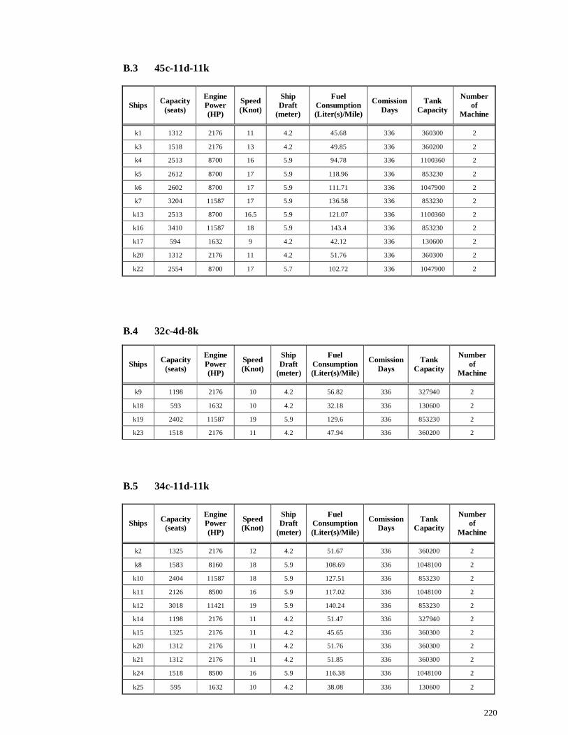
220

B.3 45c-11d-11k

Ships Capacity (seats)

Engine Power (HP)

Speed (Knot)

Ship Draft

(meter)

Fuel Consumption (Liter(s)/Mile)

Comission Days

Tank Capacity

Number of

Machine

k1 1312 2176 11 4.2 45.68 336 360300 2

k3 1518 2176 13 4.2 49.85 336 360200 2

k4 2513 8700 16 5.9 94.78 336 1100360 2

k5 2612 8700 17 5.9 118.96 336 853230 2

k6 2602 8700 17 5.9 111.71 336 1047900 2

k7 3204 11587 17 5.9 136.58 336 853230 2

k13 2513 8700 16.5 5.9 121.07 336 1100360 2

k16 3410 11587 18 5.9 143.4 336 853230 2

k17 594 1632 9 4.2 42.12 336 130600 2

k20 1312 2176 11 4.2 51.76 336 360300 2

k22 2554 8700 17 5.7 102.72 336 1047900 2

B.4 32c-4d-8k

Ships Capacity (seats)

Engine Power (HP)

Speed (Knot)

Ship Draft

(meter)

Fuel Consumption (Liter(s)/Mile)

Comission Days

Tank Capacity

Number of

Machine

k9 1198 2176 10 4.2 56.82 336 327940 2

k18 593 1632 10 4.2 32.18 336 130600 2

k19 2402 11587 19 5.9 129.6 336 853230 2

k23 1518 2176 11 4.2 47.94 336 360200 2 B.5 34c-11d-11k

Ships Capacity (seats)

Engine Power (HP)

Speed (Knot)

Ship Draft

(meter)

Fuel Consumption (Liter(s)/Mile)

Comission Days

Tank Capacity

Number of

Machine

k2 1325 2176 12 4.2 51.67 336 360200 2

k8 1583 8160 18 5.9 108.69 336 1048100 2

k10 2404 11587 18 5.9 127.51 336 853230 2

k11 2126 8500 16 5.9 117.02 336 1048100 2

k12 3018 11421 19 5.9 140.24 336 853230 2

k14 1198 2176 11 4.2 51.47 336 327940 2

k15 1325 2176 11 4.2 45.65 336 360300 2

k20 1312 2176 11 4.2 51.76 336 360300 2

k21 1312 2176 11 4.2 51.85 336 360300 2

k24 1518 8500 16 5.9 116.38 336 1048100 2

k25 595 1632 10 4.2 38.08 336 130600 2

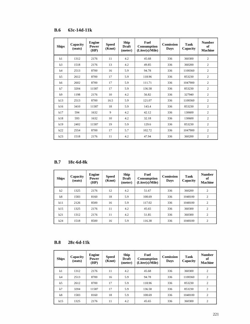
221

B.6 63c-14d-11k

Ships Capacity (seats)

Engine Power (HP)

Speed (Knot)

Ship Draft

(meter)

Fuel Consumption (Liter(s)/Mile)

Comission Days

Tank Capacity

Number of

Machine

k1 1312 2176 11 4.2 45.68 336 360300 2

k3 1518 2176 13 4.2 49.85 336 360200 2

k4 2513 8700 16 5.9 94.78 336 1100360 2

k5 2612 8700 17 5.9 118.96 336 853230 2

k6 2602 8700 17 5.9 111.71 336 1047900 2

k7 3204 11587 17 5.9 136.58 336 853230 2

k9 1198 2176 10 4.2 56.82 336 327940 2

k13 2513 8700 16.5 5.9 121.07 336 1100360 2

k16 3410 11587 18 5.9 143.4 336 853230 2

k17 594 1632 9 4.2 42.12 336 130600 2

k18 593 1632 10 4.2 32.18 336 130600 2

k19 2402 11587 19 5.9 129.6 336 853230 2

k22 2554 8700 17 5.7 102.72 336 1047900 2

k23 1518 2176 11 4.2 47.94 336 360200 2

B.7 18c-6d-8k

Ships Capacity (seats)

Engine Power (HP)

Speed (Knot)

Ship Draft

(meter)

Fuel Consumption (Liter(s)/Mile)

Comission Days

Tank Capacity

Number of

Machine

k2 1325 2176 12 4.2 51.67 336 360200 2

k8 1583 8160 18 5.9 108.69 336 1048100 2

k11 2126 8500 16 5.9 117.02 336 1048100 2

k15 1325 2176 11 4.2 45.65 336 360300 2

k21 1312 2176 11 4.2 51.85 336 360300 2

k24 1518 8500 16 5.9 116.38 336 1048100 2

B.8 28c-6d-11k

Ships Capacity (seats)

Engine Power (HP)

Speed (Knot)

Ship Draft

(meter)

Fuel Consumption (Liter(s)/Mile)

Comission Days

Tank Capacity

Number of

Machine

k1 1312 2176 11 4.2 45.68 336 360300 2

k4 2513 8700 16 5.9 94.78 336 1100360 2

k5 2612 8700 17 5.9 118.96 336 853230 2

k7 3204 11587 17 5.9 136.58 336 853230 2

k8 1583 8160 18 5.9 108.69 336 1048100 2

k15 1325 2176 11 4.2 45.65 336 360300 2

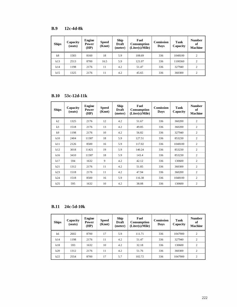
222

B.9 12c-4d-8k

Ships Capacity (seats)

Engine Power (HP)

Speed (Knot)

Ship Draft

(meter)

Fuel Consumption (Liter(s)/Mile)

Comission Days

Tank Capacity

Number of

Machine

k8 1583 8160 18 5.9 108.69 336 1048100 2

k13 2513 8700 16.5 5.9 121.07 336 1100360 2

k14 1198 2176 11 4.2 51.47 336 327940 2

k15 1325 2176 11 4.2 45.65 336 360300 2

B.10 53c-12d-11k

Ships Capacity (seats)

Engine Power (HP)

Speed (Knot)

Ship Draft

(meter)

Fuel Consumption (Liter(s)/Mile)

Comission Days

Tank Capacity

Number of

Machine

k2 1325 2176 12 4.2 51.67 336 360200 2

k3 1518 2176 13 4.2 49.85 336 360200 2

k9 1198 2176 10 4.2 56.82 336 327940 2

k10 2404 11587 18 5.9 127.51 336 853230 2

k11 2126 8500 16 5.9 117.02 336 1048100 2

k12 3018 11421 19 5.9 140.24 336 853230 2

k16 3410 11587 18 5.9 143.4 336 853230 2

k17 594 1632 9 4.2 42.12 336 130600 2

k21 1312 2176 11 4.2 51.85 336 360300 2

k23 1518 2176 11 4.2 47.94 336 360200 2

k24 1518 8500 16 5.9 116.38 336 1048100 2

k25 595 1632 10 4.2 38.08 336 130600 2

B.11 24c-5d-10k

Ships Capacity (seats)

Engine Power (HP)

Speed (Knot)

Ship Draft

(meter)

Fuel Consumption (Liter(s)/Mile)

Comission Days

Tank Capacity

Number of

Machine

k6 2602 8700 17 5.9 111.71 336 1047900 2

k14 1198 2176 11 4.2 51.47 336 327940 2

k18 593 1632 10 4.2 32.18 336 130600 2

k20 1312 2176 11 4.2 51.76 336 360300 2

k22 2554 8700 17 5.7 102.72 336 1047900 2

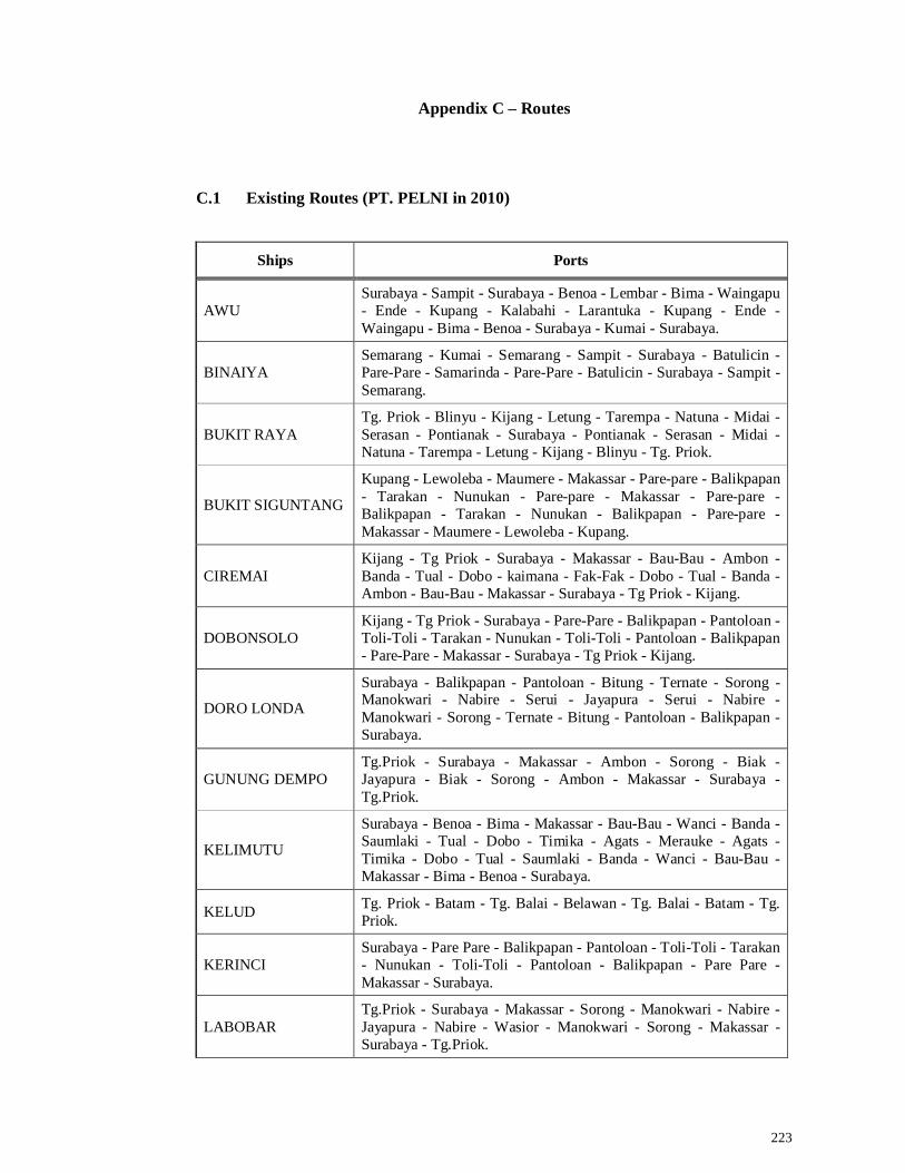
223

Appendix C – Routes

C.1 Existing Routes (PT. PELNI in 2010)

Ships Ports

AWU Surabaya - Sampit - Surabaya - Benoa - Lembar - Bima - Waingapu - Ende - Kupang - Kalabahi - Larantuka - Kupang - Ende - Waingapu - Bima - Benoa - Surabaya - Kumai - Surabaya.

BINAIYA Semarang - Kumai - Semarang - Sampit - Surabaya - Batulicin - Pare-Pare - Samarinda - Pare-Pare - Batulicin - Surabaya - Sampit - Semarang.

BUKIT RAYA Tg. Priok - Blinyu - Kijang - Letung - Tarempa - Natuna - Midai - Serasan - Pontianak - Surabaya - Pontianak - Serasan - Midai - Natuna - Tarempa - Letung - Kijang - Blinyu - Tg. Priok.

BUKIT SIGUNTANG

Kupang - Lewoleba - Maumere - Makassar - Pare-pare - Balikpapan - Tarakan - Nunukan - Pare-pare - Makassar - Pare-pare - Balikpapan - Tarakan - Nunukan - Balikpapan - Pare-pare - Makassar - Maumere - Lewoleba - Kupang.

CIREMAI Kijang - Tg Priok - Surabaya - Makassar - Bau-Bau - Ambon - Banda - Tual - Dobo - kaimana - Fak-Fak - Dobo - Tual - Banda - Ambon - Bau-Bau - Makassar - Surabaya - Tg Priok - Kijang.

DOBONSOLO Kijang - Tg Priok - Surabaya - Pare-Pare - Balikpapan - Pantoloan - Toli-Toli - Tarakan - Nunukan - Toli-Toli - Pantoloan - Balikpapan - Pare-Pare - Makassar - Surabaya - Tg Priok - Kijang.

DORO LONDA

Surabaya - Balikpapan - Pantoloan - Bitung - Ternate - Sorong - Manokwari - Nabire - Serui - Jayapura - Serui - Nabire - Manokwari - Sorong - Ternate - Bitung - Pantoloan - Balikpapan - Surabaya.

GUNUNG DEMPO Tg.Priok - Surabaya - Makassar - Ambon - Sorong - Biak - Jayapura - Biak - Sorong - Ambon - Makassar - Surabaya - Tg.Priok.

KELIMUTU

Surabaya - Benoa - Bima - Makassar - Bau-Bau - Wanci - Banda - Saumlaki - Tual - Dobo - Timika - Agats - Merauke - Agats - Timika - Dobo - Tual - Saumlaki - Banda - Wanci - Bau-Bau - Makassar - Bima - Benoa - Surabaya.

KELUD Tg. Priok - Batam - Tg. Balai - Belawan - Tg. Balai - Batam - Tg. Priok.

KERINCI Surabaya - Pare Pare - Balikpapan - Pantoloan - Toli-Toli - Tarakan - Nunukan - Toli-Toli - Pantoloan - Balikpapan - Pare Pare - Makassar - Surabaya.

LABOBAR Tg.Priok - Surabaya - Makassar - Sorong - Manokwari - Nabire - Jayapura - Nabire - Wasior - Manokwari - Sorong - Makassar - Surabaya - Tg.Priok.

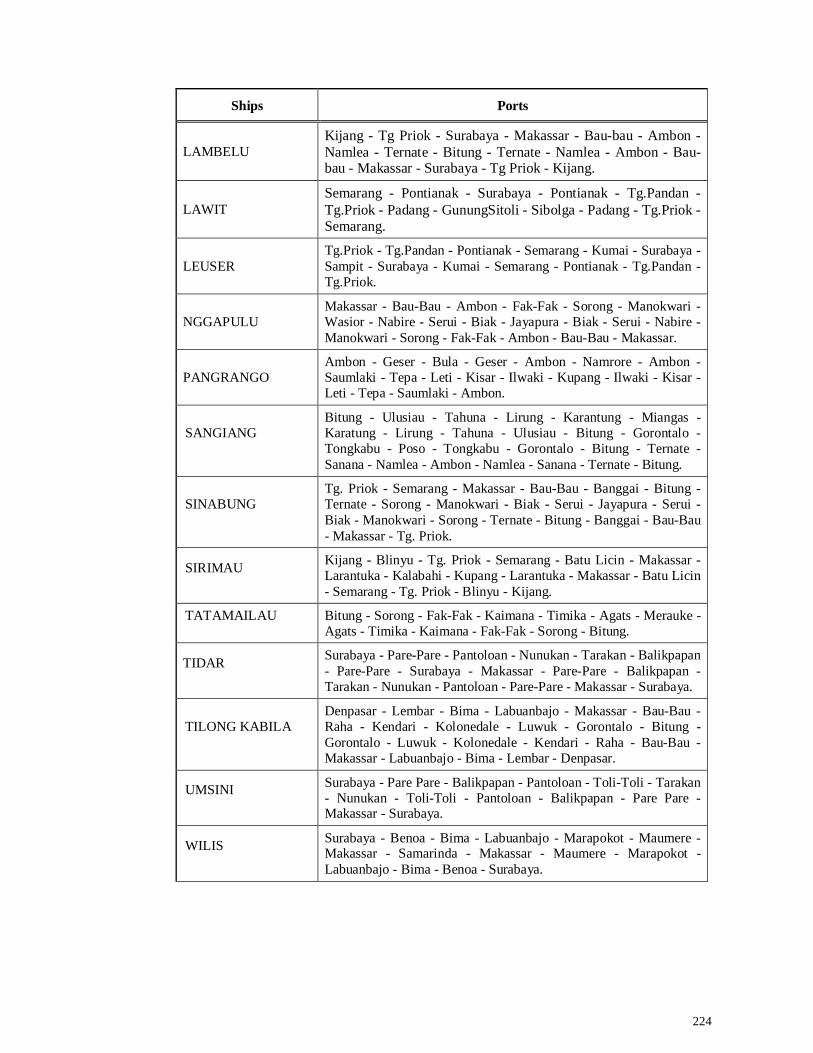
224

Ships Ports

LAMBELU Kijang - Tg Priok - Surabaya - Makassar - Bau-bau - Ambon - Namlea - Ternate - Bitung - Ternate - Namlea - Ambon - Bau-bau - Makassar - Surabaya - Tg Priok - Kijang.

LAWIT Semarang - Pontianak - Surabaya - Pontianak - Tg.Pandan - Tg.Priok - Padang - GunungSitoli - Sibolga - Padang - Tg.Priok - Semarang.

LEUSER Tg.Priok - Tg.Pandan - Pontianak - Semarang - Kumai - Surabaya - Sampit - Surabaya - Kumai - Semarang - Pontianak - Tg.Pandan - Tg.Priok.

NGGAPULU Makassar - Bau-Bau - Ambon - Fak-Fak - Sorong - Manokwari - Wasior - Nabire - Serui - Biak - Jayapura - Biak - Serui - Nabire - Manokwari - Sorong - Fak-Fak - Ambon - Bau-Bau - Makassar.

PANGRANGO Ambon - Geser - Bula - Geser - Ambon - Namrore - Ambon - Saumlaki - Tepa - Leti - Kisar - Ilwaki - Kupang - Ilwaki - Kisar - Leti - Tepa - Saumlaki - Ambon.

SANGIANG

Bitung - Ulusiau - Tahuna - Lirung - Karantung - Miangas - Karatung - Lirung - Tahuna - Ulusiau - Bitung - Gorontalo - Tongkabu - Poso - Tongkabu - Gorontalo - Bitung - Ternate - Sanana - Namlea - Ambon - Namlea - Sanana - Ternate - Bitung.

SINABUNG

Tg. Priok - Semarang - Makassar - Bau-Bau - Banggai - Bitung - Ternate - Sorong - Manokwari - Biak - Serui - Jayapura - Serui - Biak - Manokwari - Sorong - Ternate - Bitung - Banggai - Bau-Bau - Makassar - Tg. Priok.

SIRIMAU

Kijang - Blinyu - Tg. Priok - Semarang - Batu Licin - Makassar - Larantuka - Kalabahi - Kupang - Larantuka - Makassar - Batu Licin - Semarang - Tg. Priok - Blinyu - Kijang.

TATAMAILAU

Bitung - Sorong - Fak-Fak - Kaimana - Timika - Agats - Merauke - Agats - Timika - Kaimana - Fak-Fak - Sorong - Bitung.

TIDAR

Surabaya - Pare-Pare - Pantoloan - Nunukan - Tarakan - Balikpapan - Pare-Pare - Surabaya - Makassar - Pare-Pare - Balikpapan - Tarakan - Nunukan - Pantoloan - Pare-Pare - Makassar - Surabaya.

TILONG KABILA

Denpasar - Lembar - Bima - Labuanbajo - Makassar - Bau-Bau - Raha - Kendari - Kolonedale - Luwuk - Gorontalo - Bitung - Gorontalo - Luwuk - Kolonedale - Kendari - Raha - Bau-Bau - Makassar - Labuanbajo - Bima - Lembar - Denpasar.

UMSINI

Surabaya - Pare Pare - Balikpapan - Pantoloan - Toli-Toli - Tarakan - Nunukan - Toli-Toli - Pantoloan - Balikpapan - Pare Pare - Makassar - Surabaya.

WILIS

Surabaya - Benoa - Bima - Labuanbajo - Marapokot - Maumere - Makassar - Samarinda - Makassar - Maumere - Marapokot - Labuanbajo - Bima - Benoa - Surabaya.

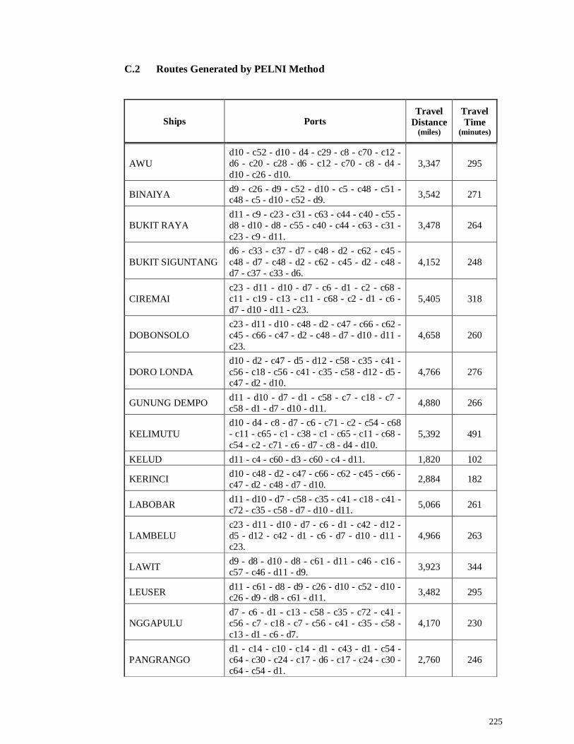
225

C.2 Routes Generated by PELNI Method

Ships Ports Travel

Distance (miles)

Travel Time

(minutes)

AWU d10 - c52 - d10 - d4 - c29 - c8 - c70 - c12 - d6 - c20 - c28 - d6 - c12 - c70 - c8 - d4 - d10 - c26 - d10.

3,347 295

BINAIYA d9 - c26 - d9 - c52 - d10 - c5 - c48 - c51 - c48 - c5 - d10 - c52 - d9. 3,542 271

BUKIT RAYA d11 - c9 - c23 - c31 - c63 - c44 - c40 - c55 - d8 - d10 - d8 - c55 - c40 - c44 - c63 - c31 - c23 - c9 - d11.

3,478 264

BUKIT SIGUNTANG d6 - c33 - c37 - d7 - c48 - d2 - c62 - c45 - c48 - d7 - c48 - d2 - c62 - c45 - d2 - c48 - d7 - c37 - c33 - d6.

4,152 248

CIREMAI c23 - d11 - d10 - d7 - c6 - d1 - c2 - c68 - c11 - c19 - c13 - c11 - c68 - c2 - d1 - c6 - d7 - d10 - d11 - c23.

5,405 318

DOBONSOLO c23 - d11 - d10 - c48 - d2 - c47 - c66 - c62 - c45 - c66 - c47 - d2 - c48 - d7 - d10 - d11 - c23.

4,658 260

DORO LONDA d10 - d2 - c47 - d5 - d12 - c58 - c35 - c41 - c56 - c18 - c56 - c41 - c35 - c58 - d12 - d5 - c47 - d2 - d10.

4,766 276

GUNUNG DEMPO d11 - d10 - d7 - d1 - c58 - c7 - c18 - c7 - c58 - d1 - d7 - d10 - d11. 4,880 266

KELIMUTU d10 - d4 - c8 - d7 - c6 - c71 - c2 - c54 - c68 - c11 - c65 - c1 - c38 - c1 - c65 - c11 - c68 - c54 - c2 - c71 - c6 - d7 - c8 - d4 - d10.

5,392 491

KELUD d11 - c4 - c60 - d3 - c60 - c4 - d11. 1,820 102

KERINCI d10 - c48 - d2 - c47 - c66 - c62 - c45 - c66 - c47 - d2 - c48 - d7 - d10. 2,884 182

LABOBAR d11 - d10 - d7 - c58 - c35 - c41 - c18 - c41 - c72 - c35 - c58 - d7 - d10 - d11. 5,066 261

LAMBELU c23 - d11 - d10 - d7 - c6 - d1 - c42 - d12 - d5 - d12 - c42 - d1 - c6 - d7 - d10 - d11 - c23.

4,966 263

LAWIT d9 - d8 - d10 - d8 - c61 - d11 - c46 - c16 - c57 - c46 - d11 - d9. 3,923 344

LEUSER d11 - c61 - d8 - d9 - c26 - d10 - c52 - d10 - c26 - d9 - d8 - c61 - d11. 3,482 295

NGGAPULU d7 - c6 - d1 - c13 - c58 - c35 - c72 - c41 - c56 - c7 - c18 - c7 - c56 - c41 - c35 - c58 - c13 - d1 - c6 - d7.

4,170 230

PANGRANGO d1 - c14 - c10 - c14 - d1 - c43 - d1 - c54 - c64 - c30 - c24 - c17 - d6 - c17 - c24 - c30 - c64 - c54 - d1.

2,760 246

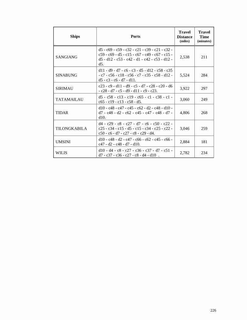
226

Ships Ports Travel

Distance (miles)

Travel Time

(minutes)

SANGIANG

d5 - c69 - c59 - c32 - c21 - c39 - c21 - c32 - c59 - c69 - d5 - c15 - c67 - c49 - c67 - c15 - d5 - d12 - c53 - c42 - d1 - c42 - c53 - d12 - d5.

2,538 211

SINABUNG d11 - d9 - d7 - c6 - c3 - d5 - d12 - c58 - c35 - c7 - c56 - c18 - c56 - c7 - c35 - c58 - d12 - d5 - c3 - c6 - d7 - d11.

5,524 284

SIRIMAU c23 - c9 - d11 - d9 - c5 - d7 - c28 - c20 - d6 - c28 - d7 - c5 - d9 - d11 - c9 - c23. 3,922 297

TATAMAILAU d5 - c58 - c13 - c19 - c65 - c1 - c38 - c1 - c65 - c19 - c13 - c58 - d5. 3,060 249

TIDAR d10 - c48 - c47 - c45 - c62 - d2 - c48 - d10 - d7 - c48 - d2 - c62 - c45 - c47 - c48 - d7 - d10.

4,806 268

TILONGKABILA d4 - c29 - c8 - c27 - d7 - c6 - c50 - c22 - c25 - c34 - c15 - d5 - c15 - c34 - c25 - c22 - c50 - c6 - d7 - c27 - c8 - c29 - d4.

3,046 259

UMSINI d10 - c48 - d2 - c47 - c66 - c62 - c45 - c66 - c47 - d2 - c48 - d7 - d10. 2,884 181

WILIS d10 - d4 - c8 - c27 - c36 - c37 - d7 - c51 - d7 - c37 - c36 - c27 - c8 - d4 - d10 . 2,782 234

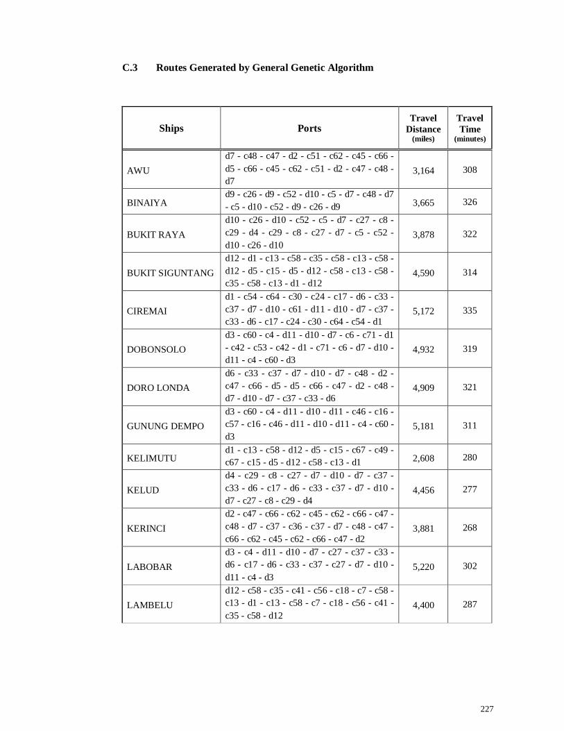
227

C.3 Routes Generated by General Genetic Algorithm

Ships Ports Travel

Distance (miles)

Travel Time

(minutes)

AWU d7 - c48 - c47 - d2 - c51 - c62 - c45 - c66 - d5 - c66 - c45 - c62 - c51 - d2 - c47 - c48 - d7

3,164 308

BINAIYA d9 - c26 - d9 - c52 - d10 - c5 - d7 - c48 - d7 - c5 - d10 - c52 - d9 - c26 - d9 3,665 326

BUKIT RAYA d10 - c26 - d10 - c52 - c5 - d7 - c27 - c8 - c29 - d4 - c29 - c8 - c27 - d7 - c5 - c52 - d10 - c26 - d10

3,878 322

BUKIT SIGUNTANG d12 - d1 - c13 - c58 - c35 - c58 - c13 - c58 - d12 - d5 - c15 - d5 - d12 - c58 - c13 - c58 - c35 - c58 - c13 - d1 - d12

4,590 314

CIREMAI d1 - c54 - c64 - c30 - c24 - c17 - d6 - c33 - c37 - d7 - d10 - c61 - d11 - d10 - d7 - c37 - c33 - d6 - c17 - c24 - c30 - c64 - c54 - d1

5,172 335

DOBONSOLO d3 - c60 - c4 - d11 - d10 - d7 - c6 - c71 - d1 - c42 - c53 - c42 - d1 - c71 - c6 - d7 - d10 - d11 - c4 - c60 - d3

4,932 319

DORO LONDA d6 - c33 - c37 - d7 - d10 - d7 - c48 - d2 - c47 - c66 - d5 - d5 - c66 - c47 - d2 - c48 - d7 - d10 - d7 - c37 - c33 - d6

4,909 321

GUNUNG DEMPO d3 - c60 - c4 - d11 - d10 - d11 - c46 - c16 - c57 - c16 - c46 - d11 - d10 - d11 - c4 - c60 - d3

5,181 311

KELIMUTU d1 - c13 - c58 - d12 - d5 - c15 - c67 - c49 - c67 - c15 - d5 - d12 - c58 - c13 - d1 2,608 280

KELUD d4 - c29 - c8 - c27 - d7 - d10 - d7 - c37 - c33 - d6 - c17 - d6 - c33 - c37 - d7 - d10 - d7 - c27 - c8 - c29 - d4

4,456 277

KERINCI d2 - c47 - c66 - c62 - c45 - c62 - c66 - c47 - c48 - d7 - c37 - c36 - c37 - d7 - c48 - c47 - c66 - c62 - c45 - c62 - c66 - c47 - d2

3,881 268

LABOBAR d3 - c4 - d11 - d10 - d7 - c27 - c37 - c33 - d6 - c17 - d6 - c33 - c37 - c27 - d7 - d10 - d11 - c4 - d3

5,220 302

LAMBELU d12 - c58 - c35 - c41 - c56 - c18 - c7 - c58 - c13 - d1 - c13 - c58 - c7 - c18 - c56 - c41 - c35 - c58 - d12

4,400 287

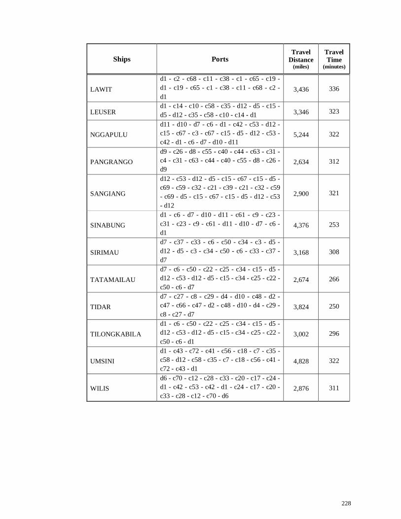
228

Ships Ports Travel

Distance (miles)

Travel Time

(minutes)

LAWIT d1 - c2 - c68 - c11 - c38 - c1 - c65 - c19 - d1 - c19 - c65 - c1 - c38 - c11 - c68 - c2 - d1

3,436 336

LEUSER d1 - c14 - c10 - c58 - c35 - d12 - d5 - c15 - d5 - d12 - c35 - c58 - c10 - c14 - d1 3,346 323

NGGAPULU d11 - d10 - d7 - c6 - d1 - c42 - c53 - d12 - c15 - c67 - c3 - c67 - c15 - d5 - d12 - c53 - c42 - d1 - c6 - d7 - d10 - d11

5,244 322

PANGRANGO d9 - c26 - d8 - c55 - c40 - c44 - c63 - c31 - c4 - c31 - c63 - c44 - c40 - c55 - d8 - c26 - d9

2,634 312

SANGIANG

d12 - c53 - d12 - d5 - c15 - c67 - c15 - d5 - c69 - c59 - c32 - c21 - c39 - c21 - c32 - c59 - c69 - d5 - c15 - c67 - c15 - d5 - d12 - c53 - d12

2,900 321

SINABUNG d1 - c6 - d7 - d10 - d11 - c61 - c9 - c23 - c31 - c23 - c9 - c61 - d11 - d10 - d7 - c6 - d1

4,376 253

SIRIMAU d7 - c37 - c33 - c6 - c50 - c34 - c3 - d5 - d12 - d5 - c3 - c34 - c50 - c6 - c33 - c37 - d7

3,168 308

TATAMAILAU d7 - c6 - c50 - c22 - c25 - c34 - c15 - d5 - d12 - c53 - d12 - d5 - c15 - c34 - c25 - c22 - c50 - c6 - d7

2,674 266

TIDAR d7 - c27 - c8 - c29 - d4 - d10 - c48 - d2 - c47 - c66 - c47 - d2 - c48 - d10 - d4 - c29 - c8 - c27 - d7

3,824 250

TILONGKABILA d1 - c6 - c50 - c22 - c25 - c34 - c15 - d5 - d12 - c53 - d12 - d5 - c15 - c34 - c25 - c22 - c50 - c6 - d1

3,002 296

UMSINI d1 - c43 - c72 - c41 - c56 - c18 - c7 - c35 - c58 - d12 - c58 - c35 - c7 - c18 - c56 - c41 - c72 - c43 - d1

4,828 322

WILIS d6 - c70 - c12 - c28 - c33 - c20 - c17 - c24 - d1 - c42 - c53 - c42 - d1 - c24 - c17 - c20 - c33 - c28 - c12 - c70 - d6

2,876 311

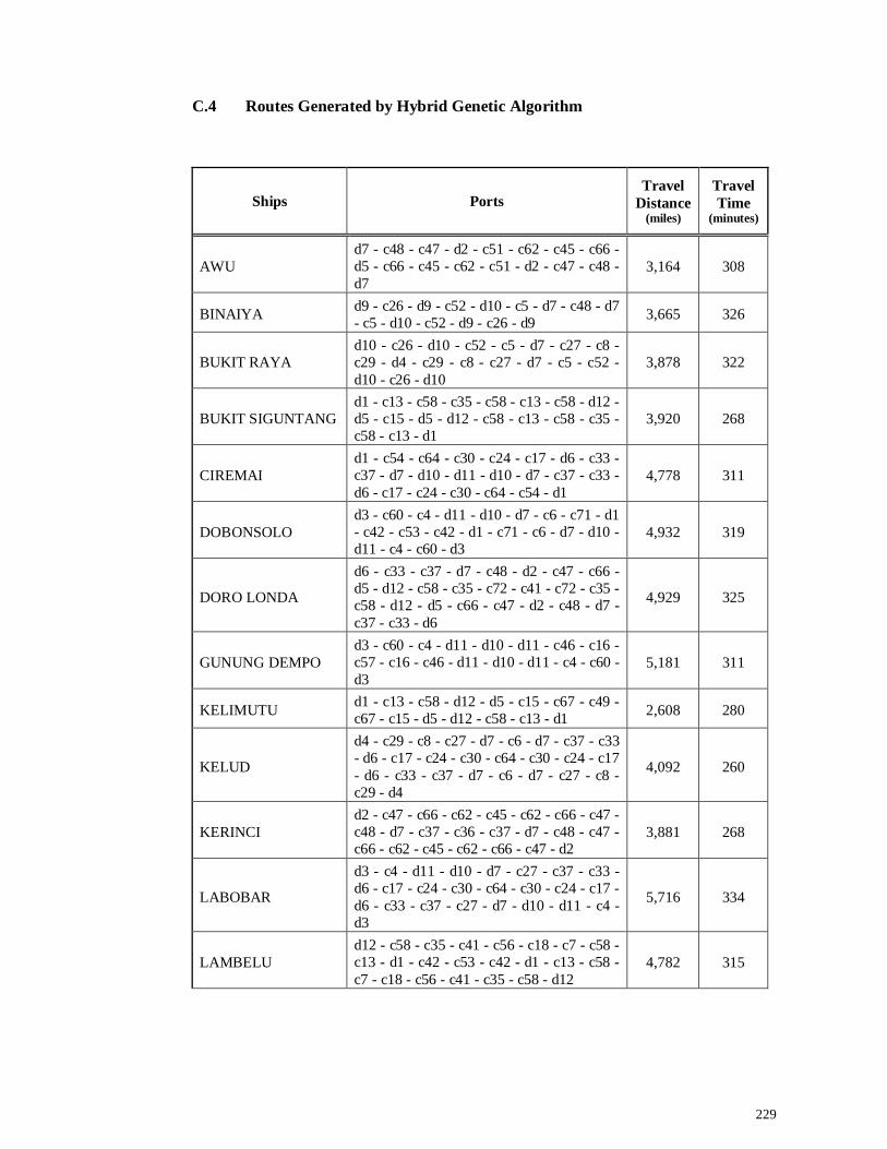
229

C.4 Routes Generated by Hybrid Genetic Algorithm

Ships Ports Travel

Distance (miles)

Travel Time

(minutes)

AWU d7 - c48 - c47 - d2 - c51 - c62 - c45 - c66 - d5 - c66 - c45 - c62 - c51 - d2 - c47 - c48 - d7

3,164 308

BINAIYA d9 - c26 - d9 - c52 - d10 - c5 - d7 - c48 - d7 - c5 - d10 - c52 - d9 - c26 - d9 3,665 326

BUKIT RAYA d10 - c26 - d10 - c52 - c5 - d7 - c27 - c8 - c29 - d4 - c29 - c8 - c27 - d7 - c5 - c52 - d10 - c26 - d10

3,878 322

BUKIT SIGUNTANG d1 - c13 - c58 - c35 - c58 - c13 - c58 - d12 - d5 - c15 - d5 - d12 - c58 - c13 - c58 - c35 - c58 - c13 - d1

3,920 268

CIREMAI d1 - c54 - c64 - c30 - c24 - c17 - d6 - c33 - c37 - d7 - d10 - d11 - d10 - d7 - c37 - c33 - d6 - c17 - c24 - c30 - c64 - c54 - d1

4,778 311

DOBONSOLO d3 - c60 - c4 - d11 - d10 - d7 - c6 - c71 - d1 - c42 - c53 - c42 - d1 - c71 - c6 - d7 - d10 - d11 - c4 - c60 - d3

4,932 319

DORO LONDA

d6 - c33 - c37 - d7 - c48 - d2 - c47 - c66 - d5 - d12 - c58 - c35 - c72 - c41 - c72 - c35 - c58 - d12 - d5 - c66 - c47 - d2 - c48 - d7 - c37 - c33 - d6

4,929 325

GUNUNG DEMPO d3 - c60 - c4 - d11 - d10 - d11 - c46 - c16 - c57 - c16 - c46 - d11 - d10 - d11 - c4 - c60 - d3

5,181 311

KELIMUTU d1 - c13 - c58 - d12 - d5 - c15 - c67 - c49 - c67 - c15 - d5 - d12 - c58 - c13 - d1 2,608 280

KELUD

d4 - c29 - c8 - c27 - d7 - c6 - d7 - c37 - c33 - d6 - c17 - c24 - c30 - c64 - c30 - c24 - c17 - d6 - c33 - c37 - d7 - c6 - d7 - c27 - c8 - c29 - d4

4,092 260

KERINCI d2 - c47 - c66 - c62 - c45 - c62 - c66 - c47 - c48 - d7 - c37 - c36 - c37 - d7 - c48 - c47 - c66 - c62 - c45 - c62 - c66 - c47 - d2

3,881 268

LABOBAR

d3 - c4 - d11 - d10 - d7 - c27 - c37 - c33 - d6 - c17 - c24 - c30 - c64 - c30 - c24 - c17 - d6 - c33 - c37 - c27 - d7 - d10 - d11 - c4 - d3

5,716 334

LAMBELU d12 - c58 - c35 - c41 - c56 - c18 - c7 - c58 - c13 - d1 - c42 - c53 - c42 - d1 - c13 - c58 - c7 - c18 - c56 - c41 - c35 - c58 - d12

4,782 315

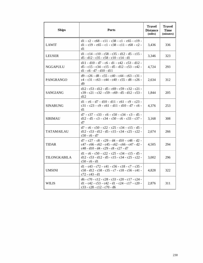
230

Ships Ports Travel

Distance (miles)

Travel Time

(minutes)

LAWIT d1 - c2 - c68 - c11 - c38 - c1 - c65 - c19 - d1 - c19 - c65 - c1 - c38 - c11 - c68 - c2 - d1

3,436 336

LEUSER d1 - c14 - c10 - c58 - c35 - d12 - d5 - c15 - d5 - d12 - c35 - c58 - c10 - c14 - d1 3,346 323

NGGAPULU d11 - d10 - d7 - c6 - d1 - c42 - c53 - d12 - d5 - c15 - c34 - c15 - d5 - d12 - c53 - c42 - d1 - c6 - d7 - d10 - d11

4,724 293

PANGRANGO d9 - c26 - d8 - c55 - c40 - c44 - c63 - c31 - c4 - c31 - c63 - c44 - c40 - c55 - d8 - c26 - d9

2,634 312

SANGIANG d12 - c53 - d12 - d5 - c69 - c59 - c32 - c21 - c39 - c21 - c32 - c59 - c69 - d5 - d12 - c53 - d12

1,844 205

SINABUNG d1 - c6 - d7 - d10 - d11 - c61 - c9 - c23 - c31 - c23 - c9 - c61 - d11 - d10 - d7 - c6 - d1

4,376 253

SIRIMAU d7 - c37 - c33 - c6 - c50 - c34 - c3 - d5 - d12 - d5 - c3 - c34 - c50 - c6 - c33 - c37 - d7

3,168 308

TATAMAILAU d7 - c6 - c50 - c22 - c25 - c34 - c15 - d5 - d12 - c53 - d12 - d5 - c15 - c34 - c25 - c22 - c50 - c6 - d7

2,674 266

TIDAR d7 - c27 - c8 - c29 - d4 - d10 - c48 - d2 - c47 - c66 - c62 - c45 - c62 - c66 - c47 - d2 - c48 - d10 - d4 - c29 - c8 - c27 - d7

4,505 294

TILONGKABILA d1 - c6 - c50 - c22 - c25 - c34 - c15 - d5 - d12 - c53 - d12 - d5 - c15 - c34 - c25 - c22 - c50 - c6 - d1

3,002 296

UMSINI d1 - c43 - c72 - c41 - c56 - c18 - c7 - c35 - c58 - d12 - c58 - c35 - c7 - c18 - c56 - c41 - c72 - c43 - d1

4,828 322

WILIS d6 - c70 - c12 - c28 - c33 - c20 - c17 - c24 - d1 - c42 - c53 - c42 - d1 - c24 - c17 - c20 - c33 - c28 - c12 - c70 - d6

2,876 311

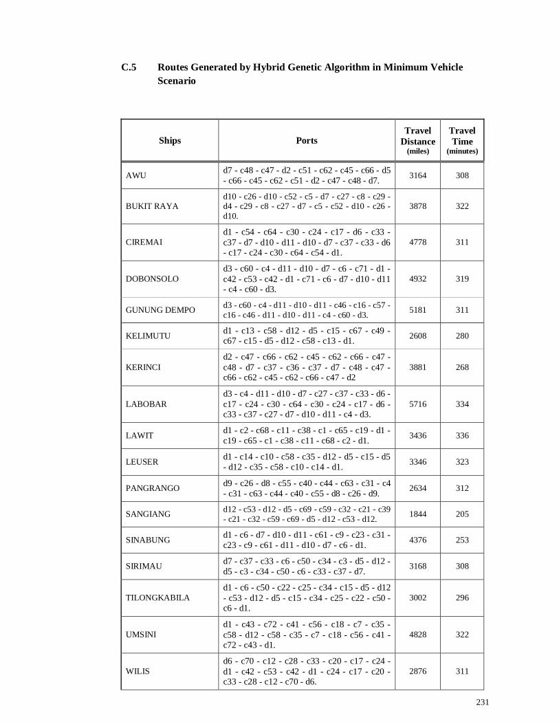
231

C.5 Routes Generated by Hybrid Genetic Algorithm in Minimum Vehicle Scenario

Ships Ports Travel

Distance (miles)

Travel Time

(minutes)

AWU d7 - c48 - c47 - d2 - c51 - c62 - c45 - c66 - d5 - c66 - c45 - c62 - c51 - d2 - c47 - c48 - d7. 3164 308

BUKIT RAYA d10 - c26 - d10 - c52 - c5 - d7 - c27 - c8 - c29 - d4 - c29 - c8 - c27 - d7 - c5 - c52 - d10 - c26 - d10.

3878 322

CIREMAI d1 - c54 - c64 - c30 - c24 - c17 - d6 - c33 - c37 - d7 - d10 - d11 - d10 - d7 - c37 - c33 - d6 - c17 - c24 - c30 - c64 - c54 - d1.

4778 311

DOBONSOLO d3 - c60 - c4 - d11 - d10 - d7 - c6 - c71 - d1 - c42 - c53 - c42 - d1 - c71 - c6 - d7 - d10 - d11 - c4 - c60 - d3.

4932 319

GUNUNG DEMPO d3 - c60 - c4 - d11 - d10 - d11 - c46 - c16 - c57 - c16 - c46 - d11 - d10 - d11 - c4 - c60 - d3. 5181 311

KELIMUTU d1 - c13 - c58 - d12 - d5 - c15 - c67 - c49 - c67 - c15 - d5 - d12 - c58 - c13 - d1. 2608 280

KERINCI d2 - c47 - c66 - c62 - c45 - c62 - c66 - c47 - c48 - d7 - c37 - c36 - c37 - d7 - c48 - c47 - c66 - c62 - c45 - c62 - c66 - c47 - d2

3881 268

LABOBAR d3 - c4 - d11 - d10 - d7 - c27 - c37 - c33 - d6 - c17 - c24 - c30 - c64 - c30 - c24 - c17 - d6 - c33 - c37 - c27 - d7 - d10 - d11 - c4 - d3.

5716 334

LAWIT d1 - c2 - c68 - c11 - c38 - c1 - c65 - c19 - d1 - c19 - c65 - c1 - c38 - c11 - c68 - c2 - d1. 3436 336

LEUSER d1 - c14 - c10 - c58 - c35 - d12 - d5 - c15 - d5 - d12 - c35 - c58 - c10 - c14 - d1. 3346 323

PANGRANGO d9 - c26 - d8 - c55 - c40 - c44 - c63 - c31 - c4 - c31 - c63 - c44 - c40 - c55 - d8 - c26 - d9. 2634 312

SANGIANG d12 - c53 - d12 - d5 - c69 - c59 - c32 - c21 - c39 - c21 - c32 - c59 - c69 - d5 - d12 - c53 - d12. 1844 205

SINABUNG d1 - c6 - d7 - d10 - d11 - c61 - c9 - c23 - c31 - c23 - c9 - c61 - d11 - d10 - d7 - c6 - d1. 4376 253

SIRIMAU d7 - c37 - c33 - c6 - c50 - c34 - c3 - d5 - d12 - d5 - c3 - c34 - c50 - c6 - c33 - c37 - d7. 3168 308

TILONGKABILA d1 - c6 - c50 - c22 - c25 - c34 - c15 - d5 - d12 - c53 - d12 - d5 - c15 - c34 - c25 - c22 - c50 - c6 - d1.

3002 296

UMSINI d1 - c43 - c72 - c41 - c56 - c18 - c7 - c35 - c58 - d12 - c58 - c35 - c7 - c18 - c56 - c41 - c72 - c43 - d1.

4828 322

WILIS d6 - c70 - c12 - c28 - c33 - c20 - c17 - c24 - d1 - c42 - c53 - c42 - d1 - c24 - c17 - c20 - c33 - c28 - c12 - c70 - d6.

2876 311

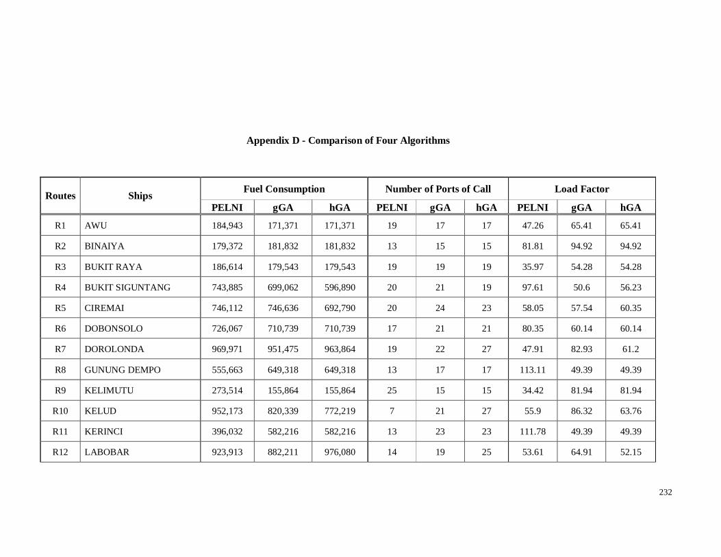
232

Appendix D - Comparison of Four Algorithms

Routes Ships Fuel Consumption Number of Ports of Call Load Factor

PELNI gGA hGA PELNI gGA hGA PELNI gGA hGA

R1 AWU 184,943 171,371 171,371 19 17 17 47.26 65.41 65.41

R2 BINAIYA 179,372 181,832 181,832 13 15 15 81.81 94.92 94.92

R3 BUKIT RAYA 186,614 179,543 179,543 19 19 19 35.97 54.28 54.28

R4 BUKIT SIGUNTANG 743,885 699,062 596,890 20 21 19 97.61 50.6 56.23

R5 CIREMAI 746,112 746,636 692,790 20 24 23 58.05 57.54 60.35

R6 DOBONSOLO 726,067 710,739 710,739 17 21 21 80.35 60.14 60.14

R7 DOROLONDA 969,971 951,475 963,864 19 22 27 47.91 82.93 61.2

R8 GUNUNG DEMPO 555,663 649,318 649,318 13 17 17 113.11 49.39 49.39

R9 KELIMUTU 273,514 155,864 155,864 25 15 15 34.42 81.94 81.94

R10 KELUD 952,173 820,339 772,219 7 21 27 55.9 86.32 63.76

R11 KERINCI 396,032 582,216 582,216 13 23 23 111.78 49.39 49.39

R12 LABOBAR 923,913 882,211 976,080 14 19 25 53.61 64.91 52.15