joint modelling of extreme ocean environments …joint modelling of extreme ocean environments...
TRANSCRIPT
Joint modelling of extreme ocean environments incorporating covariate effects
Philip Jonathan
Shell Research Ltd., Chester, CH1 3SH, UK.
Kevin Ewans
Sarawak Shell Bhd., 50450 Kuala Lumpur, Malaysia.
David Randell
Shell Research Ltd., Chester, CH1 3SH, UK.
Abstract
Characterising the joint distribution of extremes of ocean environmental variables such as significant wave
height (HS) and spectral peak period (TP ) is important for understanding extreme ocean environments
and in the design and assessment of marine and coastal structures. Many applications of multivariate
extreme value analysis adopt models that assume a particular form of extremal dependence between vari-
ables without justification. Models are also typically restricted to joint regions in which all variables are
extreme, but regions where only a subset of variables are extreme can be equally important for design.
The conditional extremes model of Heffernan and Tawn (2004) provides one approach to overcoming these
difficulties.
Here, we extend the conditional extremes model to incorporate covariate effects in all of threshold selection,
marginal and dependence modelling. Quantile regression is used to select appropriate covariate-dependent
extreme value thresholds. Marginal and dependence modelling of extremes is performed within a penalised
likelihood framework, using a Fourier parameterisation of marginal and dependence model parameters, with
cross-validation to estimate suitable model parameter roughness, and bootstrapping to estimate parameter
uncertainty with respect to covariate.
1
We illustrate the approach in application to joint modelling of storm peak HS and TP at a Northern North
Sea location with storm direction as covariate. We evaluate the impact of incorporating directional effects
on estimates for return values, including those of a structure variable, similar to the structural response of
a floating structure. We believe the approach offers the ocean engineer a straightforward procedure, based
on sound statistics, to incorporate covariate effects in estimation of joint extreme environmental conditions.
Keywords: offshore design; joint extremes; conditional extremes; covariates;
Preprint submitted to Coastal Engineering 7th May 2013
1. Introduction
It is well known that the characteristics of extreme ocean environments vary with respect to a number
of covariates. For example, extremes of HS vary with wave direction and season (as demonstrated by,
e.g., Ewans and Jonathan (2008) and Jonathan and Ewans (2011)). Incorporation of covariate effects is
important to successful marginal modelling of environmental extremes (see, e.g., Jonathan et al. 2008). It
would seem reasonable, therefore, to expect that covariate effects are important in modelling joint extremes
also in general.
Marginal modelling of extremes with covariates has been performed for many years. Some authors follow
the approach of Davison and Smith (1990), parameterising extreme value model parameters in terms of
one or more covariates (see, e.g., Chavez-Demoulin and Davison 2005). Other authors prefer to transform
(or whiten) the sample to remove the effects of covariates (see Eastoe and Tawn 2009) prior to extreme
value analysis. Marginal (and dependence) modelling of extremes with covariates requires the specification
of a threshold for extreme value modelling. A number of authors (see, e.g., Anderson et al. 2001) have
commented on the importance of specifying a covariate-dependent threshold when covariate effects are
suspected. One approach to covariate-dependent threshold specification is quantile regression (Koenker
2005), illustrated recently in environmental applications by Kysely et al. (2010) and Northrop and Jonathan
(2011).
Characterising the joint distribution of extremes of ocean environmental parameters is important in un-
derstanding extreme ocean environments and in the design and assessment of marine structures. The
conditional extremes model of Heffernan and Tawn (2004) provides a straightforward procedure for mod-
elling multivariate extremal dependence in the absence of covariates. Jonathan et al. (2010) illustrate the
application of conditional extremes model to characterise the dependence structure of storm peak signific-
ant wave height (HS) and wave spectral peak period (TP ) and estimate the return values of TP conditional
on extreme values of HS . To estimate the conditional extremes model for bivariate extremes of random
3
variables X1 (HS , say) and X2 (TP , say), the following procedure is appropriate. (a) Select a range of
appropriate thresholds for threshold exceedance modelling for each variable in turn. (b) Fit marginal gen-
eralised Pareto models to threshold exceedances of the sample data for each variable in turn for different
threshold choices, plot the values of model parameter estimates as a function of threshold, and select the
lowest threshold value per variable corresponding to approximately stable models. (c) Transform X1 and
X2 in turn to Gumbel scale (to X1 and X2) using the probability integral transform. (d) Fit the conditional
extremes model for X2|X1 (and X1|X2) in turn for various choices of threshold of the conditioning variate,
retain the estimated model parameters and residuals, plot the values of model parameter estimates and
examine residuals as a function of threshold, and select the lowest threshold per variable consistent with
modelling assumptions. (e) Simulate joint extremes on the standard Gumbel scale under the model, and
transform realisations to the original scale using the probability integral transform.
To our knowledge, there is no literature on incorporation of covariate effects within the conditional ex-
tremes model, the topic of this article. The layout of the paper is as follows. In section 2, we introduce a
motivating application. Section 3 is a description of the marginal model (incorporating threshold model-
ling, generalised Pareto modelling of threshold exceedances and transformation to Gumbel scale), and the
extended conditional extremes model incorporating covariate effects. Section 4 addresses the estimation of
conditional extremes for the Northern North Sea location under consideration, followed by a more general
discussion and conclusions in section 5.
2. Data
We motivate and illustrate the methodology by considering joint estimation of extreme values of storm
peak HS and TP with directional covariate at a location in the northern North Sea. Data correspond to
hindcast values of storm peak HS over threshold, observed during periods of storm events, and associated
values for TP . The sample consists of 1163 pairs of values for the period October 1964 to August 1998.
4
Figure 1 shows the approximate North Sea location corresponding to the data, and the relatively long
fetches for waves emanating from the Atlantic Ocean, the Norwegian Sea and the North Sea. With
direction from which waves travel expressed in degrees clockwise with respect to north, Figure 2 gives
scatter plots of HS (horizontal) and TP (vertical) for directional sectors corresponding approximately to
those in Figure 1. It can be seen that HS−TP dependence for Atlantic storms (directional sector [230, 280))
is quite different to that for storms emanating from the south (directional sector [140, 200)), suggesting
that the dependence between HS and TP varies as a function of direction, and that this dependence should
be accommodated in any joint modelling of extremes of HS and TP .
[Figure 1 about here.]
[Figure 2 about here.]
3. Model
The application introduced above suggests that we treat storm peak HS and associated TP as varying with
storm direction in order to characterise their joint extremal behaviour. Consider therefore two random
variables X1(θ), X2(θ) of common covariate θ. We are interesting in modelling their joint extremal structure
for any particular value of covariate θ. We assume that the joint tail of X1(θ) and X2(θ) can be characterised
adequately using the single covariate θ.
In this section we describe the extension of the conditional extremes modelling procedure, outlined in
section 1, to incorporate covariates. Sections 3.1 and 3.2 outline the coupled marginal generalised Pareto
modelling of threshold exceedances and quantile regression for threshold selection respectively. Section 3.3
discusses transformation to standard Gumbel scale, necessary for application of the conditional extremes
model in section 3.4. Finally, the adoption of Fourier series representations for model parameter functions
is outlined in section 3.5.
5
3.1. Generalised Pareto model for threshold exceedances
Marginally, for each of X1(θ), X2(θ) in turn for a given value of θ, we assume that, conditional on exceeding
a large value, the corresponding random variables are generalised Pareto distributed:
Pr(Xj(θ) > x|Xj(θ) > ψj(θ; τj∗)) = (1 +ξj(θ)
ζj(θ)(x− ψj(θ; τj∗)))−1/ξj(θ) for j = 1, 2
for x > ψj(θ; τj∗), (1+ξj(θ)ζj(θ)
(x−ψj(θ; τj∗))) > 0 and ζj(θ) > 0. ψj(θ; τj∗) is a pre-selected quantile threshold,
assumed to be a smooth function of θ, associated with a non exceedance probability τj∗:
Pr(Xj(θ) 6 ψj(θ; τj∗)) = τj∗ .
Model parameters ξj(θ), ζj(θ), respectively generalised Pareto shape and scale, are also assumed to be
smooth functions of covariate. For a sample of values {xij}ni=1, j = 1, 2, corresponding to set {θi}ni=1 of
known covariate values, and pre-specified threshold ψj(θ; τj∗), estimates for the values of the functions
ξj(θ) and ζj(θ) at {θi}ni=1 can be obtained in principle by maximum likelihood estimation, by minimising
the negative log-likelihood:
`GP,j =n∑i=1
log ζj(θi) +1
ξj(θi)log(1 +
ξj(θi)
ζj(θi)(xij − ψj(θi; τj∗))) for j = 1, 2 .
Each of the parameter functions ψj(θ; τj∗), ξj(θ) and ζj(θ) can be specified as a linear combination of
suitable basis functions, such as periodic splines and Fourier series for periodic covariates such as direction,
as discussed in section 3.5. In this case, we regulate parameter smoothness with covariate using a penalised
likelihood fitting criterion:
`∗GP,j = `GP,j + λξjRξj + λζjRζj for j = 1, 2
6
for roughness coefficients λξj , λζj , and parameter roughnesses Rξj , Rζj which are easily evaluated (see Sec-
tion 3.5) for suitable choice of basis. The values of roughness coefficients are selected using cross-validation
to maximise the predictive performance of the model. 10-fold cross-validation was used throughout this
work.
3.2. Quantile regression model for thresholds
For each random variable in turn, the quantile threshold ψj(θ; τ) corresponding to quantile probability τ
is estimated using quantile regression, by minimising the roughness penalised loss criterion:
`∗QR,j = {τn∑
i,rij≥0|rij |+ (1− τ)
n∑i,rij<0
|rij |}+ λψjRψj
for j = 1, 2
and residuals rij = xij − ψj(θi; τ). The terms in parentheses correspond to the unpenalised quantile
regression loss criterion. Parameter roughness Rψjcan be evaluated in closed form (see Section 3.5) for
efficient estimation. The value of roughness coefficient λψjis selected using cross-validation to maximise
the predictive performance of the quantile regression model.
In practice, quantile regression thresholds are estimated for an increasing sequence of D quantile probab-
ilities 0 < τ1 < τ2 < ... < τd < ... < τD < 1. For each choice of τd, standard diagnostic plots for generalised
Pareto fitting (such as the variation of the estimated shape parameter or some extreme quantile estimate
with threshold) are examined (see, e.g., Scarrott and MacDonald 2012). The lowest value of quantile
probability consistent with an adequate generalised Pareto fit is selected as τj∗. The quantile regression
threshold estimates for quantile probabilities 6 τj∗ are useful for marginal transformation to standard
Gumbel scale, discussed in the next section.
7
3.3. Marginal transformation to standard Gumbel scale
The conditional extremes model is applied to random variables with standard Gumbel marginal distribu-
tions. For each random variable in turn, the quantile regression models for different quantile probabilities,
and the marginal generalised Pareto model for threshold exceedances, provide a means to transform from
sample {xij}ni=1 corresponding to random variable Xj(θ) at the set {θi}ni=1 of known covariate values to
an equivalent sample {xij}ni=1 corresponding to random variable Xj(θ) with approximately a standard
Gumbel distribution for any θ.
Above the threshold ψj(θ; τj∗), the unconditional cumulative distribution function for threshold exceedances
x > ψj(θ; τj∗), for any value of θ, is given by:
Pr(Xj(θ) 6 x) = 1− (1− τj∗) Pr(Xj(θ) > x|Xj(θ) > ψj(θ; τj∗)) for j = 1, 2 .
Below the threshold, in the absence of a parametric form for the cumulative distribution function, we
approximate it using:
Pr(Xj(θ) 6 x) ≈ τd + (τd − τd−1)(x− ψj(θ; τd−1))
(ψj(θ; τd)− ψj(θ; τd−1))for j = 1, 2
where ψj(θ; τd−1) 6 x < ψj(θ; τd) for the sequence of quantile probabilities τd such that τd 6 τj∗.
Using the probability integral transform, we can transform from original to standard Gumbel scales, since:
Pr(Xj(θ) 6 x) = exp(− exp(−x)) = Pr(Xj(θ) 6 x) for j = 1, 2
so that the individuals in the transformed sample {xij}ni=1, j = 1, 2 are given by:
xij = − log(− log(Pr(Xj(θi) 6 xij))) for i = 1, 2, ..., n, and j = 1, 2
8
now assumed to be marginally stationary.
3.4. Conditional extremes model
For positively dependent random variables X1(θ), X2(θ) with standard Gumbel marginal distributions for
any θ, we extend the asymptotic argument of Heffernan and Tawn (2004) for the form of the conditional
distribution of Xjc(θ), jc = 1, 2 given the value of Xj(θ), j = 1, 2, j 6= jc for any value of covariate θ :
(Xjc(θ)|Xj(θ) = x) = αj(θ)x+ xβj(θ)Wj(θ) for j, jc = 1, 2, jc 6= j
and x > φj(κj∗) where φj(κj∗) is a threshold with non-exceedance probability κj∗ above which the con-
ditional extremes model fits well. The parameter functions αj(θ) ∈ [0, 1], βj(θ) ∈ (−∞, 1] vary smoothly
with covariate θ. Wj(θ) is a random variable drawn from an unknown distribution. We assume that
the standardised variable Zj = (Wj(θ) − µj(θ))/σj(θ) follows a common distribution Gj , independent of
covariate, for smooth location and scale parameter functions µj(θ), σj(θ) > 0. We write, for any value of
θ:
(Xjc(θ)|Xj(θ) = x) = αj(θ)x+ xβj(θ)(µj(θ) + σj(θ)Zj) for j, jc = 1, 2, jc 6= j .
For potentially negatively dependent variables, extended forms of the equations above are available in
the covariate-free case (see Heffernan and Tawn 2004). (Recently, Keef et al. (2013) proposed marginal
transformation to the Laplace distribution rather than Gumbel. The former has exponential tails on both
sides and symmetry, capturing the exponential upper tail of the Gumbel required for modelling positive
dependence but the symmetry also allows for negatively associated variables to be incorporated into the
model parsimoniously.) To estimate the parameter functions αj(θ), βj(θ), µj(θ) and σj(θ), we follow
Heffernan and Tawn (2004) in assuming that Gj is the standard normal distribution. The corresponding
9
negative log likelihood for pairs {xi1, xi2} from the original sample for which xij > φj(κj∗), conditioned on
Xj(θ) is:
`CE,j =∑
i,xij>φj(θi;κj∗)
log sij +(xijc −mij)
2
2s2ijfor j, jc = 1, 2, jc 6= j
where mij = αj(θi)xij + µj(θi)xβj(θi)ij and sij = σijx
βj(θi)ij . Adopting a penalisation procedure to regulate
parameter roughness, the penalised negative log likelihood is:
`∗CE,j = `CE,j + λαjRαj + λβjRβj + λµjRµj + λσjRσj for j = 1, 2
where parameter roughnesses Rαj , Rβj , Rµj , Rσj are easily evaluated (see Section 3.5), and roughness
coefficients λαj , λβj , λµj , λσj are estimated using cross-validation . To reduce computational burden, we
choose to fix the relative size of the roughness coefficients. Residuals:
rij =1
σj(θi)((xijc − αj(θi)xij)x
−βj(θi)ij − µj(θi)) for j, jc = 1, 2, jc 6= j
evaluated for xij > φj(κj∗) are inspected to confirm reasonable model fit, as discussed in section 4. The
set of residuals is also used as a random sample of values for Zj from the unknown distribution Gj for
simulation to estimate extremes quantiles in section 5.
3.5. Parameter functional forms
Motivated by the application in section 2, we assume that the common covariate θ is periodic on [0, 360).
It is then natural to represent parameter functions ψj(θ), ξj(θ), ζj(θ), αj(θ), βj(θ), µj(θ) and σj(θ) using
Fourier series. Adopting the notation η(θ) for a typical parameter function:
η(θ) =
p∑k=0
aηk cos(kθ) + bηk sin(kθ)
10
for Fourier coefficients aηk, bηk with bη0M= 0, and Fourier order p. The roughness of η(θ) with respect to
θ can then be evaluated as:
Rθ =
∫ 360
0(η′′(θ))2dθ =
p∑k=0
k4(a2ηk + b2ηk)
where η′′(θ) is the second derivative of η(θ) with respect to θ. This simple form facilitates efficient para-
meter estimation using roughness penalisation described above for quantile regression, generalised Pareto
modelling and conditional extremes modelling.
Various other choices of basis are available. For periodic covariates, a basis of periodic splines (see, e.g.,
Eilers and Marx 2010) provides a good alternative.
4. Application
Marginal quantile regression thresholds ψj(θ; τd) for quantile probabilities τd of 0.1, 0.2, ..., 0.9 were es-
timated for storm peak HS (j = 1) and TP (j = 2), and used in turn for generalised Pareto modelling.
For quantile regression only, we found it advantageous to use evenly-spread transformed covariate values
{θ∗i }ni=1, with:
θ∗i =360
n(r(θi)− 1) for i = 1, 2, ..., n
where r(θi) is the rank of θi in the set of covariates, namely the position of θi in the set of covariate values
sorted in ascending order. The set {θ∗i }ni=1 is uniformly distributed on [0, 360) by design, stabilising quantile
regression estimation on the transformed θ∗ scale. Interpreted on the original θ scale, the transformation
imposes greater smoothness on quantile thresholds in directional sectors less frequently observed, and
allows greater threshold flexibility in more frequently observed sectors, in a natural way according to the
rate of occurrence of events from different directions.
11
The marginal directional quantiles for storm peak HS(θ) and TP (θ) are illustrated in Figure 3, showing
a clear directional dependence in each case. For HS , longer tails are evident for directions corresponding
to longer fetches (e.g. the North Sea, the Atlantic Ocean and Norwegian Sea). For TP , a longer tail is
evident for the Atlantic sector, reflecting the occurrence of long-period swell events and the larger extreme
wind seas for that sector. The greater smoothness of quantile thresholds for sectors corresponding to
land shadows (e.g. Norway, achieved by transforming directional values to approximately uniform scale as
described above) is also evident and intuitively reasonable.
[Figure 3 about here.]
In the case that one of the random variables is regarded as the dominant design variable, e.g. HS(θ) for
a fixed marine structure, there is usually interest in estimating the distribution of the associated random
variable, e.g. TP (θ), conditioned on an extreme value of the conditioning dominant design variate for one
or more choices of covariate θ. For this reason we focus here on modelling TP (θ) given large values of HS(θ)
as a function of θ. The analogous procedure can be used of course to model HS(θ) given large TP (θ).
Following transformation to Gumbel scale, the conditional extremes model for TP (θ) given HS(θ) was es-
timated using penalised likelihood with κ1∗ = 0.8. Estimates for parameters α, β, µ and σ (all functions of
θ) are given in Figure 4 as solid lines, together with 2.5%, 50% and 97.5% percentiles from a bootstrapping
analysis (using 1000 resamples). There is good agreement between the median bootstrap and point estim-
ates. Uncertainty bands are also reasonable for all parameters except β, which is difficult to identify for α
close to unity (see Keef et al. 2013 for a constrained solution). The influence of the directional covariate
is again clear, particularly for α and σ. For α, this suggests that the dependence between HS and TP is
greatest in the North Sea sector; we also note that dependence is positive for all directions. For σ, the
estimates suggest that the variability in the dependence between HS and TP is greater in the Atlantic and
Norwegian sectors. Corresponding residuals (see Section 3.4) are plotted against direction and conditioning
12
variate in Figures 9 and 10 in the Appendix; no obvious inconsistencies with modelling assumptions (see,
e.g., Jonathan et al. 2010) are observed. For comparison, however, Figure 11 in the Appendix illustrates
residuals from a covariate-free conditional extremes model for the same starting sample. The dependence
of residual on direction is apparent, suggesting that this model would not be suitable.
[Figure 4 about here.]
5. Estimation of extreme quantiles
In this section we use simulation under the fitted model to estimate the conditional distributions of con-
ditioned variates and structure variables given large values of the conditioning variate, as a function of
covariate. We start by outlining the simulation procedure.
5.1. Simulation procedure
To simulate a realisation of an exceedance of a high quantile of the conditioning variate Xj(θ) (j = 1, 2)
and a corresponding value of the conditioned variate Xjc(θ) (jc = 1, 2, jc 6= j), for some θ, we proceed as
follows:
1. Draw a value of covariate θs (e.g. at random from the original sample or from some estimate of its
distribution estimated from the sample),
2. Draw a value of residual rsj from the set of residuals obtained during model fitting (see Section 3.4),
3. Draw a value xsj of the conditioning variate from its standard Gumbel distribution,
4. If the value xsj exceeds φj(κj∗) continue, else resample xsj ,
5. Estimate the value of the conditioned variate xsjc using:
xsjc = αj(θs)xsj + xβj(θs)sj (µj(θs) + σj(θs)rsj)
13
where the obvious notation is used for the estimated values of model parameters (see Section 3.4),
6. Transform the pair xsj , xsjc in turn to the original scale (to xsj , xsjc) using the probability integral
transform (see Section 3.3).
Note that this procedure can be extended to include realisations for which xsj ≤ φj(κj∗), by drawing a
pair of values (for the conditioning and conditioned variates) at random from the subset of the Gumbel-
transformed original sample (for which the conditioning variate is ≤ φj(κj∗)) at step 4.
5.2. Covariate-dependent conditional distributions
Using the simulation procedure above, the conditional distribution of TP (θ) given large values of HS(θ)
exceeding its directional quantile with non-exceedance probability 0.99 (in 34 years) was estimated, and
is illustrated in Figure 5. A solid black line represents the median value of TP (θ), and dashed black lines
give the 2.5% and 97.5% percentiles of the distribution. Also shown (as dark grey straight lines) are the
corresponding values estimated using a covariate-free conditional extremes model. For further comparison,
the marginal TP (θ) curve with non-exceedance probability 0.99 is also shown (in light grey).
[Figure 5 about here.]
From the figure it can be seen that the conditional values of TP follow a similar trend to marginal TP
with direction, except that the conditional values are smaller (due to the imperfect dependence between
HS and TP , resulting from swell events in the data). The uncertainty of the conditional TP is greatest in
the Atlantic sector, reflecting the original sample (see Figure 2). In contrast, the fluctuation of conditional
TP with direction is not captured by the covariate-free conditional extremes model, which in particular
underestimates conditional TP for the Atlantic and Norwegian Sea sectors. Nonetheless, the location
and uncertainty of estimates from the covariate-free model are generally consistent with those from the
directional model. These estimates are illustrated alongside those for marginal HS(θ) with quantile non-
14
exceedance probability of 0.99 (in 34 years) in Figure 6. The directional variation of return values for HS
and conditional TP are consistent with physical understanding of fetch and land shadow effects.
[Figure 6 about here.]
5.3. Covariate-dependent conditional distribution of structure variable
Simulations under the estimated conditional extremes model can also be useful to estimate return values
for structure variables defined in terms of the conditioning and conditioned variates. For illustration, the
roll or heave response R(θ) of a floating structure with direction θ can be described in terms of HS(θ) and
TP (θ) using a functional form similar to:
R(θ) =AHS(θ)
1 +B/TP (θ)2
for A,B > 0, both potentially also functions of covariate. For the response R(θ) illustrated in Figure 7 (in
terms of R/HS against θ, for constant A,B), the variation of median conditional response (given that HS
exceeds its quantile threshold with non-exceedance probability 0.99 in 34 years) with direction is shown
in Figure 8 (as a solid black curve). Also shown are 2.5% and 97.5% percentiles of the distribution of
conditional distribution (as dashed black curves). For comparison, Figure 8 also gives the corresponding
(straight) lines corresponding to a covariate-free conditional extremes model. Conditional response is
underestimated by the covariate-free model for North Sea, Atlantic and Norwegian Sea sectors. Again,
however, the general location and spread of covariate-free estimates are in agreement with estimates from
the directional conditional extremes model.
[Figure 7 about here.]
[Figure 8 about here.]
15
6. Discussion
In this article we demonstrate that the joint tail of storm peak significant wave height and associated peak
period shows storm directional dependence for hindcast data from one Northern North Sea location. We
extend the conditional extremes model of Heffernan and Tawn (2004) to incorporate covariate effects. We
show that estimates of conditional extremes of peak period ignoring directional variability are different
to those which allow the characteristics of the joint tail region to vary smoothly with storm direction.
We conclude that neglecting directional covariate effects in joint tail modelling can lead to misleading
estimates of return values for the variables concerned. We believe therefore that the conditional extremes
model incorporating covariates is a useful complement to existing methods for extreme value analysis in
ocean design.
The conditional extremes model estimates the dependence between random variables independently of
their marginal characteristics (see, e.g., Jonathan and Ewans 2013, Heffernan and Tawn 2004). Moreover,
it adopts appropriate model forms (known from asymptotic extreme value theory) for both marginal (e.g.
generalised Pareto for peaks over threshold) and dependence models (e.g. the Heffernan and Tawn model
for variables with Gumbel marginal distributions) of extreme values. Jonathan et al. (2009) illustrate the
conditional extremes approach in the absence of covariate effects, for estimation of joint extremes of storm
peak HS and associated TP , and compare the approach with that of Haver (1985). The latter assumes
that large values of HS follow a Weibull distribution, and that conditional values of TP given HS follow a
log-normal distribution. The conditional extremes model is shown to perform better than the Haver model
for simulated samples with known extremal characteristics. The main reason for this is that there is no
prescribed model form for extrapolation of the parameter estimates of the Haver (and similar empirical)
models beyond the domain of the data. We would therefore also expect the conditional extremes model to
also provide more realistic estimates of characteristic structure variables.
A fuller examination of the conditions required for the (original covariate-free) conditional extremes model
16
to be valid is given by Heffernan and Resnick (2007). An interesting discussion of the merits of the model
is included in the discussion of the original paper of Heffernan and Tawn (2004). The limit assumption
underlying the extended conditional extremes model is itself an extension of that made by Heffernan and
Tawn (2004). Informally, in the notation of Section 3, we assume that for positively dependent random
variables X1(θ) and X2(θ) of common covariate θ with standard Gumbel marginal distributions for any
value of θ, the standardised variable:
Zj = σj(θ)−1(
Xjc(θ)− αj(θ)xβj(θ)j
− µj(θ)) for j, jc = 1, 2, jc 6= j
is such that:
Pr(Zj 6 z|Xj = xj , θ)→ G(z) as z →∞
for some non-degenerate distribution G independent of covariate θ, where α, β, µ and σ are smooth
functions of θ. For the current application, this would seem to be a reasonable assumption (from physical
considerations and inspection of model diagnostics, e.g., Figures 9 and 10 in the Appendix).
Many design recipes specify a combination such as 100-year wave, 100-wind and 10-year current to provide
a conservative structural load for design purposes. The veracity of this assumption is difficult to assess in
general. However, using the estimated conditional extremes model, simulations of extreme environments,
structural loads and responses can be performed efficiently. In principle therefore, combinations of envir-
onmental design conditions, incorporating covariate effects, corresponding to a specified level of risk or
reliability can be estimated.
The conditional extremes model is applicable to the joint tail of any distribution of random variables, for
example representing peaks over threshold or block (e.g. annual) maxima. It is also applicable to joint
modelling of serially correlated variables characterising consecutive sea states, with care in interpretation
17
of inferences for parameter uncertainty and return values in the presence of serial dependence.
The adoption of quantile regression for threshold modelling with covariates together with subsequent mar-
ginal and conditional extremes modelling provides a rational and scalable framework for joint tail modelling.
In the current work, directional thresholds corresponding to a common non exceedance probability are used
for marginal and dependence modelling. In other applications, adopting different non exceedance probabil-
ities for each marginal and dependence model has been found, based on inspection of model fit diagnostics,
to be beneficial. In principle, other criteria for threshold selection could be used, but we find the use of
constant non exceedance probability with covariate to be physically appealing and practically useful.
Incorporation of multiple (and multivariate) covariates is possible in principle, and may be justifiable and
necessary in future. Computationally, inference for one covariate is relatively straightforward, notwith-
standing the need to estimate multiple quantile thresholds, appropriate parameter roughnesses in marginal
and conditional models (using cross-validation), and uncertainties (using bootstrapping). Bondell et al.
(2010) propose simultaneous estimation of non-crossing quantiles. Extensions of the method to multiple
covariates will require access to good computational resources. Extension to conditional modelling of
three of more random variables, and potentially even to include different covariates for different subsets
of variables are possible. Spatial, spatio-directional or spatio-temporal covariates are attractive from an
oceanographic perspective.
The size of estimated uncertainties of conditional extremes model parameters is influenced by many factors,
including the form of the conditional extremes model and sample size. For some values of parameters
(e.g. αj(θ) and βj(θ) near unity, see Section 3.4), model identification is problematic. Small samples
typically yield large uncertainties. The effect of parameter uncertainty on estimated design values can be
easily quantified by including the estimation of design values within the bootstrapping analysis. Bayesian
specification might prove advantageous especially when prior judgements regarding realistic smoothness of
parameters with covariates are possible from physical understanding.
18

Acknowledgement
The authors acknowledge discussions with Yanyun Wu at Shell, Jonathan Tawn of Lancaster University,
UK, and useful comments from two anonymous reviewers.
19
Appendix
This appendix gives supporting diagnostic plots for the conditional extremes model for associated TP given
storm peak HS discussed in Section 4 of the main text.
[Figure 9 about here.]
[Figure 10 about here.]
[Figure 11 about here.]
20
References
C.W. Anderson, D.J.T. Carter, and P.D. Cotton. Wave Climate Variability and Impact on Offshore Design
Extremes. Report commissioned from the University of Sheffield and Satellite Observing Systems for
Shell International, 2001.
H. D. Bondell, B. J. Reich, and H. Wang. Noncrossing quantile regression curve estimation. Biometrika,
97:825–838, 2010.
V. Chavez-Demoulin and A.C. Davison. Generalized additive modelling of sample extremes. J. Roy. Statist.
Soc. Series C: Applied Statistics, 54:207, 2005.
A.C. Davison and R. L. Smith. Models for exceedances over high thresholds. J. R. Statist. Soc. B, 52:393,
1990.
E.F. Eastoe and J.A. Tawn. Modelling non-stationary extremes with application to surface level ozone.
Appl. Statist., 58:22–45, 2009.
P H C Eilers and B D Marx. Splines, knots and penalties. Wiley Interscience Reviews: Computational
Statistics, 2:637–653, 2010.
K. C. Ewans and P. Jonathan. The effect of directionality on Northern North Sea extreme wave design
criteria. J. Offshore Mechanics Arctic Engineering, 130:10, 2008.
S. Haver. Wave climate off northern Norway. Applied Ocean Research, 7:85–92, 1985.
J. E. Heffernan and S. I. Resnick. Limit laws for random vectors with an extreme component. Ann. Appl.
Probab., 17:537–571, 2007.
J. E. Heffernan and J. A. Tawn. A conditional approach for multivariate extreme values. J. R. Statist.
Soc. B, 66:497, 2004.
21
P. Jonathan and K. C. Ewans. Modelling the seasonality of extreme waves in the Gulf of Mexico. ASME
J. Offshore Mech. Arct. Eng., 133:021104, 2011.
P. Jonathan and K. C. Ewans. Statistical modelling of extreme ocean environments with implications for
marine design : a review. Ocean Engineering, 62:91–109, 2013.
P. Jonathan, K. C. Ewans, and G. Z. Forristall. Statistical estimation of extreme ocean environments: The
requirement for modelling directionality and other covariate effects. Ocean Eng., 35:1211–1225, 2008.
P. Jonathan, J. Flynn, and K. C. Ewans. Joint modelling of wave spectral parameters for extreme sea
states. In Proc. 11th International Workshop on Wave Hindcasting and Forecasting, Halifax, Nova
Scotia, Canada, 2009.
P. Jonathan, J. Flynn, and K. C. Ewans. Joint modelling of wave spectral parameters for extreme sea
states. Ocean Eng., 37:1070–1080, 2010.
C. Keef, I. Papastathopoulos, and J. A. Tawn. Estimation of the conditional distribution of a vector
variable given that one of its components is large: additional constraints for the Heffernan and Tawn
model. J. Mult. Anal., 115:396–404, 2013.
R. Koenker. Quantile regression. Cambridge University Press, 2005.
J. Kysely, J. Picek, and R. Beranova. Estimating extremes in climate change simulations using the peaks-
over-threshold method with a non-stationary threshold. Global and Planetary Change, 72:55–68, 2010.
P. Northrop and P. Jonathan. Threshold modelling of spatially-dependent non-stationary extremes with
application to hurricane-induced wave heights. Environmetrics, 22:799–809, 2011.
C. Scarrott and A. MacDonald. A review of extreme value threshold estimation and uncertainty quanti-
fication. REVSTAT - Statistical Journal, 10:33–60, 2012.
22
List of Figures
1 Figure 1: North Sea location. Directional sectors corresponding to long fetches associatedwith the Atlantic Ocean, Norwegian Sea and North Sea typically yield more severe stormevents. Sectors corresponding to Norway and the United Kingdom are fetch limited. Stormdirection is the direction from which the storm emanates, and is measured clockwise fromNorth. . . . . . . . . . . . . . . . . . . . . . . . . . . . . . . . . . . . . . . . . . . . . . . . . 25
2 Plots of storm peak HS (in metres, horizontal) versus associated TP (in seconds, vertical) forthe most severe (20% of) storms emanating from 6 directional sectors (ordered, clockwisefrom 20o). The characteristics of dependence between TP and HS varies from sector tosector. For example, for storms emanating from the south (directional sector [140, 200)), TPis highly dependent on HS in contrast to Atlantic storms (from directional sector [230, 280)). 26
3 Polar plot of marginal directional quantile estimates for storm peak HS (in metres, onleft hand side) and TP (seconds) for deciles with probabilities 0.1 to 0.8 together with thesample (grey dots). Transformed directions were used for quantile regression. Directionaldependence is apparent. . . . . . . . . . . . . . . . . . . . . . . . . . . . . . . . . . . . . . . 27
4 Estimates for parameters α, β, µ and σ and their uncertainties as functions of θ usingpenalised likelihood with bootstrap resampling. Median bootstrap estimate is given in solidblack, with a 95% bootstrap uncertainty band in dashed black. The estimate obtained usingthe original sample is given in solid grey. Dependence term α is largest for storms emanatingfrom the North Sea sector as expected from inspection of sample (see Figure 2). Directionaleffects are apparent in α and σ in particular. The bootstrap uncertainty in β is particularlylarge. Note that parameter uncertainty is also large in the interval [0,135) (not shown), dueto small sample size. . . . . . . . . . . . . . . . . . . . . . . . . . . . . . . . . . . . . . . . . 28
5 Marginal storm peak TP (seconds) corresponding to non-exceedance probability of 0.99(in 34 years), incorporating covariate effects (solid light grey). Median conditional stormpeak TP given exceedances of storm peak HS (metres) with exceedance probability 0.01,incorporating (solid black) and ignoring (solid dark grey) covariate effects, together with2.5%- and 97.5% percentiles (dashed). . . . . . . . . . . . . . . . . . . . . . . . . . . . . . . 29
6 Return values of storm peak HS (metres) and associated conditional values of TP (seconds).Inner dot-dashed lines (on common scale): storm peak HS with probability non-exceedanceprobability 0.99 (in 34 years), with (grey) and without (black) directional effects. Outer solidlines (on common scale): median associated TP with (black) and without (grey) directionalcovariate effects; outer dashed lines give corresponding 2.5%- and 97.5% percentile valuesfor associated TP . . . . . . . . . . . . . . . . . . . . . . . . . . . . . . . . . . . . . . . . . . . 30
7 Simple ratio of response R to storm peak HS as a function of storm peak TP (seconds) forany direction. . . . . . . . . . . . . . . . . . . . . . . . . . . . . . . . . . . . . . . . . . . . . 31
8 Median conditional structural response (in metres) for storm peak HS (metres) exceeding itsdirectional quantile non-exceedance probability of 0.99 incorporating (solid black) and ignor-ing (solid grey) directional covariate effect, with corresponding 2.5%- and 97.5% percentiles(dashed). . . . . . . . . . . . . . . . . . . . . . . . . . . . . . . . . . . . . . . . . . . . . . . 32
9 Values for residuals Z from conditional extremes model against direction θ. There is noobvious directional dependence. . . . . . . . . . . . . . . . . . . . . . . . . . . . . . . . . . . 33
10 Values for residuals Z from conditional extremes model against conditioning variate HS (onGumbel scale). There is no obvious dependence. . . . . . . . . . . . . . . . . . . . . . . . . 34
23
11 Values for residuals Z from a covariate-free conditional extremes model against direction θ.Residuals appear to be dependent on the value of covariate. . . . . . . . . . . . . . . . . . . 35
24
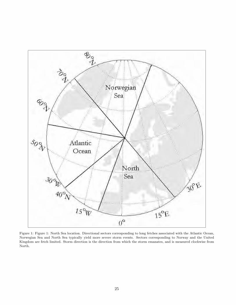
Figure 1: Figure 1: North Sea location. Directional sectors corresponding to long fetches associated with the Atlantic Ocean,Norwegian Sea and North Sea typically yield more severe storm events. Sectors corresponding to Norway and the UnitedKingdom are fetch limited. Storm direction is the direction from which the storm emanates, and is measured clockwise fromNorth.
25
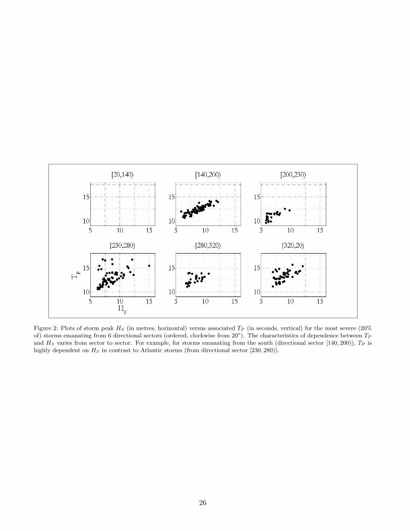
Figure 2: Plots of storm peak HS (in metres, horizontal) versus associated TP (in seconds, vertical) for the most severe (20%of) storms emanating from 6 directional sectors (ordered, clockwise from 20o). The characteristics of dependence between TP
and HS varies from sector to sector. For example, for storms emanating from the south (directional sector [140, 200)), TP ishighly dependent on HS in contrast to Atlantic storms (from directional sector [230, 280)).
26
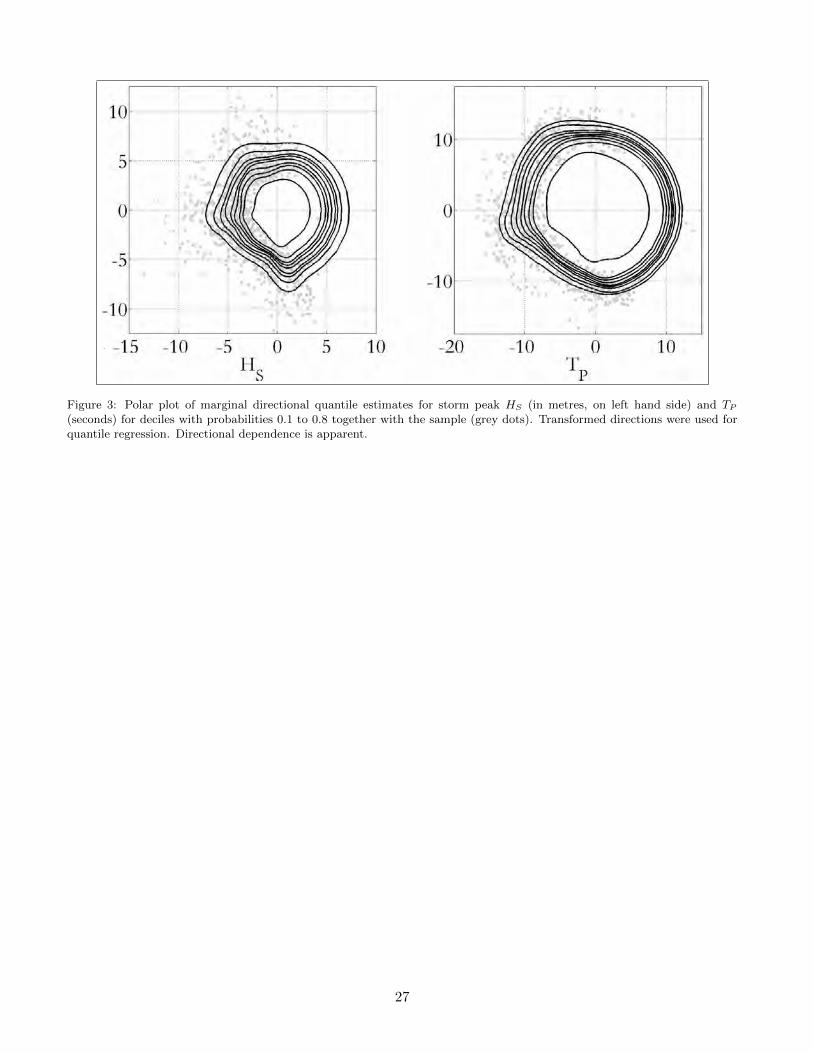
Figure 3: Polar plot of marginal directional quantile estimates for storm peak HS (in metres, on left hand side) and TP
(seconds) for deciles with probabilities 0.1 to 0.8 together with the sample (grey dots). Transformed directions were used forquantile regression. Directional dependence is apparent.
27
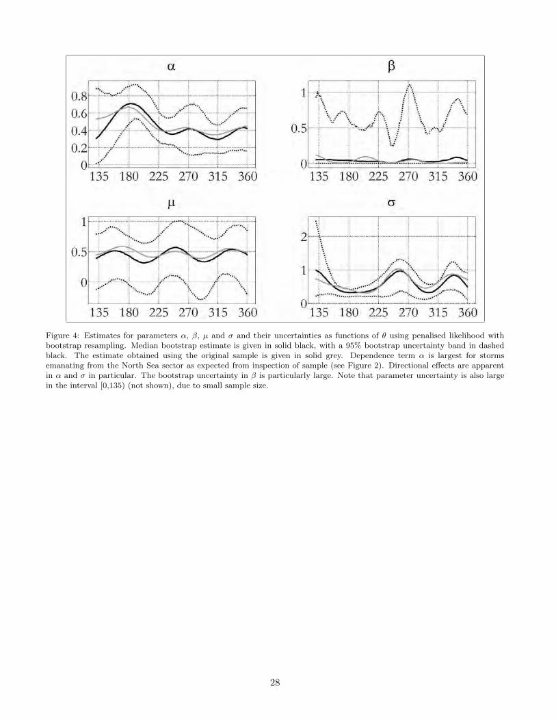
Figure 4: Estimates for parameters α, β, µ and σ and their uncertainties as functions of θ using penalised likelihood withbootstrap resampling. Median bootstrap estimate is given in solid black, with a 95% bootstrap uncertainty band in dashedblack. The estimate obtained using the original sample is given in solid grey. Dependence term α is largest for stormsemanating from the North Sea sector as expected from inspection of sample (see Figure 2). Directional effects are apparentin α and σ in particular. The bootstrap uncertainty in β is particularly large. Note that parameter uncertainty is also largein the interval [0,135) (not shown), due to small sample size.
28
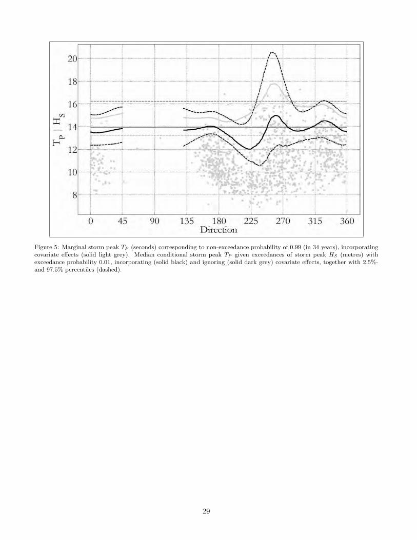
Figure 5: Marginal storm peak TP (seconds) corresponding to non-exceedance probability of 0.99 (in 34 years), incorporatingcovariate effects (solid light grey). Median conditional storm peak TP given exceedances of storm peak HS (metres) withexceedance probability 0.01, incorporating (solid black) and ignoring (solid dark grey) covariate effects, together with 2.5%-and 97.5% percentiles (dashed).
29
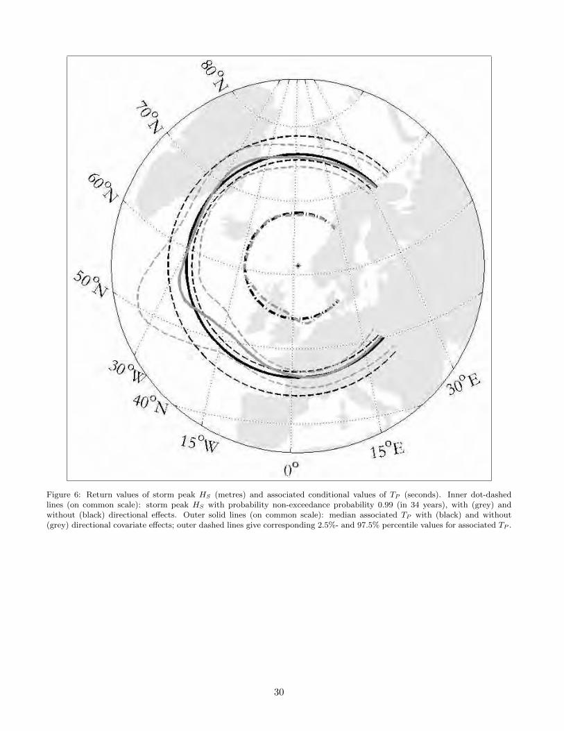
Figure 6: Return values of storm peak HS (metres) and associated conditional values of TP (seconds). Inner dot-dashedlines (on common scale): storm peak HS with probability non-exceedance probability 0.99 (in 34 years), with (grey) andwithout (black) directional effects. Outer solid lines (on common scale): median associated TP with (black) and without(grey) directional covariate effects; outer dashed lines give corresponding 2.5%- and 97.5% percentile values for associated TP .
30
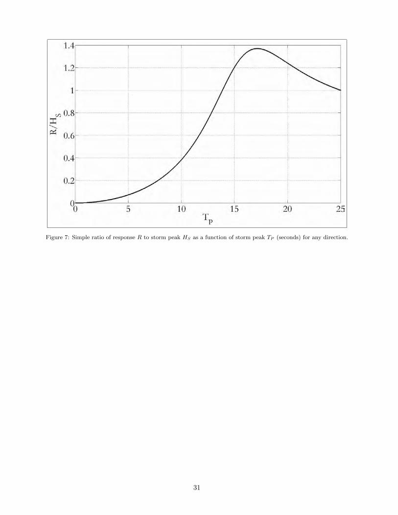
Figure 7: Simple ratio of response R to storm peak HS as a function of storm peak TP (seconds) for any direction.
31
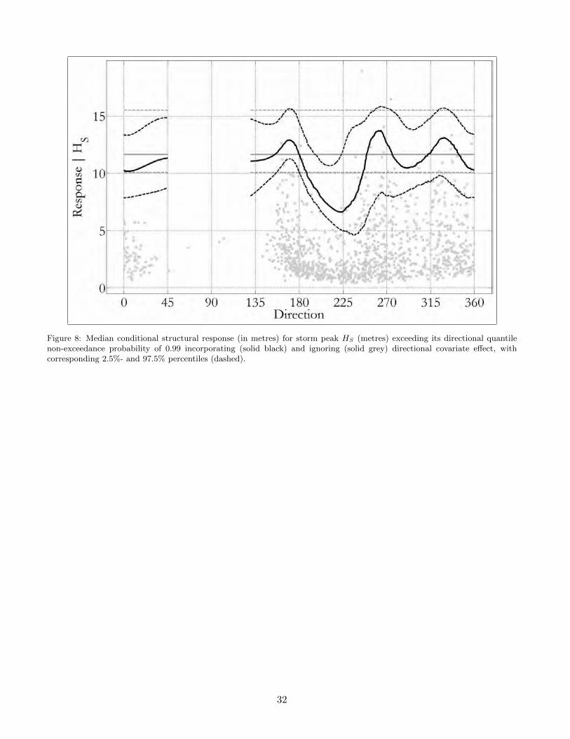
Figure 8: Median conditional structural response (in metres) for storm peak HS (metres) exceeding its directional quantilenon-exceedance probability of 0.99 incorporating (solid black) and ignoring (solid grey) directional covariate effect, withcorresponding 2.5%- and 97.5% percentiles (dashed).
32
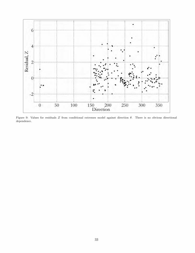
Figure 9: Values for residuals Z from conditional extremes model against direction θ. There is no obvious directionaldependence.
33
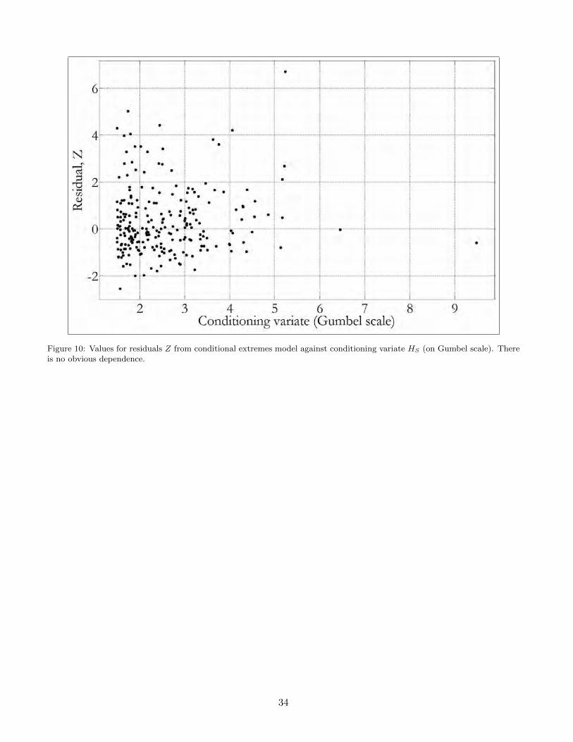
Figure 10: Values for residuals Z from conditional extremes model against conditioning variate HS (on Gumbel scale). Thereis no obvious dependence.
34
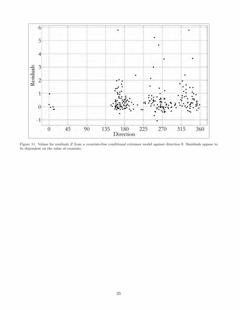
Figure 11: Values for residuals Z from a covariate-free conditional extremes model against direction θ. Residuals appear tobe dependent on the value of covariate.
35