heuristic methods to maximize network lifetime in directional sensor networks with adjustable...

Heuristic methods to maximize network lifetime in directional sensornetworks with adjustable sensing ranges

Hosein Mohamadi a, Shaharuddin Salleh a, Mohd Norsyarizad Razali bQ1

a Center of Industrial and Applied Mathematics, Universiti Teknologi Malaysia, 81310 Johor Bahru, Malaysiab Faculty of Sciences, Universiti Teknologi Malaysia, 81310 Johor Bahru, MalaysiaQ3

a r t i c l e i n f o

Article history:Received 13 January 2014Received in revised form13 June 2014Accepted 30 July 2014

Keywords:Directional sensor networksCover set formationScheduling algorithms

a b s t r a c t

During recent years, several efficient algorithms have been designed for solving the target coverageproblem in directional sensor networks (DSNs). Conventionally, it is assumed that sensors have a singlepower level. Though, it is clear that, in real applications, sensors may have multiple power levels thatdetermine different sensing ranges and power consumptions. One of the most significant challengesassociated with the DSNs is monitoring all the targets in a given area and, at the same time, maximizingthe network lifetime. In this paper, this issue is known as Maximum Network Lifetime with AdjustableRanges (MNLAR) which has not been already studied in the DSNs. In this paper, we propose twoheuristic algorithms (Algorithms 1 and 2) to solve the problem. In order to evaluate the performance ofthe proposed algorithms, extensive experiments were conducted. The obtained results were comparedto a theoretical upper bound in order to measure the quality of the solutions provided by the proposedalgorithms. The results demonstrated that Algorithm 2 was more successful than Algorithm 1 in terms ofextending the network lifetime.

& 2014 Published by Elsevier Ltd.

1. Introduction

Wireless sensor networks (WSNs) have received a great deal ofinterest in recent years due to their vast and significant applica-tions such as national security, military, and environmentalmonitoring (Cerulli et al., 2012)Q4 . A WSN is composed of a largenumber of low-cost, low-power sensor nodes that are equippedwith sensing, data processing, and communication components(Yick et al., 2008). Conventionally, in sensor networks, it is oftenassumed that sensors have a disk-like sensing range. Though, inreal world, because of equipment constraints or environmentalimpairments, sensor nodes might be limited in their sensing angleand they facilitate a sector-like sensing range (Amac Guvensan andGokhan Yavuz, 2011; Ai and Abouzeid, 2006). These types ofsensors are referred to as directional sensors (e.g., ultrasound,infrared, and video sensors). Each directional sensor can adoptseveral directions, but at a specific point of time, it can sense onlyone direction. Directional sensors are able to collect informationabout certain subregions of the whole space and they cancoordinate to perform collectively a complex sensing task (Sungand Yang, 2014).

In this study, we tackle the problem of target coverage in casesin which sensors have multiple power levels (i.e., multiple sensingranges) with the aim of extending network lifetime. The networklifetime refers to the amount of time in which the monitoring

activity can be performed. There are several challenges that arisein solving this problem in a directional sensor network (DSN).First, due to the limited sensing angle of directional sensors, theycannot sense a circular region completely; it makes the problemmore difficult compared to the WSNs (Ai and Abouzeid, 2006).Second, the energy of sensors is limited, and their batteries couldnot be easily recharged, especially in harsh environments (Ai andAbouzeid, 2006; Cai et al., 2009). Therefore, power saving mechan-isms that optimize sensor energy utilization have a great impacton extending the network lifetime. Generally, these mechanismscan be divided into two techniques: (i) scheduling in which thesensor nodes are switched between active and sleep modes, and(ii) adjusting the sensing range of the sensor nodes (Cardei et al.,2006). In recent years, several efficient scheduling algorithms havebeen proposed to solve the problem in cases where sensors have asingle power level (i.e., sensing ranges are not adjustable);whereas the technique of adjusting the sensing range of thesensor nodes (in cases where sensors have multiple power levels)has not received an adequate attention. In this study, we combineboth techniques in order to maximize the network lifetime as faras possible.

The problem of maximization of network lifetime in DSNs,which we denote as MNLAR (Maximum Network Lifetime withAdjustable Ranges), can be formally described as follows. Supposem targets with known locations and n directional sensors with

123456789

101112131415161718192021222324252627282930313233343536373839404142434445464748495051525354555657585960616263646566

67686970717273747576777879808182838485868788899091929394959697

Contents lists available at ScienceDirect

journal homepage: www.elsevier.com/locate/jnca

Journal of Network and Computer Applications

http://dx.doi.org/10.1016/j.jnca.2014.07.0381084-8045/& 2014 Published by Elsevier Ltd.

Please cite this article as: Mohamadi H, et al. Heuristic methods to maximize network lifetime in directional sensor networks withadjustable sensing ranges. Journal of Network and Computer Applications (2014), http://dx.doi.org/10.1016/j.jnca.2014.07.038i

Journal of Network and Computer Applications ∎ (∎∎∎∎) ∎∎∎–∎∎∎

www.sciencedirect.com/science/journal/10848045

www.elsevier.com/locate/jnca

http://dx.doi.org/10.1016/j.jnca.2014.07.038







adjustable sensing ranges are deployed randomly in the vicinity ofthe targets to monitor them. Initially, sensors have a certainbattery lifetime. Each sensor can be in either active or inactivemode. Each active sensor can monitor targets located in one of itsnon-overlapping directions at any given time. When a sensor is inactive mode, its power consumption is dependent on its sensingrange. On the other hand, inactive sensors do not monitor anytarget and their power consumption is negligible. The MNLARproblem deals with scheduling sensors' activity in a way tomaximize the network lifetime concerning the restriction thatthroughout the network lifetime, each target must be monitoredby the work direction of at least one active sensor.

Despite several studies recently conducted for solving thetarget coverage problem in DSNs, the problem of MNLAS has notreceived the adequate attention. In this paper, we propose twoscheduling algorithms to solve this problem. In these algorithms,we not only select the sensor directions of each cover set but alsodetermine their sensing ranges. The goal is to use a minimumsensing range to minimize the energy consumption and, at thesame time, to meet the target coverage requirement. Extensiveexperiments were conducted to examine the performance of theproposed algorithms and explore the effect of different parameterson the network lifetime. The obtained results were compared to atheoretical upper bound.

Our contributions: In this paper, we introduce the problem ofmaximum network lifetime with adjustable ranges in a DSN. Wedesign two efficient heuristics using greedy technique to solve theproblem. We evaluate the performance of the algorithms throughseveral simulations.

The remainder of this paper is organized as follows. In Section2, both background and related studies conducted on prolongingthe network lifetime are presented. In Section 3, the problem ofMNLAS is introduced. In Section 4, two new scheduling algorithmsare proposed for solving the problem. In Section 5, upper bound isintroduced. In Section 6, the performance of the proposed algo-rithms is evaluated through the simulations. Finally, Section 7concludes the paper.

2. Related work

One of the basic problems in sensor networks is coverage thatrefers to collecting different types of data from the environment.Coverage problem can be classified into two main subcategories:area coverage and target coverage (Amac Guvensan and GokhanYavuz, 2011; Zhu et al., 2012). The aim of the area coverage is thateach point in the area of interest can be continuously monitoredby at least one active sensor node. However, in some applications,only some crucial targets in the field are required to be continu-ously monitored. This study focuses on solving the target coverageproblem using both techniques of power saving, i.e., schedulingthe sensors and adjusting sensing ranges. In this section, we firstpresent a background to convey the significance of using these twotechniques in extending the network lifetime. Second, we presentsome outstanding studies conducted to solve target coverageproblem by applying these techniques to WSNs and DSNs.

2.1. Background

One of the main uses of sensor networks is collecting data ininhospitable or remote environments such as fire monitoring inforests, battlefield surveillance, and tsunami monitoring in deepsea. Since accurate placement of sensors is ruled out by cost and/orrisks considerations, under such environments, sensors are com-monly deployed in a random way. To compensate the lack ofaccuracy in such random deployment, more sensors than actually

required are distributed in the field. This over deployment causesWSNs to be more resilient to faults because some targets areredundantly monitored by multiple sensors. Each sensor is pro-vided with a limited-lifetime battery that cannot be easilyrecharged or replaced in harsh environments. Therefore, the useof power saving mechanisms for extending the network lifetime isof a great importance in the design of WSNs. Generally, thesemechanisms can be divided into two techniques: (i) schedulingsensor nodes' activity, and (ii) adjusting the sensing range ofsensor nodes (Cardei et al., 2006).

The technique of scheduling sensor nodes' activity takes theadvantage of redundancy in sensor deployment. It organizessensors into a number of cover sets each of which can monitorall the targets. Additionally, it determines the amount of time eachcover set can be activated. Afterwards, the cover sets are activatedsuccessively for a pre-determined duration. When a cover set isactive, the sensors belonging to other cover sets are in inactivemode. This significantly increases the network lifetime due to thefollowing reasons. First, inactive sensors consume considerablyless energy than the active ones. Second, if the battery of a sensorfrequently oscillates between active and inactive modes, it lasts fora longer duration (Singh and Rossi, 2013).

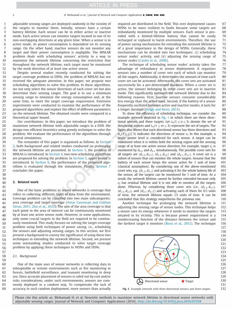
To show the efficiency of scheduling technique, we consider theexample network depicted in Fig. 1 in which there are three direc-tional sensors and three targets. Let snð1rnr3Þ denote the set ofdirectional sensors and tmð1rmr3Þ represent the set of targets. Thefigure also shows that each directional sensor has three directions anddi;jð1r jr3Þ indicates the directions of sensor si. In this example, asingle power level is considered for each sensor. A target can bemonitored when it is within both the sensing region and the sensingrange of at least one active sensor direction. For example, target t2 ismonitored by d2;2 and d3;1 simultaneously. The possible cover sets forall targets are fd1;3; d3;1g, fd1;3; d2;2g and fd2;1; d3;1g. A cover set is asubset of sensors that can monitor the whole targets. Assume that thebattery of each sensor keeps the sensor active for 1 unit of time(classical assumption). By considering one of the above-mentionedcover sets, e.g., fd1;3; d3;1g and activating it for the whole battery life ofthe sensor, all the targets can be monitored for 1 unit of time. As aresult, the network lifetime cannot be further extended because onlys2 has residual lifetime and it is not able to monitor all the targetsalone. Whereas, by considering three cover sets (i.e., fd1;3; d3;1g,fd1;3; d2;2g, and fd2;1; d3;1g) and activating each of them for 0.5 unitsof time, the network lifetime equals 1.5 units of time. It can beconcluded that this strategy outperforms the previous one.

Another technique for prolonging the network lifetime isadjusting the sensing range of sensor nodes. This technique helpsa sensor save its energy whenever it needs to monitor the targetssituated in its vicinity. This is because power requirement is anondecreasing function of the distance between the sensor andthe farthest target it monitors (Rossi et al., 2012). The technique

123456789

101112131415161718192021222324252627282930313233343536373839404142434445464748495051525354555657585960616263646566

676869707172737475767778798081828384858687888990919293949596979899

100101102103104105106107108109110111112113114115116117118119120121122123124125126127128129130131132

d1,1

d3,1

d1,2

d2,3

s2d2,2

d2,1

t1t2

t3d1,3

s3

d3,3

d3,2

Directional sensor Target

Fig. 1. Example network with three directional sensors and three targets.

H. Mohamadi et al. / Journal of Network and Computer Applications ∎ (∎∎∎∎) ∎∎∎–∎∎∎2





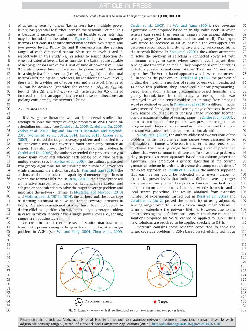
of adjusting sensing ranges (i.e., sensors have multiple powerlevels) has potential to further increase the network lifetime. Thisis because it increases the number of feasible cover sets thatmay be included in the solution. Figure 2 depicts an examplenetwork that consists of three directional sensors, two targets, andtwo power levels. Figure 2A and B demonstrates the sensingranges of each directional sensor when set at levels 1 and 2,respectively. In this study, ðdi;j; aÞ refers to sensor direction di;jwhen activated at level a. Let us consider the batteries are capableof keeping sensors active for 1 unit of time at power level 1 and0.5 units at power level 2. If we consider power level 1, there willbe a single feasible cover set (i.e., ðd1;3;1Þ; ðd3;1;1Þ) and the totalnetwork lifetime equals 1. Whereas, by considering power level 2,there will be a wider set of cover sets and a network lifetime of1.5 can be achieved (consider, for example, fðd1;3;2Þ; ðd2;2;2Þg,fðd3;1;2Þ; ðd2;1;2Þg, and fðd1;3;2Þ; ðd3;1;2Þg activated for 0.5 units oftime each). In fact, an appropriate use of the sensor directions canprolong considerably the network lifetime.

2.2. Related studies

Reviewing the literature, we can find several studies thatattempt to solve the target coverage problem in WSNs based onscheduling technique (see Cardei et al., 2005; Cardei and Du, 2005;Zorbas et al., 2010; Ting and Liao, 2010; Mostafaei and Meybodi,2013; Mohamadi et al., 2013a, 2014; Jarray, 2013). Cardei et al.(2005) introduced the target coverage problem and modeled it asdisjoint cover sets. Each cover set could completely monitor alltargets. They also proved the NP-completeness of this problem. InCardei and Du (2005), the authors extended the previous study tonon-disjoint cover sets wherein each sensor could take part inmultiple cover sets. In Zorbas et al. (2010), the authors presentedtwo greedy algorithms for maximizing the number of cover setswhile managing the critical targets. In Ting and Liao (2010), theauthors used the optimization capability of memetic algorithms toextend the network lifetime. In Jarray (2013), the author proposedan iterative approximation based on Lagrangian relaxation andsubgradient optimization to solve the target coverage problem andmaximize the network lifetime. In Mostafaei and Meybodi (2013)and Mohamadi et al. (2013a, 2014), the authors took the advantageof learning automata to solve the target coverage problem inWSNs. All above-mentioned studies have been conducted todesign efficient algorithms for solving the target coverage problemin cases in which sensors have a single power level (i.e., sensingranges are not adjustable).

On the other hand, there are several studies that have com-bined both power saving techniques for solving target coverageproblem in WSNs (see Wu and Yang, 2004; Zhou et al., 2009;

Cardei et al., 2005). In Wu and Yang (2004), two coveragealgorithms were proposed based on an adjustable model in whichsensors can select their sensing ranges from among differentsensing ranges (i.e., maximum, medium, and small). That paperwas aimed to decrease as far as possible the overlapped areabetween sensor nodes in order to save energy, hence maximizingthe network lifetime. In Zhou et al. (2009), the authors attemptedto solve the problem of selecting a connected cover set withminimum energy in cases where sensors could adjust theirsensing and transmission radius. They proposed several heuristics,including greedy formulations, Steiner Tree, and Vornoi-basedapproaches. The Vornoi-based approach was shown more success-ful in solving the problem. In Cardei et al. (2005), the problem offinding the maximum number of sensor covers was investigated.To solve this problem, they introduced a linear programming-based formulation, a linear programming-based heuristic, andgreedy formulations. In their study, a sensing model wasemployed in which a sensor could select its range from among aset of predefined values. In Dhawan et al. (2010), a different modelwas presented for adjusting the sensing range of sensors, in whicheach sensor could adjust its sensing range smoothly between0 and a maximum value of sensing range. In Cardei et al. (2006), amathematical model of the problem was presented using a linearprogram with the exponential number of variables and the linearprogram was solved using an approximation algorithm.

In Rossi et al. (2012), the authors addressed two versions of theproblem. In the first one, sensing ranges were assumed to beadjustable continuously. Whereas, in the second one, sensors hadto choose their sensing range from among a set of predefinedvalues that were common to all sensors. To solve these problems,they proposed an exact approach based on a column generationalgorithm. They employed a genetic algorithm in the columngeneration scheme in order to decrease the computation time ofthe exact approach. In Cerulli et al. (2012), the authors supposedthat each sensor could be activated in a given number ofalternative power levels that indicated different sensing rangesand power consumptions. They proposed an exact method basedon the column generation technique, a greedy heuristic, and alocal search procedure. The results obtained from extensivenumber of experiments carried out in Rossi et al. (2012) andCerulli et al. (2012) proved the superiority of using adjustablesensing ranges over the use of classical single range scheme interms of extending the network lifetime. However, due to thelimited sensing angle of directional sensors, the above-mentionedsolutions proposed for WSNs cannot be applied to DSNs. Thus,new solutions are required to be applied specially to DSNs.

Literature contains some research conducted to solve thetarget coverage problem in DSNs based on scheduling technique

123456789

101112131415161718192021222324252627282930313233343536373839404142434445464748495051525354555657585960616263646566

676869707172737475767778798081828384858687888990919293949596979899

100101102103104105106107108109110111112113114115116117118119120121122123124125126127128129130131132

d1,1

s1d3,1

d1,2

d2,3

s2

d2,2

d2,1

t1t2

d1,3

s3

d3,3

d3,2

d1,1s1

d1,2

d2,1s2

d2,2d3,1

s3

d3,2

d2,3

d3,3 d1,3

t2t1


A B

Fig. 2. Example network with three directional sensors, two targets and two power levels.

H. Mohamadi et al. / Journal of Network and Computer Applications ∎ (∎∎∎∎) ∎∎∎–∎∎∎ 3





(see Ai and Abouzeid, 2006; Cai et al., 2009; Mohamadi et al.,2013b, 2013c). Ma and Liu (2005) conducted the first study in thearea of DSNs in which they addressed sensor deploymentstrategies adopted to satisfy area coverage requirements. As thereare many studies conducted on different aspects of DSNs, wereview only those studies that have used scheduling techniquefor solving the target coverage problem with the aim of max-imizing the network lifetime (for a detailed literature review,refer to Amac Guvensan and Gokhan Yavuz, 2011). Ai andAbouzeid (2006) conducted the first study on the target coverageproblem in DSNs. They modeled the problem of maximumcoverage with the minimum sensors to maximize the numberof covered targets with a minimum number of active sensors.They proposed an integer linear programming formulation, acentralized greedy algorithm, and a distributed greedy algorithmas solutions to this problem.

In Cai et al. (2009), the authors defined the multiple directionalcover set problem and proved its NP-completeness. They proposedseveral heuristic algorithms to find non-disjoint cover sets each ofwhich covers all targets. Due to using the linear programming,their algorithms suffered from high complexity and long runningtime. In addition, they encountered too many conflicts amongdirections. In Gil and Han (2011), the authors proposed twoalgorithms for solving target coverage problem. First, a greedy-based algorithm was proposed as a baseline that could find asolution faster than other heuristic algorithms. Second, a geneticalgorithm was proposed to find the optimal cover sets. Thegreedy-based algorithm can find a solution faster compared toother heuristic algorithms; however, it may fail to find an optimalsolution due to its local search. The genetic-based algorithmrequires an upper bound on the number of covers, which cannotbe easily obtained (Mohamadi et al., 2014).

In Mohamadi et al. (2013b, 2013c), the authors proposedseveral learning automata-based scheduling algorithms for solvingthe problem. Their algorithms were composed of two phases:working direction adjustment and cover set formation. In theformer, an algorithm was proposed to choose the best workingdirection for each sensor. In the latter, several algorithms weredesigned to construct cover sets with a minimum number of activesensor directions. In the above-mentioned studies conducted onDSNs, all targets were assumed to have the same coveragerequirements. That is, the distance between the targets andsensors does not affect the coverage quality. However, in Wanget al. (2009) and Huiqiang et al. (2010), the authors assumed adifferent coverage quality for each target and employed thescheduling technique for solving the problem.

All above-mentioned studies have been conducted to designefficient algorithms for solving the target coverage problem incases where each sensor has a single power level, withoutconcerning the adjustability of the sensors' sensing range thatcan save energy in situations where a sensor should monitor onlythe targets in its vicinity. Therefore, to solve the target coverageproblem, it is necessary to design an algorithm that can use theadvantages of both techniques of power saving in such a way toextend the network lifetime as far as possible.

3. The problem of maximum network lifetime withadjustable ranges

The notations used in this study are presented in Table 1.In this paper, the following scenario is considered. A number of

targets with known locations are considered. A number of direc-tional sensors with adjustable sensing ranges are also deployed inclose proximity to the set of targets in order to monitor themcontinuously. In other words, directional sensors have multiple

distinct pre-defined sensing ranges, thus the whole targets situatedwithin these ranges are monitored with a pre-defined power level.Each directional sensor has several directions, but only one direc-tion (known as working direction) operates at each unit of time.Each directional sensor observes simultaneously all the targetslocated within both its operational range and working direction.Sensors are limited in their power and they can be activated at afinite number of alternative power levels (sensing ranges). Based onthe size, each sensing range is associated with a measure of batteryconsumption (Cerulli et al., 2012). The deployed sensors are homo-geneous in both initial battery power and the energy consumptionfor each level. The assumption is that the sensors are non-rechargeable. Since the power levels gradually extend the sensingranges of the devices, for each sensor direction di;j and each levela41, we have T ðdi;j ;bÞ DT ðdi;j ;aÞ 8b Af1;…; a�1g. Moreover, wedefine the adjusted sensor direction ðdi;j; aÞ minimal for target tj if tjAT ðdi;j ;aÞ and either a¼1 or tj =2T ðdi;j ;bÞ 8bAf1;…; a�1g.

It is noticeable that a trivial amount of energy is required forswitching a sensor from one direction to another; however, in linewith the majority of studies conducted in this field (Ai andAbouzeid, 2006; Cai et al., 2009; Gil and Han, 2011), this paperignores this small quantity of energy. In this study, a positiveparameter Δa is used for each power level a for modeling differentbattery consumptions (Cerulli et al., 2012). This parameter, Δa,signifies the ratio between battery consumption at level a andlevel 1 (which is the least powerful level and therefore the leastexpensive one). For example, Δa¼2 means that level a consumesenergy two times more than level 1. It is obvious that Δ1¼1. Wealso normalize the total battery power on the energy consumptionof level 1; that is, the battery of a sensor allows to keep it activatedfor 1 time unit if it is always set at level 1.

Problem: How to organize sensor directions into several coversets in such a way that each cover set could monitor all the targetsand, at the same time, the network lifetime could be maximized.In this paper, organizing the sensor directions refers to specifyingthe mode of each sensor direction as either active or passive andfinding the most appropriate sensing range of the active sensordirections.

Definition 1. The covering power is the ratio of the total numberof targets newly monitored by the adjusted sensor directionððdi;j; aÞÞ to the consumption ratio (Δa).

Definition 2. The covering waste is the ratio between the numberof targets already monitored in Ccur and the total number ofcovered targets.

123456789

101112131415161718192021222324252627282930313233343536373839404142434445464748495051525354555657585960616263646566

676869707172737475767778798081828384858687888990919293949596979899

100101102103104105106107108109110111112113114115116117118119120121122123124125126127128129130131132

Table 1Notations.

Notation Meaning

n Number of sensorsm Number of targetsw Number of directions per sensor, wZ1a Number of alternative power levels, aZ1si A sensor, for all iAf1;…;ngtk A target, for all kAf1;…;mgli Lifetime of sensor sidi;j jth direction of the ith sensorD Set of the directions of all the sensorsS Set of sensors, fs1;…; sngT Set of targets, ft1;…; tmgðdi;j ; aÞ Refers to sensor direction di;j activated at level a. This pair also is

defined as adjusted sensor directionTðdi;j; aÞ Refers to all the targets covered by sensor direction di;j when it is set

at level a.






Definition 3. The residual lifetime is the amount of energy eachsensor has at any given time.

4. Proposed algorithms

In this section, we developed two greedy-based algorithmsbased on an algorithm proposed in Cerulli et al. (2012) for solvingtarget coverage problem in WSNs with adjustable sensing ranges.As mentioned earlier, due to limitation in sensing angle ofdirectional sensors, the algorithms proposed for WSNs cannot beapplied to DSNs. The following modifications are performed on thealgorithms. First, the cost function was modified to be capable ofevaluating the contribution of a sensor direction instead ofevaluating that of a sensor. This was because each directionalsensor could monitor only a sector of a disk at one unit of time.Second, the algorithms were changed in such a way to avoid theselection of more than one direction and one sensing range of eachsensor for constructing a cover set. Third, a function was added tothe algorithms to improve their performance through eliminatingredundant sensor directions (if any).

In these algorithms, the network operation falls into severalrounds (the number of rounds depends on the sensor selectionstrategy) and the output of each round is a cover set that is able tomonitor all the targets. Once a cover set is constructed, anappropriate activation time within a given upper bound isassigned to the cover set to keep the feasibility of the solution.Afterwards, the energy of sensors that have a direction in the coverset is updated. The process of generating cover sets continues untilall the targets are under the full coverage of the sensor directions.The following subsections explain the algorithms in detail.

4.1. Greedy-based algorithm 1

In this section, we present the first greedy-based schedulingalgorithm (Algorithm 1) to solve the problem of MNLAR. Thealgorithm constructs at most one cover set at a time. Each coverset is constructed as follows. Initially, the algorithm starts with anempty cover set and considers all the targets as uncovered ones.Then, among all candidate sensor directions, it selects an adjustedsensor direction with the greatest contribution to cover setformation process. The selected sensor direction is added to thecover set; accordingly, the list of uncovered targets is updatedthrough the elimination of the targets monitored by the selectedsensor direction. This process continues until all the targets aremonitored. Once a cover set is constructed, the redundant sensordirections (if any) are eliminated from the cover set. Then,maximum feasible activation time of the cover set is computedbased on which the residual lifetime of sensors that exist in thecover set is updated. Next, the exhausted sensors are removedfrom the list of available sensors. The process of generating a newcover set continues until all the targets are under the full coverageof the sensor directions.

The pseudo code of the algorithm is shown in Algorithm 1. Inthe following, we explain this pseudo code in detail and introducesome notations used in this paper. Line 1 includes the inputparameters. Granularity factor gf Að0;1� signifies a maximum valueof working time (activation time) that will be assigned to eachconstructed cover set. In order to weight the different sensordirection contribution criteria, the γ vector is used. Parameter Liinitialized in lines 2–4 represents the amount of residual lifetime foreach sensor si. The set SOL and the value LF initialized in lines 5 and6 contain the cover sets with their related working times. The setSOL and the value LF are returned as solution and the maximumnetwork lifetime, respectively. The Dcur set initialized in line7 contains the set of directions of available sensors. Line 8 checks

whether the available sensor directions can still monitor all thetargets and construct a new cover set Ccur. The Tcur and Ccur setsinitialized in lines 9 and 10 keep the list of uncovered targets andthat of the sensor directions that have already been included in Ccur,respectively. Parameter Selected initialized in line 12 signifies theadjusted sensor direction with the greatest contribution. ParameterMax_CF initialized in line 13 represents the amount of contributionof the selected sensor direction. Parameter Pselected used in line 22represents the set of targets covered by the adjusted sensordirection ðdi;j; aÞ.

In order to generate a cover set (lines 11–24), the adjustedsensor direction with the greatest contribution should be itera-tively selected until all the targets are monitored. For this purpose,at each iteration of the algorithm, the contribution of eachadjusted sensor direction ðdi;j; aÞ is evaluated based on a costfunction that consists of three different criteria: covering power,covering waste, and residual lifetime (see Section 4.1.1). Thesecriteria are considered in order to (i) evaluate the trade-offbetween the number of new covered targets and consumptionratio Δa; (ii) measure the percentage of sensor directions thatwould be monitored redundantly if ðdi;j; aÞ are added to the currentcover set; and (iii) compute the overall amount of its residualenergy.

After the evaluation, at first, the sensor direction with thegreatest contribution is selected and added to the cover set that isbeing formed (i.e., Ccur). Then, the targets covered by the selecteddirection are removed from the set of uncovered targets (i.e., Tcur).Finally, not only the selected direction but also the other directionsof the same sensor are removed from the set of available directionsin order to avoid both the selection of more than one direction ofeach sensor and the selection of more than one sensing range ofeach sensor simultaneously. This process continues until a coverset is formed.

After forming a cover set, the redundant sensor directions ofthe constructed cover set are eliminated (if any) in such a way thatthey could be used again to form new cover sets. The aim of thisprocess is increasing the number of cover sets and, consequently,prolonging the network lifetime. A direction of the cover set isredundant if after its removal, all the targets are still under fullcoverage. Using a simple exclusion, the redundant directions areremoved from the constructed cover sets; each direction of thecover set is checked to find whether it is redundant or not, and theredundant ones will be removed.

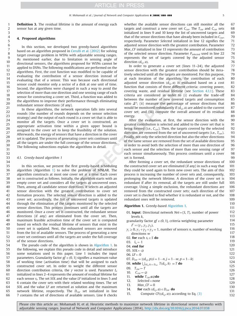
Algorithm 1. Greedy-based Algorithm 1.

01. Input: Directional network Net¼(S, T), number of powerlevels k,

granularity factor gf Að0;1�, criteria weighting parameterΓ ¼ ðγ1; γ2; γ3Þ,

γiZ0, γ1þγ2þγ3 ¼ 1, number of sensors n, number of workingdirections w

02. for each siAS do03. lsi’104. end for05. SOL’∅06. LF’007. Dcur ¼ fðdi;j; pÞji¼ 1⋯n; j¼ 1⋯w; p¼ 1⋯kg08. while ⋃ðdi;j ;kÞADcur

Tðdi;j; kÞ � T do09. Tcur’T10. Ccur’∅11. while Tcur≢∅do12. Selected¼none13. Max_CF ¼ 014. for each ðdi;j; aÞADcur do15. Compute CFððdi;j; aÞÞ according to Eq. (3)

123456789

101112131415161718192021222324252627282930313233343536373839404142434445464748495051525354555657585960616263646566

676869707172737475767778798081828384858687888990919293949596979899

100101102103104105106107108109110111112113114115116117118119120121122123124125126127128129130131132






16. if CF4Max_CF then17. Max_CF ¼ CF18. Selected¼ ðdi;j; aÞ19. end if20. end for21. Ccur ¼ Ccur [ Selected22. Tcur ¼ Tcur�PSelected

23. Dcur ¼Dcur�Selected [ the other directions and sensingranges of the same sensor

24. end while25. Remove redundant sensor directions26. WTl ¼max feasible activation time rgf for Ccur27. LF’LFþWTl

28. for each ðdi;j; aÞACcur do

29. lsi’lsi �ðΔaWTlÞ30. if lsi ¼ 0 then31. S’S�si32. end if33. end for34. Dcur ¼ fðdi;j; kÞg for the available sensors35. SOL’SOL⋃fðCcur ;WTlÞg36. end while37. return (SOL, LF)

After elimination of redundant sensors, the updated cover set isassigned with a working time. This unit of time is added to thetotal network lifetime. In line 27, the network lifetime is updated.Next, the residual energy of those sensors that have a direction inthe cover set is updated based on the maximum feasible workingtime, and the sensors without any residual energy are eliminatedfrom the set of available sensors (see lines 28–33). In more detail,Ccur will be activated for WTl ¼ gf if Li�Δagf Z0 for eachðdi;j; aÞACcur . Otherwise, consider the adjusted sensor of Ccur thatminimizes Li=Δ

a; let us call it ðsh; bÞ. We set WTl ¼ Lsh=Δb; this

ensures a feasible working time for each ðdi;j; aÞACcur . Line 34updates the list of available sensor directions in Dcur set. In line 35,the newly constructed cover set and its working time are added tothe solution. Finally, in line 37, the constructed cover sets and theiractivation times are returned as the output of the algorithm.

4.1.1. Adjusted sensor directions contributionIn order to determine the contribution of each sensor direction,

three criteria, namely Covering Power (CP), Covering Waste (CW),and Residual Lifetime (RL) (adapted from Cerulli et al., 2012) aretaken into account. In Cerulli et al. (2012), these criteria were usedto determine the contribution of a sensor to the process of coverset formation; whereas in our study, they are used to calculate thecontribution of one direction of a sensor. This is because (aspreviously mentioned) at any given time, only one direction of adirectional sensor can be activated. Each criterion returns a scorefor each candidate adjusted sensor direction. Then, these scoresare combined to evaluate the overall contribution of the adjustedsensor direction. In the following, we elaborate each criterion.

Covering power: While a new cover set is being formed, for eachadjusted sensor direction ðdi;j; aÞ, the CP score is defined as the ratiobetween the total number of uncovered targets monitored by theadjusted sensor direction ðdi;j; aÞ and consumption ratio Δa; that is,

CPðdi;j; aÞ ¼jT ðdi;j ;aÞ⋂Tcur j

Δa ð1Þ

Based on this criterion, the maximum CP score determines thegreatest contribution. This criterion gives a higher score to the sensorsthat have relevant covering capabilities, while it penalizes the sensordirections with high power levels that do not bring considerable

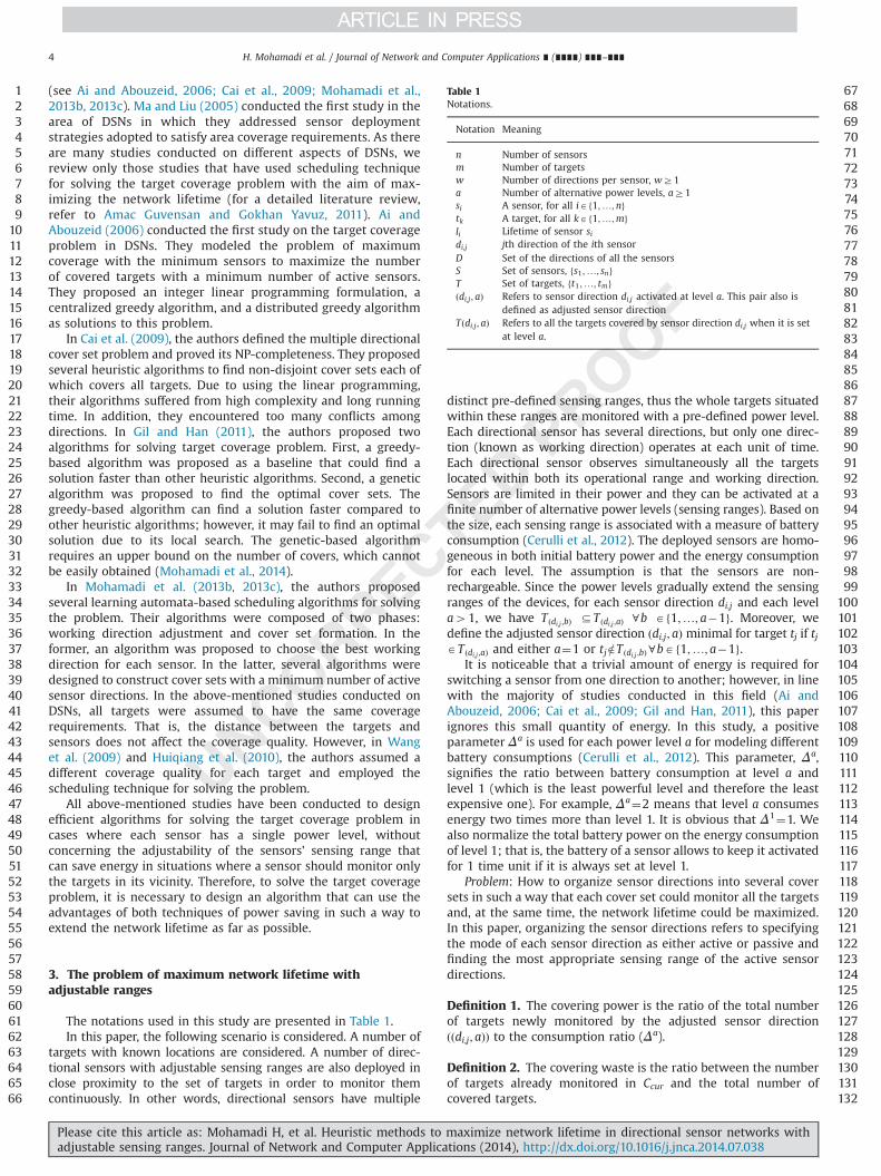
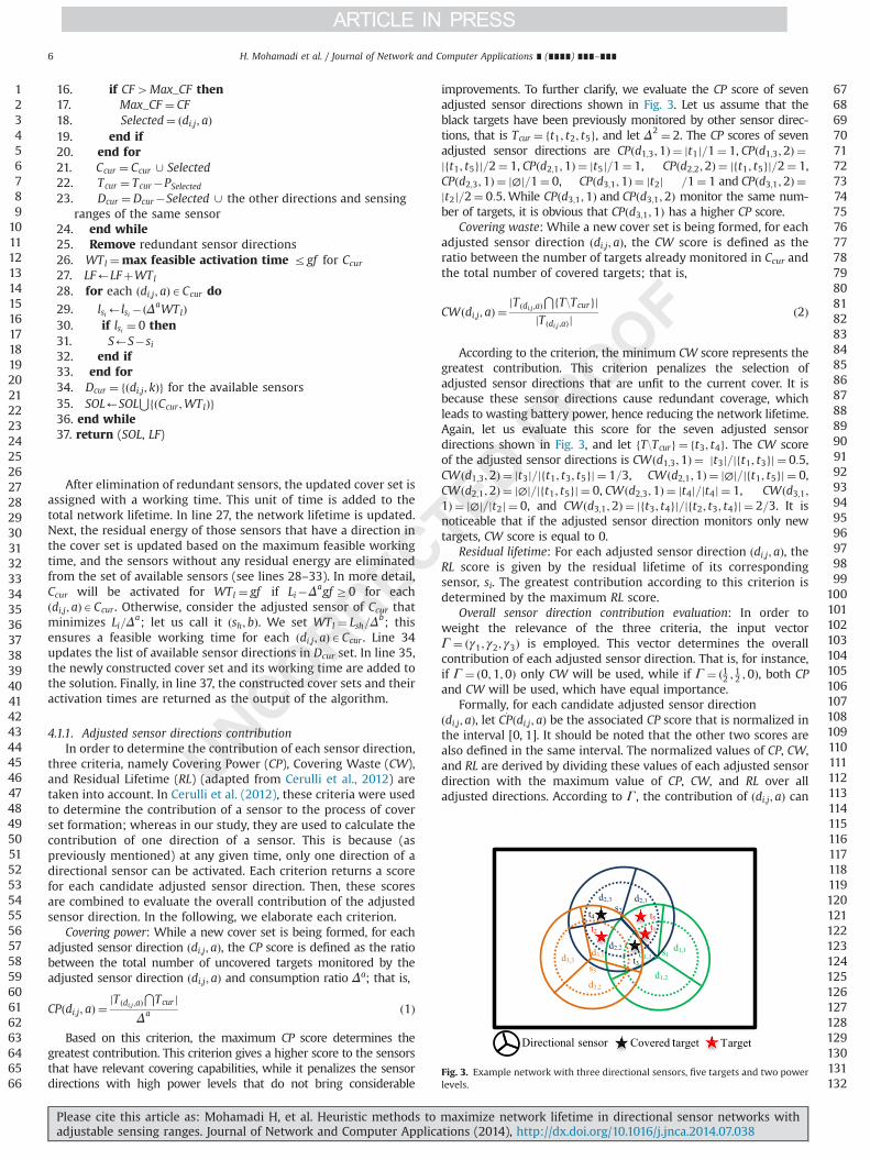
improvements. To further clarify, we evaluate the CP score of sevenadjusted sensor directions shown in Fig. 3. Let us assume that theblack targets have been previously monitored by other sensor direc-tions, that is Tcur ¼ ft1; t2; t5g, and let Δ2 ¼ 2. The CP scores of sevenadjusted sensor directions are CPðd1;3;1Þ ¼ jt1j=1¼ 1, CPðd1;3;2Þ ¼jft1; t5gj=2¼ 1, CPðd2;1;1Þ ¼ jt5j=1¼ 1, CPðd2;2;2Þ ¼ jft1; t5gj=2¼ 1,CPðd2;3;1Þ ¼ j∅j=1¼ 0, CPðd3;1;1Þ ¼ jt2j =1¼ 1 and CPðd3;1;2Þ ¼jt2j=2¼ 0:5. While CPðd3;1;1Þ and CPðd3;1;2Þ monitor the same num-ber of targets, it is obvious that CPðd3;1;1Þ has a higher CP score.

Covering waste: While a new cover set is being formed, for eachadjusted sensor direction ðdi;j; aÞ, the CW score is defined as theratio between the number of targets already monitored in Ccur andthe total number of covered targets; that is,

CWðdi;j; aÞ ¼jT ðdi;j ;aÞ⋂fT\Tcurgj

jT ðdi;j ;aÞjð2Þ

According to the criterion, the minimum CW score represents thegreatest contribution. This criterion penalizes the selection ofadjusted sensor directions that are unfit to the current cover. It isbecause these sensor directions cause redundant coverage, whichleads to wasting battery power, hence reducing the network lifetime.Again, let us evaluate this score for the seven adjusted sensordirections shown in Fig. 3, and let fT\Tcurg ¼ ft3; t4g. The CW scoreof the adjusted sensor directions is CWðd1;3;1Þ ¼ jt3j=jft1; t3gj ¼ 0:5,CWðd1;3;2Þ ¼ jt3j=jft1; t3; t5gj ¼ 1=3, CWðd2;1;1Þ ¼ j∅j=jft1; t5gj ¼ 0,CWðd2;1;2Þ ¼ j∅j=jft1; t5gj ¼ 0, CWðd2;3;1Þ ¼ jt4j=jt4j ¼ 1, CWðd3;1;1Þ ¼ j∅j=jt2j ¼ 0, and CWðd3;1;2Þ ¼ jft3; t4gj=jft2; t3; t4gj ¼ 2=3. It isnoticeable that if the adjusted sensor direction monitors only newtargets, CW score is equal to 0.

Residual lifetime: For each adjusted sensor direction ðdi;j; aÞ, theRL score is given by the residual lifetime of its correspondingsensor, si. The greatest contribution according to this criterion isdetermined by the maximum RL score.

Overall sensor direction contribution evaluation: In order toweight the relevance of the three criteria, the input vectorΓ ¼ ðγ1; γ2; γ3Þ is employed. This vector determines the overallcontribution of each adjusted sensor direction. That is, for instance,if Γ ¼ ð0;1;0Þ only CW will be used, while if Γ ¼ ð12 ; 12 ;0Þ, both CPand CW will be used, which have equal importance.

Formally, for each candidate adjusted sensor directionðdi;j; aÞ, let CP! ðdi;j; aÞ be the associated CP score that is normalized inthe interval [0, 1]. It should be noted that the other two scores arealso defined in the same interval. The normalized values of CP, CW,and RL are derived by dividing these values of each adjusted sensordirection with the maximum value of CP, CW, and RL over alladjusted directions. According to Γ, the contribution of ðdi;j; aÞ can

123456789

101112131415161718192021222324252627282930313233343536373839404142434445464748495051525354555657585960616263646566

676869707172737475767778798081828384858687888990919293949596979899

100101102103104105106107108109110111112113114115116117118119120121122123124125126127128129130131132

d1,1d3,1 d1,3

s2

t1t2

d1,2s3

d3,3

d3,2

Directional sensor Covered target

t3

t5t4

Target

Fig. 3. Example network with three directional sensors, five targets and two powerlevels.






be defined as the convex combination as follows:

CFðdi;j; aÞ ¼ γ1CP! ðdi;j; aÞþγ2ð1�CW! ðdi;j; aÞÞþγ3RL

! ðdi;j; aÞ ð3Þ

Therefore, at each iteration, algorithm chooses the adjusted sensordirection that maximizes this value, CFðdi;j; aÞ.

So far, the first greedy-based algorithm and its contribution tosolving the problem of MNLAR have been explained. The criticalsensors set an upper bound on the network lifetime and theexhaustion of their energy causes the network operation to beterminated. Therefore, they should be managed efficiently. Sincethe first greedy-based algorithm (Algorithm 1) was not able tomanage the critical sensor directions, the second greedy-basedalgorithm (Algorithm 2) was proposed to overcome this short-coming and achieve a longer network lifetime. Additionally,compared to Algorithm 1, Algorithm 2 requires less computationduring the process of cover set formation. This is because, forconstructing a cover set, at each iteration, Algorithm 1 computesthe cost function for all sensor directions and selects the sensordirection with the best contribution to the process of cover setformation. Whereas, Algorithm 2 first finds a critical target, thencomputes the cost function of only those sensor directions thatmonitor the critical target. This causes a significant reduction inthe number of computations.

4.2. Greedy-based Algorithm 2

In this section, we present the second greedy-based algorithm inorder to solve the problem of MNLAR. Similar to Algorithm 1, thenetwork operation of this algorithm falls into a number of roundsand the outcome of each round is a cover set. In this algorithm, theprocess of generating a cover set can be explained as follows. Thealgorithm starts initially with an empty cover set and considers all thetargets as uncovered ones. The algorithm chooses a critical target (i.e.,a target covered by sensor directions that have the least amount ofresidual energy) and finds an adjusted sensor direction that has thegreatest contribution to monitoring the critical target. Then, the sensordirection is added to the cover set; accordingly, the list of uncoveredtargets is updated through removing the critical target and the othertargets monitored by the selected sensor direction. The process ofselecting a critical target and finding a sensor direction to monitor thiscritical target is repeated until all the targets are monitored. Then, theprocesses of removing the redundant sensor directions and computingthe maximum activation time of the generated cover set are per-formed similar to Algorithm 1. The algorithm continues until theavailable sensor directions are capable of constructing a new cover set.

The pseudo code of the algorithm is shown in Algorithm 2. Inthe following, the steps of constructing a cover set in Algorithm 2is explained. First, a critical target is identified in line 2. Then,the adjusted sensor direction with the greatest contribution isselected among the sensor directions that cover the critical targetbased on Eq. (3) in line 3. Next, the selected adjusted sensordirection is added to the cover set Ccur in line 4. After that, the listof uncovered targets are updated in line 5. Finally, the list ofavailable sensor directions is updated in line 6. This processcontinues until the selected sensor directions cover all the targets.

Similar to Algorithm 1, after forming a cover set, the redundantsensor directions of the cover set are eliminated (if any). Then, aworking time is assigned to the cover set and the value of thistime is added to the total network lifetime. Next, the residualenergy of the sensors that have a direction in the cover set isupdated, and the sensors without any residual energy are removedfrom the set of available sensors. Finally, the generated cover setsand their working times are returned as an output of thealgorithm.

Algorithm 2. Cover set formation step of Algorithm 2.

01. while Tcur≢∅ do02. Find a critical target tcATcur

03. Select ðdi;j; aÞ that covers target tc and has the maximumcontribution based on Eq. (3)

04. Ccur ¼ Ccur [ ðdi;j; aÞ05. Tcur ¼ Tcur� the targets covered by the adjusted sensor

direction ðdi;j; aÞ06. Dcur ¼Dcur�ðdi;j; aÞ [ the other directions and sensing

ranges of the same sensor07. end while

The complexity of the proposed greedy algorithms isOðn2w2m2ðE=e1ÞÞ. The number of iterations of the while loop (lines8…36) is upper-bounded by nðE=e1Þ, which is corresponding tocases where all the targets are monitored by all sensor directionswith their first sensing ranges. The complexity of the inner whileloop (lines 11…24) is upper-bounded by Oðn2w2m2Þ.

4.3. Critical targets

Critical targets are bottleneck to network lifetime; they definean upper bound on the maximum operation time of the network.That is, when the energy of sensors that cover a critical target runsout, the target cannot be monitored any longer, consequently, thenetwork lifetime ends. To find critical targets, an upper bound Utjis evaluated based on the amount of time for which each target tjcan be monitored by the residual lifetime of the sensors. In moredetail, for each target tjATcur and each sensor direction di;jADcur

such that tjATðdi;j; kÞ, let aij be the power level such that ðdi;j; aijÞ isminimal for tj. On the other words, the power level with the lowestpossible consumption level is considered for each covering sensorbecause this power level can maximize the covering time. Thecritical target, tc, is defined as follows:

tc ¼ argmin; ðUtj Þ tjATcur ð4Þ

where

Utj ¼ ∑di;j ADcur jtj ATðdi;j ;kÞ

lsiΔaij

ð5Þ

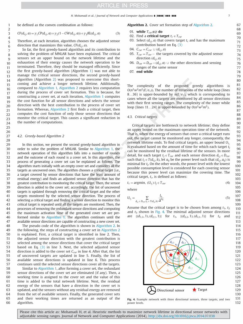
Assume that the critical target is to be chosen from among t1, t2and t3 shown in Fig. 4. The minimal adjusted sensor directionsare fðd1;3;1Þ; ðd2;1;1Þg for t1, fðd2;2;1Þ; ðd3;1;1Þg for t2 and

123456789

101112131415161718192021222324252627282930313233343536373839404142434445464748495051525354555657585960616263646566

676869707172737475767778798081828384858687888990919293949596979899

100101102103104105106107108109110111112113114115116117118119120121122123124125126127128129130131132

d1,1d3,1 d1,3

d2,3 s2

d2,2

t1t2

d1,2s3

d3,3

d3,2


t3

Fig. 4. Example network with three directional sensors, three targets, and twopower levels.






fðd1;3;2Þ; ðd2;2;1Þg, ðd3;1;2Þg for t3. Let us assume that Δ2 ¼ 2 (recallthat by definition Δ1 ¼ 1, and ls1 ¼ 1, ls2 ¼ 0:5 and ls3 ¼ 0:25. Then,we have Ut1 ¼ ðls1 þ ls2 Þ=Δ1 ¼ 1:5, Ut2 ¼ ðls2 þ ls3 Þ=Δ1 ¼ 0:75 andUt3 ¼ ððls1 þ ls3=Δ

2ÞÞþ ls2=Δ1 ¼ 1:125. Therefore, t2 is the critical

target.

5. Upper bound computation

To evaluate the quality of the solutions provided by theproposed algorithms, a theoretical upper bound U is calculated.This upper bound is the same as the one explained for the criticaltarget selection. This calculation is performed when lsi ¼ 1 for eachsensor direction di;j in D. Let us consider a target tj and a sensordirection di;j such that tjATðdi;j; kÞ, let aij be the power level suchthat ðdi;j; aijÞ is minimal for tj. Then, we have

U ¼minðUtj Þ; tjAT ð6Þ

where

Utj ¼ ∑di;j ADjtj ATðdi;j ;kÞ

1Δaij

ð7Þ

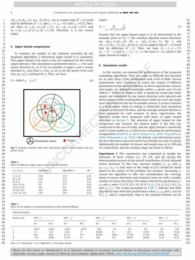
Assume that the upper bound target is to be determined in theexample given in Fig. 5. The minimal adjusted sensor directionsare fðd2;3;1Þ; ðd3;1;2Þg for t1, fðd2;2;1Þ; ðd3;1;1Þg for t2 andfðd1;3;2Þ; ðd2;2;1Þg, ðd3;1;2Þg for t3. Let us suppose that Δ2 ¼ 2 (recallthat by definition Δ1 ¼ 1). Then, we have Ut1 ¼ 1

1 þ12 ¼ 1:5,

Ut2 ¼ 1þ11 ¼ 2 and Ut3 ¼ 1þ1

2 þ11 ¼ 2. We have U¼1.5, which is the

upper bound of target t1.

6. Simulation results

In this section, we evaluate the performance of the proposedscheduling algorithms. They are coded in MATLAB and executedon an Intel Xeon 2 GHz workstation with 4 GB of RAM. Severalexperiments were conducted to assess the impact of differentparameters on the network lifetime. In these experiments, sensorsand targets are disposed randomly within a square area of size1000 m n 1000 m to model a DSN. It should be noted that thosetargets not monitored by any sensor direction were ignored andthose sensors whose working directions could not cover any targetwere removed from the list of available sensors. A sensor is knownas a dead sensor when its energy is exhausted. Each simulationscenario is executed 50 times, and the average network lifetime isthen computed for each scenario. In these experiments, theobtained results were compared with those of upper bounddescribed in Section 5. The selection of upper bound for thiscomparison was because the present paper is the first oneconducted in this area of study, and the upper bound is commonlyused in many studies as a criterion for evaluating the performanceof algorithms (Cerulli et al., 2012; Zorbas et al., 2010; Ting and Liao,2010; Mohamadi et al., 2013c). By default, each directional sensorhas four directions and each sensor has initially one unit of energy.Additionally, the number of sensors and targets was set to 100 and10, respectively, and the sensing range was fixed to 200 m.

Experiment 1. This experiment was conducted to weight therelevance of three criteria (i.e., CP, CW, and RL) during thedetermination process of the overall contribution of each adjustedsensor direction. To this end, constant weights γ1, γ2, and γ3ðγ1þγ2þγ3 ¼ 1Þ that were in the range of (0,1) should be tunedbased on the nature of the problem. For instance, increasing γ1caused the algorithm to take into consideration the coveragestatus of sensor directions and construct cover set with a smallernumber of sensor directions. The values selected for parameters γ1,γ2, and γ3 were (1, 0, 0), (0, 1, 0), (0, 0, 1), ð12 ; 12 ;0Þ, ð12 ;0; 12 Þ, ð0; 12 ; 12 Þ,and ð13 ; 13 ; 13 Þ. The results presented in Table 2 indicate that bothalgorithms have their best performance when γ1, γ2, and γ3 are setto 1

2 ,12 , and 0, respectively. That is, the network lifetime can be

123456789

101112131415161718192021222324252627282930313233343536373839404142434445464748495051525354555657585960616263646566

676869707172737475767778798081828384858687888990919293949596979899

100101102103104105106107108109110111112113114115116117118119120121122123124125126127128129130131132

Table 2Effect of different weight values on the network lifetime.

ðγ1; γ2; γ3Þ Algorithm 1 Algorithm 2 UB

(1, 0, 0) 3.58 3.73 4.25(0, 1, 0) 3.45 3.71 4.25(0, 0, 1) 3.21 3.52 4.25(1/2, 1/2, 0) 3.6 3.77 4.25(1/2, 0, 1/2) 3.27 3.4 4.25(0, 1/2, 1/2) 3.43 3.64 4.25(1/3, 1/3, 1/3) 3.26 3.41 4.25

d1,1d3,1 d1,3

d2,3 s2

d2,2

t1

t2

d1,2s3

d3,3

d3,2


t3

Fig. 5. Example network with three directional sensors, three targets and twopower levels.

Table 3Effect of the number of working directions on the network lifetime.

Network lifetime

Power level WD ¼1 WD ¼ 2 WD ¼ 3 WD ¼ 4 WD ¼ 5

Al 1 Al 2 Al 1 Al 2 Al 1 Al 2 Al 1 Al 2 Al 1 Al 2

1 4.675 4.675 4.125 4.075 3.85 3.9 3.8 3.9 3.6 3.672 7.3 7.25 9.25 9 10.925 11 13.6 13.575 15.4 15.223 8.15 8.65 11.175 11.7 14.325 14.05 17.675 17.275 19.92 20.174 7.95 8.925 11.575 12 14.8 15.1 18.675 19.025 21.47 21.97

Note: Al 1, Algorithm 1; Al 2, Algorithm 2; UB, Upper bound.






maximally extended when the algorithms simultaneously considerboth covering power and covering waste of directional sensors.Therefore, values ð12 ; 12 ;0Þ are applied to the following experiments.

Experiment 2. This experiment was designed to examine theimpact of the number of working directions on the networklifetime. For this purpose, the number of working directions wasranged between 1 and 5 with incremental step 1, and the numberof sensors was set to 300. Here, the initial energy is set to a valueequal to the number of working directions. The obtained resultsshown in Table 3 indicates that there is a direct relationshipbetween the number of working directions and network lifetime.That is, more number of working directions leads to moreprolonged the network lifetime.

Experiment 3. This experiment was carried out to examine theeffects of the number of sensors on the network lifetime. Thenumber of sensors was ranged from 100 to 300 with incrementalstep 50. The number of power levels was ranged between 1 and4 with incremental step 1. It should be noted that when powerlevel is equal to 1, all sensors have a fixed sensing range. Theobtained results presented in Fig. 6 shows that with an increase inthe number of sensors, the network lifetime increases. This isbecause with deploying more sensors, each target is covered bymore sensors, hence forming more cover sets. The results alsoshows that multiple power levels had a considerable impact on thenetwork lifetime, especially when increasing power level from 1 to2, 3 or 4. Once the power levels increases from 3 sensing ranges to4 power levels, the network lifetime increases at a lower rate. Thesimulation results justify the contribution of this paper, showingthat multiple power levels can greatly extend the network life-time. The obtained results presented in Table 4 show thatAlgorithm 1 was able to generate a cover set in a less amount oftime compared to Algorithm 1. The reason is that generating acover set in Algorithm 2 depends on the evaluation of only critical

sensor directions, while in Algorithm 1, all sensor directionsshould be evaluated at each stage. In this experiment, Algorithm2 was found more efficient in terms of extending the networklifetime. It was due to managing the critical sensor directions.

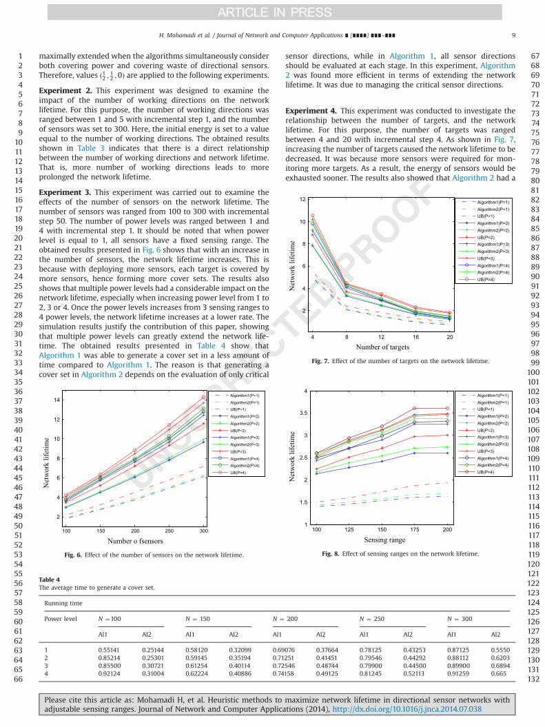
Experiment 4. This experiment was conducted to investigate therelationship between the number of targets, and the networklifetime. For this purpose, the number of targets was rangedbetween 4 and 20 with incremental step 4. As shown in Fig. 7,increasing the number of targets caused the network lifetime to bedecreased. It was because more sensors were required for mon-itoring more targets. As a result, the energy of sensors would beexhausted sooner. The results also showed that Algorithm 2 had a

123456789

101112131415161718192021222324252627282930313233343536373839404142434445464748495051525354555657585960616263646566

676869707172737475767778798081828384858687888990919293949596979899

100101102103104105106107108109110111112113114115116117118119120121122123124125126127128129130131132

Table 4The average time to generate a cover set.

Running time

Power level N ¼100 N ¼ 150 N ¼ 200 N ¼ 250 N ¼ 300

Al1 Al2 Al1 Al2 Al1 Al2 Al1 Al2 Al1 Al2

1 0.55141 0.25144 0.58120 0.32099 0.69076 0.37664 0.78125 0.43253 0.87125 0.55502 0.85214 0.25301 0.59145 0.35194 0.71251 0.41451 0.79546 0.44292 0.88112 0.62033 0.85500 0.30721 0.61254 0.40114 0.72546 0.48744 0.79900 0.44500 0.89900 0.68944 0.92124 0.31004 0.62224 0.40886 0.74158 0.49125 0.81245 0.52113 0.91259 0.665

100 150 200 250 300

2

4

6

8

10

12

14Algorithm1(P=1)

Algorithm2(P=1)

UB(P=1)

Algorithm1(P=2)

Algorithm2(P=2)

UB(P=2)

Algorithm1(P=3)

Algorithm2(P=3)

UB(P=3)

Algorithm1(P=4)

Algorithm2(P=4)

UB(P=4)

Number o fsensors

Net

wor

k lif

etim

e

Fig. 6. Effect of the number of sensors on the network lifetime.

100 125 150 175 2001

1.5

2

2.5

3

3.5

4Algorithm1(P=1)Algorithm2(P=1)UB(P=1)Algorithm1(P=2)Algorithm2(P=2)UB(P=2)Algorithm1(P=3)Algorithm2(P=3)UB(P=3)Algorithm1(P=4)Algorithm2(P=4)UB(P=4)

Sensing range

Net

wor

klif

etim

e

Fig. 8. Effect of sensing ranges on the network lifetime.

4 8 12 16 20

2

4

6

8

10

12 Algorithm1(P=1)Algorithm2(P=1)UB(P=1)Algorithm1(P=2)Algorithm2(P=2)UB(P=2)Algorithm1(P=3)Algorithm2(P=3)UB(P=3)Algorithm1(P=4)Algorithm2(P=4)UB(P=4)

Number of targets

Net

wor

k lif

etim

e

Fig. 7. Effect of the number of targets on the network lifetime.






better performance than Algorithm 1 in terms of extending net-work lifetime.

Experiment 5. This experiment examined the impact of thesensing range on the network lifetime. The sensing range wasvaried between 100(m) and 200(m) with incremental step 25 (m).The results presented in Fig. 8 indicate that increasing the sensingrange causes the network lifetime to be enhanced. This is becauseonce the sensing range enlarges, sensor nodes are capable ofmonitoring more targets, and as a result, fewer sensors arerequired to cover the whole targets. The obtained results alsoshowed that by increasing the sensing range, Algorithm 2 couldachieve a longer network lifetime than Algorithm 1.

7. Conclusion

This paper investigated the problem of target coverage in casesin which the sensors have multiple directions and multiplesensing ranges. To solve this problem, we proposed two greedy-based scheduling algorithms (Algorithms 1 and 2) that were aimedto select the appropriate sensor directions and sensing ranges in away to meet the requirement of target coverage problem and, atthe same time, maximize the network lifetime. In order toevaluate the performance of the proposed algorithms, we carriedout several experiments. The obtained results showed thatAlgorithm 2 outperformed Algorithm 1 in terms of extending thenetwork lifetime due to appropriately managing the criticaltargets. The simulation results justified the contribution of thispaper, showing that multiple directional sensors and multiplepower levels can greatly extend the network lifetime. In futurestudies, we intend to develop appropriate metaheuristic algo-rithms for solving the problem considered in this study.

Uncited reference

Mohamadi et al. (2013d)Q2 .

Acknowledgments

The authors would like to thank Universiti Teknologi Malaysiaand the Malaysian Ministry of Education for providing funds andsupport with research Grant nos. 01G14 and 04H43 for thisresearch.

References

Ai J, Abouzeid A. Coverage by directional sensors in randomly deployed wirelesssensor networks. J Combin Optim 2006;11:21–41.

Amac Guvensan M, Gokhan Yavuz A. On coverage issues in directional sensornetworks: a survey. Ad Hoc Netw 2011;9:1238–55.

Cai Y, Lou W, Li M, Li X-Y. Energy efficient target-oriented scheduling in directionalsensor networks. IEEE Trans Comput 2009;58:1259–74.

Cardei M, Du D-Z. Improving wireless sensor network lifetime through poweraware organization. Wireless Netw 2005;11:333–40.

Cardei M, Thai MT, Yingshu L, Weili W. Energy-efficient target coverage in wirelesssensor networks. In: Proceedings of 24th annual joint conference of the IEEEcomputer and communications societies (INFOCOM); 2005. p. 1976–84.

Cardei M, Wu J, Lu M, Pervaiz MO. Maximum network lifetime in wireless sensornetworks with adjustable sensing ranges. In: Proceedings of internationalconference on wireless and mobile computing, networking and communica-tions, vol. 3; 2005. p. 438–45.

Cardei M, Wu J, Lu M. Improving network lifetime using sensors with adjustablesensing ranges. Int J Sens Netw 2006;1:41–9.

Cerulli R, De Donato R, Raiconi A. Exact and heuristic methods to maximizenetwork lifetime in wireless sensor networks with adjustable sensing ranges.Eur J Oper Res 2012;220:58–66.

Dhawan A, Aung A, Prasad S. Distributed scheduling of a network of adjustablerange sensors for coverage problems. Inf Syst Technol Manag 2010;54:123–32.

Gil J-M, Han Y-H. A target coverage scheduling scheme based on genetic algorithmsin directional sensor networks. Sensors 2011;11:1888–906.

Huiqiang Y, Deying L, Hong C. Coverage quality based target-oriented scheduling indirectional sensor networks. In: Proceedings of international conference oncommunications; 2010. p. 1–5.

Jarray F. A Lagrangian-based heuristics for the target covering problem in wirelesssensor network. Appl Math Model 2013;37:6780–5.

Ma H, Liu Y. On coverage problems of directional sensor networks. Lect NotesComput Sci 2005;3794:721–31.

Mohamadi H, Ismail A, Salleh S, Nodehi A. Learning automata-based algorithms forfinding cover sets in wireless sensor networks. J Supercomput 2013a;66:1533–52.

Mohamadi H, Ismail A, Salleh S. A learning automata-based algorithm for solvingcoverage problem in directional sensor networks. Computing 2013b;1:1–24.

Mohamadi H, Ismail A, Salleh S, Nodehi A. Learning automata-based algorithms forsolving the target coverage problem in directional sensor networks. WirelessPersonal Commun 2013c;73:1309–30.

Mohamadi H, Ismail A, Salleh S. Utilizing distributed learning automata to solve theconnected target coverage problem in directional sensor networks. SensActuators A: Phys 2013d;198:21–30.

Mohamadi H, Ismail A, Salleh S. Solving target coverage problem using cover sets inwireless sensor networks based on learning automata. Wireless PersonalCommun 2014;75:447–63.

Mostafaei H, Meybodi MR. Maximizing lifetime of target coverage in wirelesssensor networks using learning automata. Wireless Personal Commun2013;71:1461–77.

Rossi A, Singh A, Sevaux M. An exact approach for maximizing the lifetime of sensornetworks with adjustable sensing ranges. Comput Oper Res 2012;39:3166–76.

Singh A, Rossi A. A genetic algorithm based exact approach for lifetime maximiza-tion of directional sensor networks. Ad Hoc Netw 2013;11:1006–21.

Sung T-W, Yang C-S. Voronoi-based coverage improvement approach for wirelessdirectional sensor networks. J Netw Comput Appl 2014;39:202–13.

Ting C-K, Liao C-C. A memetic algorithm for extending wireless sensor networklifetime. Inf Sci 2010;180:4818–33.

Wang J, Niu C, Shen R. Priority-based target coverage in directional sensor networksusing a genetic algorithm. Comput Math Appl 2009;57:1915–22.

Wu J, Yang S. Coverage issue in sensor networks with adjustable ranges. In:Proceedings of international conference on parallel processing workshops;2004. p. 61–8.

Yick J, Mukherjee B, Ghosal D. Wireless sensor network survey. Comput Netw2008;52:2292–330.

Zhou Z, Das SR, Gupta H. Variable radii connected sensor cover in sensor networks.ACM Trans Sens Netw 2009;5:1–36.

Zhu C, Zheng C, Shu L, Han G. A survey on coverage and connectivity issues inwireless sensor networks. J Netw Comput Appl 2012;35:619–32.

Zorbas D, Glynos D, Kotzanikolaou P, Douligeris C. Solving coverage problems inwireless sensor networks using cover sets. Ad Hoc Netw 2010;8:400–15.

123456789

10111213141516171819202122232425262728293031323334353637383940414243444546474849505152

5354555657585960616263646566676869707172737475767778798081828384858687888990919293949596979899

100101102103






heuristic methods to maximize network lifetime in directional sensor networks with adjustable...

Documents