development of intelligent 3d solid … · model rangkaian neural bagi pembinaan semula dan...
TRANSCRIPT
DEVELOPMENT OF INTELLIGENT 3D SOLID MODELER BASED ON ARTIFICIAL INTELLIGENCE TECHNIQUE
(PEMBANGUNAN PEMODEL PADU PINTAR TIGA DIMENSI BERDASARKAN TEKNIK KEPINTARAN BUATAN)
AZLAN MOHD ZAIN
MOHAMAD SHUKOR TALIB
HABIBOLLAH HARON
MUHAMMAD ZAINI MATONDANG
SAMIHAH MARDZUKI
VOT 79093
FAKULTI SAINS KOMPUTER DAN SISTEM MAKLUMAT
UNIVERSITI TEKNOLOGI MALAYSIA
2008

ii
ACKNOWLEDGEMENT
All praise to Allah SWT, The Merciful, The Beneficient.
Thank Allah Almighty for blessing and giving us strength to accomplish this
thesis and to the Prophet Rasul Allah Sallallahu ‘Alaihi Wassalam, who has guiding
us to the rigth way.
Appreciation goes to Ministry of Science, Technology and Innovation
(MOSTI) for funding this research under the ScienceFund. Next, a heartly
appreciation to Research Management Centre of Universiti Teknologi Malaysia for
giving a guidance in the project management. We also like to thank the Faculty of
Computer Science and Information System whom provide the facilities for the
research.
We would like to express our deepest gratitude to the staffs of Dept. of
Modeling and Industrial Computing, FSKSM, our families and friends for their help
and supports. Last but not least, we would like to acknowledge each person who has
contributed to the success of this project, whether directly or indirectly.
ABSTRACT
As one of model representation schemes, the usage of solid model has been started since the early 1970s on representing correct engineering drawings. It is due to its characteristics that is unambiguous, complete and contains its own boundary. Since then, it becomes one of the important research fields and extensively used in many industries mostly in the areas of engineering design, architecture, and manufacturing. This thesis focused on two categories of research on solid model; reconstruction and representation. Since many researches are focused on reconstruction of multiple view images based on mathematical modeling and geometrical analysis, this research attempts to devise techniques or algorithms that are suitable for single view image and single sketch analysis. For that purpose, a new framework for solid model reconstruction and representation from given single view image in form of regular two-dimensional line drawing is presented. Affine transformation was used in the pre-processing stage of the framework that is in the data preparation and definition. The framework consists of neural network models for the reconstruction and the hybrid computing algorithm as representation scheme of the reconstructed solid. The reconstruction contains two categories namely deriving depth values and deriving hidden point while the representation is the combination of neural network and mathematical model. Four contributions presented in this thesis were a new framework for solid model reconstruction and representation, a new experimental data design in development of the neural network models, neural network models for solid model reconstruction, and hybrid algorithm in representing solid model. The neural network models and the hybrid algorithm have been tested and validated on three solid models namely cube, L-block and stair by using Matlab 7.14 software. The framework can be used as an alternative on the development of a sketch interpreter. This is to avoid the use of mathematical modeling in the reconstruction process and to combine neural network and mathematical modeling in representing solid model.
ABSTRAK
Sebagai salah satu skema perwakilan model, penggunaan model padu telah bermula sejak awal 1970an dalam mewakilkan lukisan kejuruteraan yang betul. Hal ini bertepatan dengan cirinya yang tidak kabur, lengkap dan mengandungi sempadannya tersendiri. Semenjak itu, ia menjadi satu bidang penyelidikan yang penting dan digunakan secara meluas dalam banyak bidang industri, kebanyakannya bidang rekabentuk kejuruteraan, senibina dan pembuatan. Tesis ini fokus kepada dua kategori penyelidikan model padu iaitu pembinaan semula dan perwakilannya. Memandangkan kebanyakan penyelidik memberi fokus kepada pembinaan semula model daripada imej pelbagai pandangan yang berasaskan pemodelan matematik dan analisis geometri, penyelidikan ini mencuba untuk mereka teknik atau algoritma yang sesuai bagi imej satu pandangan atau lakaran. Bagi tujuan tersebut, satu rangka kerja baru bagi pembinaan semula dan perwakilan model padu daripada imej satu pandangan yang diberikan iaitu dalam bentuk lukisan garisan dua dimensi sekata dipersembahkan. Transformasi afin digunakan pada peringkat prapemrosesan rangka kerja iaitu dalam persediaan dan definisi data. Rangka kerja tersebut terdiri daripada model rangkaian neural bagi pembinaan semula dan algoritma perkomputeran hibrid sebagai skema perwakilan bagi model yang terbina. Pembinaan semula itu mengandungi dua kategori iaitu menerbitkan nilai kedalaman dan menerbitkan titik tersembunyi manakala perwakilan ialah kombinasi rangkaian neural dan model matematik. Empat sumbangan yang dikenalpasti dalam tesis ini iaitu satu rangka kerja baru bagi pembinaan semula dan perwakilan model padu, rekabentuk data eksperimen baru dalam pembangunan model rangkaian neural, model rangkaian neural bagi pembinaan semula model padu, dan algoritma perkomputeran hibrid dalam mewakilkan model padu. Model rangkaian neural dan algoritma perkomputeran hibrid telah diuji dan ditentusahkan terhadap tiga model padu iaitu kiub, blok L dan tangga menggunakan perisian Matlab 7.14. Rangka kerja ini boleh digunakan sebagai satu alternatif dalam pembangunan penafsir lakaran. Hal ini dapat mengelakkan penggunaan pemodelan matematik dalam proses pembinaan semula dan menggabungkan penggunaan rangkaian neural dan pemodelan matematik dalam mewakilkan model padu.
v
TABLE OF CONTENTS
CHAPTER TITLE
PAGE
TITLE
ACKNOWLEDGEMENTS
ABSTRACT
ABSTRAK
TABLE OF CONTENTS
LIST OF TABLES
LIST OF FIGURES
i
ii
iii
iv
v
viii
ix
1 INTRODUCTION
1.1 Solid Modeling 1
1.2 Solid Model Reconstruction and Representation 3
1.3 Problem Statement 4
1.4 Objectives 5
1.5 Scope and Limitation 6
1.6 Assumptions 7
1.7 Research Contribution 7
2 LITERATURE REVIEW
2.1 Model or Modeling 9
2.2 Solid Model and Issues 10
2.3 Line Drawing 13
2.3.1 Introduction to Line Drawing 13
2.3.2 Engineering Sketch 14
2.4 Geometrical Modeling 15
vi
2.4.1 Mathematical Model 16
2.5 Neural Network 18
2.5.1 Introduction to Soft Computing 18
2.5.2 Introduction to Neural Network 19
2.6 The Approach for Solid Model Reconstruction 21
2.6.1 Mathematical and Geometrical Modeling Approach 22
2.6.2 Artificial Intelligence Approaches 24
2.7 The Approach for Solid Model Representation 26
2.8 Research Focus 28
2.9 Summary 30
3 RESEARCH METHODOLOGY
3.1 Problem Identification and Classification 31
3.2 Nature of Data 33
3.3 Data Design and Data Expansion 35
3.3.1 Data Design 36
3.3.2 Data Expansion 37
3.4 Development of Neural Network Model 40
3.4.1 General Steps to Develop Neural Network Model 40
3.4.2 Back Propagation Algorithm 45
3.5 Mathematical Models in Representing Line and Plane 47
3.5.1 Line Equation 47
3.5.2 Plane Equation 48
3.6 Testing and Validating 50
3.7 Implementation 50
3.8 Summary 51
4 DATA AND DISCUSSION
4.1 The New Framework for Solid Model Reconstruction and
Representation 53
4.1.1 The Framework 53
4.1.2 Data Preparation and Definition 54
4.1.3 Experimental Data Design 55
4.1.3.1Data Design in Deriving the Depth (z) Values 56
vii
4.1.3.2Data Design in Deriving Hidden Point 59
4.1.4 Development of Neural Network Model 63
4.1.5 Testing and Validating of Neural Network Model 64
4.1.6 Mathematical Modeling Process 64
4.1.7 Testing and Validating the Mathematical Models 65
4.1.8 Summary 65
4.2 The Neural Network Model Development 66
4.2.1 Introduction and Motivation 66
4.2.2 Neural Network Model Development for Deriving Depth
Values 66
4.2.2.1 Steps in Finding the Best Neural Network Model 67
4.2.2.2 Cube: Reconstruction by Deriving Depth Values 69
4.2.3 Neural Network Model Development for Deriving Hidden
Point 74
4.2.3.1 Steps in Finding the Best Neural Network Model 74
4.2.3.2 Cube: Reconstruction by Deriving Hidden Point 78
4.2.4 Summary 84
4.3 Hybrid Computing Algorithm In Representing Solid Models 85
4.3.1 Mathematical Representation for Solid Model: Idea and
Motivation 85
4.3.2 The Hybrid Computing Algorithm 86
4.3.3 Cube Representation 88
4.3.4 Models Validation 91
4.3.5 L-plane and Stair-plane 92
4.3.6 Summary 95
5 CONCLUSION AND SUGGESTION
5.1 Introduction 96
5.2 Research Framework Summary 97
5.3 Summary of Work 98
5.4 Contribution 99
5.5 Future Works 100
REFERENCES 101
viii
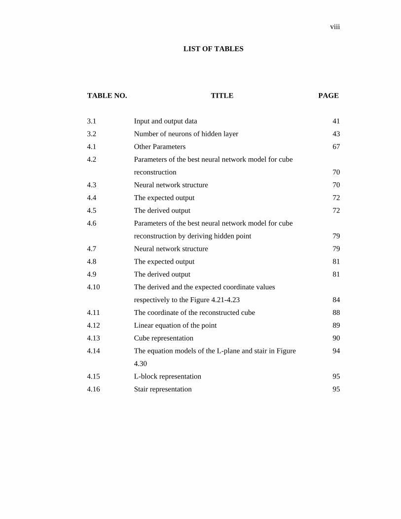
LIST OF TABLES
TABLE NO. TITLE
PAGE
3.1
3.2
4.1
4.2
4.3
4.4
4.5
4.6
4.7
4.8
4.9
4.10
4.11
4.12
4.13
4.14
4.15
4.16
Input and output data
Number of neurons of hidden layer
Other Parameters
Parameters of the best neural network model for cube
reconstruction
Neural network structure
The expected output
The derived output
Parameters of the best neural network model for cube
reconstruction by deriving hidden point
Neural network structure
The expected output
The derived output
The derived and the expected coordinate values
respectively to the Figure 4.21-4.23
The coordinate of the reconstructed cube
Linear equation of the point
Cube representation
The equation models of the L-plane and stair in Figure
4.30
L-block representation
Stair representation
41
43
67
70
70
72
72
79
79
81
81
84
88
89
90
94
95
95
ix
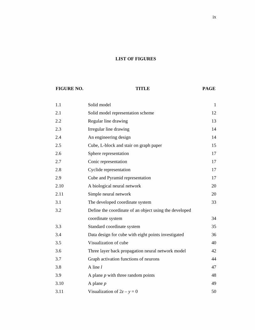
LIST OF FIGURES
FIGURE NO. TITLE
PAGE
1.1
2.1
2.2
2.3
2.4
2.5
2.6
2.7
2.8
2.9
2.10
2.11
3.1
3.2
3.3
3.4
3.5
3.6
3.7
3.8
3.9
3.10
3.11
Solid model
Solid model representation scheme
Regular line drawing
Irregular line drawing
An engineering design
Cube, L-block and stair on graph paper
Sphere representation
Conic representation
Cyclide representation
Cube and Pyramid representation
A biological neural network
Simple neural network
The developed coordinate system
Define the coordinate of an object using the developed
coordinate system
Standard coordinate system
Data design for cube with eight points investigated
Visualization of cube
Three layer back propagation neural network model
Graph activation functions of neurons
A line l
A plane p with three random points
A plane p
Visualization of 2z – y = 0
1
12
13
14
14
15
17
17
17
17
20
20
33
34
35
36
40
42
44
47
48
49
50
x
4.1
4.2
4.3
4.4
4.5
4.6
4.7
4.8
4.9
4.10
4.11
4.12
4.13
4.14
4.15
4.16
4.17
4.18
4.19
4.20
4.21
4.22
4.23
4.24
4.25
4.26
4.27
4.28
4.29
4.30
5.1
The new framework
Generic form of data design
Cube with eight z-values investigated
L-block with twelve z-values investigated
Stair with sixteen z-values investigated
Data design for deriving depth values of cube
Cube with one hidden point
L-block with one hidden point
Stair with one hidden point
Data design for deriving hidden point of L-block
The diagram of the neural network model development
Iteration in MATLAB windows mode
Iteration in graph mode
The reconstructed cube
The reconstructed L-block
The reconstructed stair
The steps of deriving depth values
The diagram steps of the development of neural network
model and the testing process
Iteration in MATLAB windows mode
Iteration in graph mode
Cube reconstruction by deriving hidden point
L-block reconstruction by deriving hidden point
Stair reconstruction by deriving hidden point
The framework of the proposed algorithm
The reconstructed cube
The visualization of the equation models of the
reconstructed cube
Part of the source code
Triangular form
Rectangular form
L-plane and stair visualizations
Schematic of research framework summary
54
56
57
57
58
59
60
61
62
63
69
71
71
73
73
74
74
78
80
80
82
83
83
87
88
91
92
93
93
94
98
1
Bab 1 Pengenalan (Chapter 1 - Introduction):
This chapter presents a brief discussion about the contents of this thesis and explains the
overall topics of the research. It is started with the discussion of solid modeling and definitions that
this research dealt with, issues on that, research motivation, problems, objectives, assumptions,
scopes and limitations. A brief discussion on the contributions of the research and the outline of this
thesis are also included in this chapter.
1.1 Solid Modeling
Solid modeling is a computer description of three-dimensional (3D) objects in sufficient
details to render, analyze, or manufacture the model in realistic manner (Haron, 2004). Huffman
(1971) has investigated research on solid model since early 70’s and the map road to solid modeling
has become one of a valuable field of research until today. Many inventions on that have been used
in the areas of medical imaging and artistic applications, product design, rapid prototyping and
reverse engineering, computer graphics and product visualization.
Solid model represents the solid parts of an object. It is unambiguous representation, which
has the inside and the outside parts that can be sliced open, and it must be correct in representing
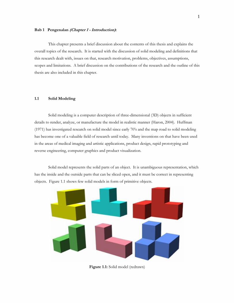
objects. Figure 1.1 shows few solid models in form of primitive objects.
Figure 1.1: Solid model (redrawn)
2
Four related topics related to solid modeling are representation, reconstruction, visualization
and beautification. Solid model representation describes systems, methods, or techniques on how
solid model are represented. The discussion on that can be categorized into four parts, which are
implicit, enumerative, boundary schemes, and deformational schemes (Cretu, 2003). Discussions on
previous works show that constructive solid geometry (CSG), boundary representation (B-rep) and
sweep representations are the most useful techniques of solid model representations.
Solid model reconstruction describes algorithms or methods that are used to reconstruct
uncompleted or unstructured solid model. There are several established methods introduced before.
They are based on mathematical modeling, geometrical analysis, and intelligence approaches that are
usually called as soft computing approach. Recently, method based on intelligence approaches that
used soft computing are much prefer than others. The method avoids the uses of mathematical and
geometrical analysis, which is complicated and difficult to understand.
In conjunction with the reconstruction process, there are two types of 2D line drawing that
are single view and multiple view images, and there are two stages in reconstruction. First, is deriving
depth values of visible points and second is the deriving of hidden point of solid models.
Unfortunately, some of the proposed techniques are not suitable for solid model reconstruction from
single view image. Therefore, to complete the continuation works on solid model reconstruction,
this thesis attempt to devise any technique that deal with solid model reconstruction from given a
single two-dimensional (2D) line drawing.
Visualization means a graphic representation from a set of data. Some techniques will be
appropriate only for specific applications while others are more generic and can be used in many
applications. According to the issues of solid model and the research focus, visualizations techniques
are used to show the representation and the reconstruction of solid model as graphical mode.
Beautification means a process in making of an improvement for visualizations and the reconstructed
object. However, works on visualizations and beautifications are beyond of the scopes of this thesis.
This research focuses the investigation on the reconstruction and the representation of solid model.
3
1.2 Solid Model Reconstruction and Representation
As mentioned earlier, the discussion on solid modeling is categorized into four parts, and
this research deal with two of them, the reconstruction and the representation. In terms of
reconstruction, there are three issues that need to be considered. They are the sources of image or
data, the techniques for reconstruction process, and the techniques for represent an image or
reconstructed object. Techniques in reconstructing solid model object have been developed before.
They are shading, lighting, occlusion, optical flow, line labeling, gradient space, linear system,
primitive identification, minimum standard deviation, analytical heuristic (Lipson and Shpitalni,
1996).
Since in the early time investigated until now, the techniques used for solid model
reconstruction were changed time by time. Modern approaches using soft computing such as
artificial intelligence have replaced some techniques that developed based on mathematical and
geometrical modeling. Barhak and Fischer (2001) explored the adaptive reconstruction of freeform
objects with 3D self-organizing maps (SOM) neural networks grid. Peng and Shamsuddin (2004)
explored the ability of neural networks in learning through experience when reconstructing an object
by estimating its z-coordinate. Fayolle et al. (2004) used genetic algorithms on 3D shape
reconstruction of template models. Junior et al. (2004) used neural networks and adaptive geometry
meshes as a method for surface reconstruction. The technique is very successful in reconstructing
forms with different geometry. Samadzadegan et al. (2005) developed a method based on neuro-
fuzzy modeling for automatic 3D object recognition and reconstruction. Yan Tangy et al. (2007) also
applied neural network with powerful property of approximation to reconstruct complex objects
based on fringe projection.
Based on the previous researches since 1971 to 2007, there are only few researches focused
on solid model reconstruction from single view image of 2D line drawing analysis. Many techniques
have been developed either based on mathematical modeling or artificial intelligence as a modern
approach deal with image from multiple views, or not suitable for 2D line drawing analysis and single
sketch. In 2006, Matondang et al. (2006) used skewed symmetry to derive gradient estimates that
will be used in estimating z-values of 3D object that represented by 2D data. However, the
experimental results of this work show a lot of weaknesses in using skewed symmetry to estimates z-
values. So far, there are no works that attempt to devise any technique for solid model
reconstruction from given 2D line drawing using artificial intelligence approaches. Based on these
4
facts, this thesis focuses the investigation on solid model reconstruction from given 2D line drawing
as the source of image based on the uses of artificial intelligence approach.
In terms of solid model representation, several established techniques have been introduced
before. Piperakis et al. (2001) has introduced some of the common and important methods of
representation. First is approximated by a net mesh or planar polygonal facets that used for
polygonal objects representation. Second is bi-cubic parametric patches that used for curved surface
of polygonal objects representation. It is called curve quadrilaterals. Third is constructive solid
geometry (CSG) which is another method of exact representation for solid model representation.
Spatial subdivision techniques such as voxel also used for solid model representation. These
techniques dividing the object space into elementary cubes. Another two types of representation are
implicit and explicit function. These techniques used mathematical models in representing solid
model, such as, 2 2 2x y r+ = which is the representation of a sphere and
2 2 2 2 2 2 2 2 2( ) 4 ( )x y z R r R x y+ + + − = + which is the torus representation. Based on discussion
of previous works, the most techniques used are CSG, B-rep and sweep representation. Cretu et al.
(2003) has introduced the neural network structure architecture for 3D object representation. In
2004, Peng and Shamsuddin (2004) used neural network in representing 3D objects from polygonal
type to neural network representation. So far there are no researches and reports that developed the
uses of mathematical models in representing solid model besides the established ones. Therefore,
this research tries to develop a new algorithm using mathematical models in representing solid model
based on surface based model. This approach is similar with explicit and implicit function
representation. The experimental result shows that the algorithm has the advantages and the
disadvantages in representing solid models.
1.3 Problem Statement
Based on the discussion above, there are several reports of techniques used for object
reconstruction from multiple views by matching between different views. These approaches are not
suitable for analysis of a single sketch. Therefore, the main question is: Is it possible to develop a
technique for solid model reconstruction from given 2D line drawing?
5
Besides that many techniques have been introduced and developed for object reconstruction
from multiple view images are based on exact techniques such as mathematical modeling geometrical
analysis. There just few research employed the ability of artificial intelligence approaches or others
soft computing. Even if there are several reports used artificial intelligence techniques for 3D object;
they are not suitable for solid model from given 2D line drawing. The problem is: Is it possible to
develop an artificial intelligence technique to reconstruct solid model from given 2D line drawing,
such as neural network or fuzzy system?
However, these facts gives motivation for this research to answer and solve the problem:
Why there are no researches, which are conducted the three terms of reconstruction, namely the 3D
object (in case of solid modeling), the source of image (2D line drawing), and the techniques
(artificial intelligence approach)?
Besides these issues and motivation, in terms of solid model representation, the author also
found that there are no works employed mathematical models in representing solid models based on
surface based-model. Since that, this research also tries to face and answers if there are any
possibility to represent solid model as mathematical models. This kind of representation also called
as parametric models that used implicit or explicit function representations.
1.4 Objectives
Based on the discussion and the problem statement, this thesis focuses the investigation on
the reconstruction and the representation of solid model from given 2D line drawing. Four stages
involved are data preparation, reconstruction process, representation process and visualization for
validating purpose. Based on these stages, the objective of this research can be divided into four
objectives as follows:
1. To develop a new framework in reconstructing and representing solid model.
2. To develop neural network models in reconstructing solid model by deriving the
depth values and deriving hidden point.
6
3. To develop a new experimental data design to be used in the development process of
neural network models.
4. To develop a hybrid-computing algorithm based on the uses of neural network and
mathematical modeling in representing solid model.
1.5 Scope and Limitation
As mentioned earlier in Section 1.2, this thesis focuses the investigation on the solid models
that is represented by given 2D line drawing. The 2D line drawing used is a valid line drawing of
engineering sketch that represent solid model. Otherwise line drawing of impossible object,
wireframe object, origami world is not accepted.
Three solid models are used in this research as the input to develop and test neural network
models and the proposed algorithm. They are cube, L-block and stair. A cube has eight points in
form of ( , , )x y z , twelve lines and six planes. A L-block has twelve points in form of ( , , )x y z ,
eighteen lines and eight planes. A stair has sixteen points in form of ( , , )x y z , twenty two lines and
ten planes. The solid model are drawn on graph paper and the values of ( , , )x y z are defined.
In reconstructing solid model, neural network with back propagation are applied and been
developed to derive depth values and hidden point of solid model. Therefore, the process is divided
into two cases. First case is reconstruction by deriving depth values of solid model where all the
points ( ( , )x y values) are known. In this case, the depth values are derived. Second case is
reconstruction by deriving hidden point (invisible point) of solid model where all the points
( ( , )x y values) are known, except the hidden one. In this case, the hidden point is derived. However,
these two approaches are capable in reconstructing solid model from given 2D line drawing.
In representing solid model, an algorithm which is a hybrid system between neural network
and mathematical modeling are developed. Once the solid models are reconstructed used neural
network models, and then mathematical models applied to represent the solid model based on
7
surface based model as equations models. This kind of representation usually used explicit and
implicit functions. The analyses to the contributions of the research are present by creating direct
comparison to the expected results and few results of previous works.
1.6 Assumptions
There are few assumptions that have been made to simplify the implementation of this
research work and the contributions. First, the solid models tested are assumed as an engineering
sketch in the form of 2D line drawing that represent solid model on graph paper. Second, the 2D
line drawing is assumed to represent a valid solid model where all unwanted points or lines have been
removed and there are no unconnected points or lines. Third, the solid model is assumed as a 2D
line drawing with all informative lines shown. Fourth, there is only one hidden point in the backside
of the solid model. Fifth, this research assumed that the ( , , )x y z values of solid models are known.
These assumptions make the proposed algorithms more logical or otherwise the engineering sketch is
not seen as solid models because the projection is parallel to the other faces of the object. In this
case, it is impossible to interpret, reconstruct and represent the sketches as solid model and hence the
analysis of the accuracy of the results simpler.
1.7 Research Contribution
This thesis has four main results as the research contributions. They are the framework for
solid model reconstruction and representation, the developed neural network models in
reconstructing solid model from given 2D line drawing, the developed experimental data design, and
a hybrid computing algorithm in representing solid model. An artificial intelligence technique, neural
network and mathematical modeling are two approaches that are involved to solve the problems of
the research and achieve all the objectives
The framework for solid model reconstruction and representation is yielded based on three
main parts, namely the data preparation and definition which involved to the uses of graph paper and
8
affine transformation, neural network toolbox in MATLAB 7.14, and mathematical modeling. The
framework covered the representation process as continuation works of the reconstruction process.
Neural network models are developed in this research. The development process employed
back propagation algorithm as the learning rule then the best neural network model used to derive
depth values and hidden point of solid model. Therefore, the reconstruction process is categorized
into two parts and they are developed separately. Solid models from given 2D line drawing in form
of engineering sketch are used as the inputs on the development process and to test the models.
In conjunction with the development of neural network models, another contribution of the
research is also presented in this thesis. It is a new experimental data design that is used in training,
validating and testing stages of neural network model development. Generally, the data are designed
based on moving average method, where the input data and the output data are arranged in a row.
However, in this research the input and the output data are designed in a column. This is to make
sure the developed network model give a satisfactory result then another one.
A hybrid computing algorithm in representing solid model also developed in this research.
This contribution is a continuing stage of the solid model reconstruction. In this algorithm, two
approaches were conducted to represent solid model. They are neural network with back
propagation and mathematical modeling. The input was taken from given engineering sketch of 2D
line drawing and employed neural network to reconstruct the solid model by deriving the depth
values. Once the depth values derived, then mathematical modeling employed to represent the solid,
based on surface based model in form of mathematical models (equation models).
In case of representing the solid model as equation models, two techniques could be used namely
Determinant Rule and Gauss Jordan method to generate the models. MATLAB 7.14 was used in
this research to facilitate the overall requirements of the research, mainly for calculations, validations,
visualization, and neural network models development. The experimental results show that the
proposed neural network models and the proposed algorithm are capable and successfully in
reconstructing solid model and representing the reconstructed solid.
9
Bab 2 Kajian Literatur (Chapter 2 - Literature Study):
This chapter presents literatures that related to the research topic and discussion on few
previous works on solid model reconstruction and representation. The discussions are divided into
nine sections. Section 2.1 generally discusses about model or modeling, and followed by Section 2.2,
which discuss about solid model and its issues. Section 2.3 presents a brief discussion of line
drawing, which used as the source of the data for the developed research, and followed by Section
2.4, which presents a discussion on geometrical modeling and introduction to mathematical model,
which used parametric models to represent a solid model. Discussion on neural network as soft
computing techniques is presented in Section 2.5, and then followed by Section 2.6 and 2.7 which
present discussion of previous works on solid model reconstruction and representation. The
discussion of this chapter ends up with Section 2.8 and 2.9, which present the research focus and a
summary of this chapter.
2.1 Model or Modeling
Models or modeling may refer to a pattern, plan, representation, or description design to
show the structure or working of an object, system, or concept. They are giving an easy
understanding of how the objects are working rather than just describes by words. The closet
definition of model or modeling to the context of three-dimensional (3D) graphics can be expressed
as the process of giving schematic description of the object that composes a scene (Cretu, 2003).
There are six criteria that give a good contribution to the final-result when building an object model.
They are the methods to acquire or create the data that describes the object, the purpose of the
model, the implementation complexity, its computational, its conformance, and the ease of model
manipulation (Cretu, 2003).
Based on how to represent a model, the discussion on modeling system is divided into four
parts, namely wire frame model, surface model, solid model, and procedural model (Foley et al.
1996). A wire frame model is a visual presentation of an electronic representation of a 3D or
physical object used in 3D computer graphics. It is created by specifying each edge of the object
where two mathematically continuous smooth surfaces meet, or by connecting an object’s
10
component vertices using straight lines or curves. Wire frame model allows visualization of the
underlying design structure of a 3D model.
Surface model describes process of representing a physical or artificial created surface by
means of mathematical expression, such as mathematical model of sphere 2 2 2 2( )x y z r+ + = ,
right circular cylinder 2 2( 4 12 0)x y x+ − − = , ellipsoid 22 2
2 2 2( 1)yx za b c+ + = , and a plane of a cube
( 0)ax by cz d+ + + = . Surface modeling is widely used in 3D animation for games and other
presentation. Surface modeling is more complex method for representing objects compared than
wire frame modeling.
Solid model is the unambiguous representation of the solid parts of an object. It is quite
different with a surface model, although they appear the same on screen. Solid model can be sliced
open but not with surface model. In surface modeling, object can be geometrically incorrect,
whereas it must be correct with solid modeling. Models of solid objects are suitable for computer
processing.
As a special case on modeling system, procedural model are generative processes that
describe objects that can interact with external even to modify themselves (Foley et al., 1996). Each
procedural model of a 3D object is described in terms of components and a procedure (algorithm)
that shows how to generate the object and how to control its shape using these components. The
most common procedural models are fractals, graftals, and particle system.
However, research on models or modeling systems is a wide field of research. The author of
this thesis decided to focuses the investigation and the work on solid models and their issues. The
research is focused to the reconstruction and the representation of solid model. Next section
presents a brief discussions and issues on that.
2.2 Solid Model and Issues
Solid model describes the volumes of space occupied by solid parts. It differs from surface
model in several ways. Solid model, unlike surface, contains its boundary. While it is possible to
11
decompose a solid object into smaller patches, it is not possible to convert a surface into a real 3D
object. Moreover, unlike surface, a solid model has an inside and outside (Cretu, 2003).
The development of solid modeler involves visualization technology for the viewing and
manipulating of solid models, technical drawing and other related documentation of manufactured
components and large assemblies of products. Sutherland (1963) started the research on software
development of solid modeler. His evolution on CAD has been successfully replace the uses of
pencils and papers as common tools and also light pen and digitizer which are use to sketch by
engineers. Furthermore, his evolution on CAD system had given tremendous effect on the
development of CAD software. Since then, the required of CAD software in designing, updating,
storing, and visualizing engineering drawing have rapidly improved. However, in this research none
of the establish software discuss earlier are used or involved. The discussions are focused more on
the uses of soft and hard computing to enhance solid modeler for reconstruction and representation
of solid model. In case of solid model reconstruction, the discussion could be categorized into three
parts. They are the sources of image, the techniques for solid model reconstruction, and the
techniques for representing reconstructed solid model.
Heyden (1995), introduced five different cases that need to be considered in 3D
reconstruction as a source of images or data that have been reconstructed. The first is an image
taken with un-calibrated camera, making it possible to reconstruct the object up to projective
transformations; the second is an image reconstruct from calibrated camera, making it possible to
reconstruct the object up to similar transformations. The third case is in the form of algebraic
properties of the multi-linear functions, and the ideals generated by them. The fourth is Euclidean
reconstruction technique when some information of the calibrated camera are given; and the last case
is reconstruction of one image of an object or line drawing, which is known to be piecewise planar.
Many techniques for solid model reconstruction introduced in the last several decades are
related to mathematical modeling. They are the gradient space, the linear systems approach, the
interactive method, perceptual approach, the minimum standard deviation, analytical heuristic, the
primitive identification, and line labeling. However, the uses of mathematical models and
geometrical analyses made the techniques complicated and difficult to understand. In the mean time,
techniques that are related to artificial intelligence have become a new approach in the area of solid
reconstruction. The uses of neural network (such as Barhak and Fischer, 2001), fuzzy logic (such as
12
Samadzadegan et al., 2005), and genetic algorithm (such as Fayolle et al., 2004) have to be a new
significant approach on solid model reconstruction.
Unfortunately, the discussions on previous works lead to the conclusion that many
researches have been developed do not take line drawing as the sources of image. Most of the
techniques or methods introduced before are used to reconstruct 3D object from multiple views
image and matching features between different views and for sure they are not suitable for analysis of
a single sketch. Details discussions on these issues given in Section 2.6.
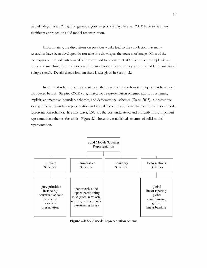
In terms of solid model representation, there are few methods or techniques that have been
introduced before. Shapiro (2002) categorized solid representation schemes into four schemes;
implicit, enumerative, boundary schemes, and deformational schemes (Cretu, 2003). Constructive
solid geometry, boundary representation and spatial decompositions are the most uses of solid model
representation schemes. In some cases, CSG are the best understood and currently most important
representation schemes for solids. Figure 2.1 shows the established schemes of solid model
representation.
Figure 2.1: Solid model representation scheme
13
2.3 Line Drawing
Line drawing is one of the simplest techniques uses for graphic interpretation in many areas.
It represents 2D scenes such as diagram and plans and 3D scenes such as solid model or origami
word (Haron, 2004). This section discusses source of line drawing which is used as the pre-input of
the research.
2.3.1 Introduction to Line Drawing
A line drawing is an abstraction derived from an image that conveys its information solely
through the shape of thin lines on a contrasting background. The discussion on line drawing is
divided into regular and irregular (Freeman, 1969). With the help of computer aided design (CAD)
system, irregular line drawing can be improved by using the editing command. Unfortunately this
system eliminates the naturalness of the sketching.
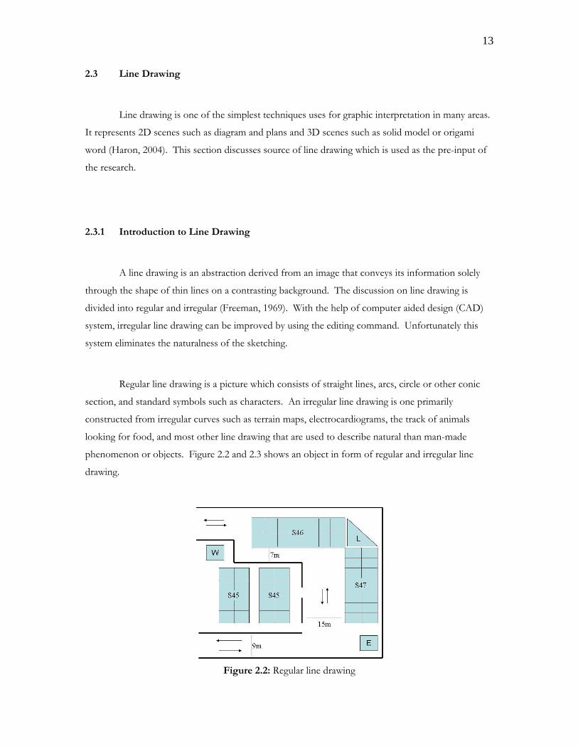
Regular line drawing is a picture which consists of straight lines, arcs, circle or other conic
section, and standard symbols such as characters. An irregular line drawing is one primarily
constructed from irregular curves such as terrain maps, electrocardiograms, the track of animals
looking for food, and most other line drawing that are used to describe natural than man-made
phenomenon or objects. Figure 2.2 and 2.3 shows an object in form of regular and irregular line
drawing.
Figure 2.2: Regular line drawing
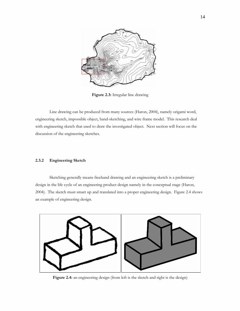
14
Figure 2.3: Irregular line drawing
Line drawing can be produced from many sources (Haron, 2004), namely origami word,
engineering sketch, impossible object, hand-sketching, and wire frame model. This research deal
with engineering sketch that used to draw the investigated object. Next section will focus on the
discussion of the engineering sketches.
2.3.2 Engineering Sketch
Sketching generally means freehand drawing and an engineering sketch is a preliminary
design in the life cycle of an engineering product design namely in the conceptual stage (Haron,
2004). The sketch must smart up and translated into a proper engineering design. Figure 2.4 shows
an example of engineering design.
Figure 2.4: an engineering design (from left is the sketch and right is the design)
15
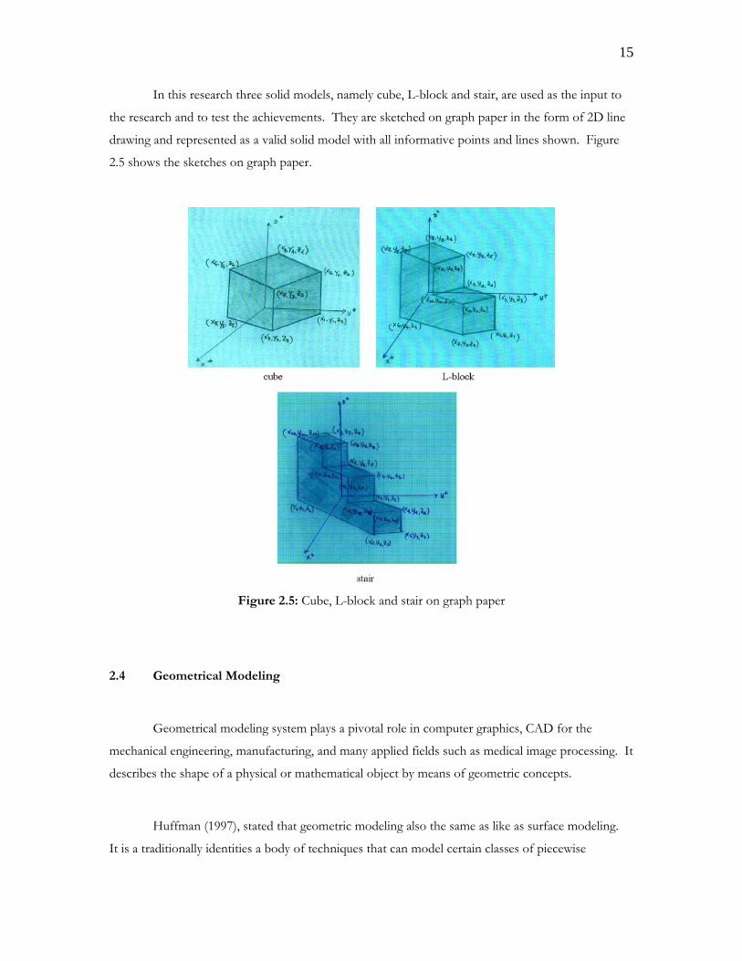
In this research three solid models, namely cube, L-block and stair, are used as the input to
the research and to test the achievements. They are sketched on graph paper in the form of 2D line
drawing and represented as a valid solid model with all informative points and lines shown. Figure
2.5 shows the sketches on graph paper.
Figure 2.5: Cube, L-block and stair on graph paper
2.4 Geometrical Modeling
Geometrical modeling system plays a pivotal role in computer graphics, CAD for the
mechanical engineering, manufacturing, and many applied fields such as medical image processing. It
describes the shape of a physical or mathematical object by means of geometric concepts.
Huffman (1997), stated that geometric modeling also the same as like as surface modeling.
It is a traditionally identities a body of techniques that can model certain classes of piecewise
16
parametric surfaces, subject to particular conditions of shape and smoothness. It is developed as a
separate field in several industries, including automobile, aerospace, and shipbuilding, and has some
of its intellectual roots in approximation theory.
Geometric models can be built for objects of any dimension in any geometric space. Both
2D and 3D geometric models are extensively used in computer graphics. Geometric models are
usually distinguished from procedural and object-oriented models, which define the shape implicitly
by the specific algorithm. They are also contrasted with digital images and volumetric models; and
with implicit mathematical models such as the zero set of an arbitrary polynomial. However, the
distinction is often blurred: for instance, geometric shapes can be represented by objects; a digital
image can be interpreted as a collection of colored squares; and geometric shapes such as circles are
defined by implicit mathematical equations. Also, the modeling of fractal objects often requires a
combination of geometric and procedural techniques. In this research, the geometric shapes of solid
models are defined by implicit mathematical equations or mathematical models. Next subsection
presents a brief discussion on mathematical model.
2.4.1 Mathematical Model
Mathematical model is a conceptual model that uses mathematical languages rather than
ordinary languages to represent a particular scientific context. The scientific context itself would
ordinarily be one that exists in the real world and the model is necessarily a simplified description of
the actual context (Bross, 1972). As an abstract model, mathematical model uses mathematical
language to describe the behavior of a system. It can take many forms, including but not limited to
dynamical systems, statistical models, different equations, or game theoretic models. Eykhoff (1974)
defines a mathematical model as ‘a representation of the essential aspects of an existing system (or a
system to be constructed) which presents knowledge of that system in usable form’.
In case of solid model representation, mathematical models can be used to represent the
geometrical shape of solid models, which are the outer parts of the model. In other words,
mathematical models can be used to represent solid models based on surface based-model.
17
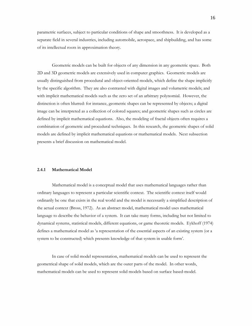
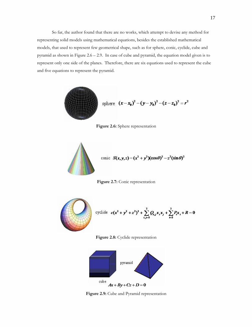
So far, the author found that there are no works, which attempt to devise any method for
representing solid models using mathematical equations, besides the established mathematical
models, that used to represent few geometrical shape, such as for sphere, conic, cyclide, cube and
pyramid as shown in Figure 2.6 – 2.9. In case of cube and pyramid, the equation model given is to
represent only one side of the planes. Therefore, there are six equations used to represent the cube
and five equations to represent the pyramid.
Figure 2.6: Sphere representation
Figure 2.7: Conic representation
Figure 2.8: Cyclide representation
Figure 2.9: Cube and Pyramid representation
18
2.5 Neural Network
This section presents a discussion on neural network as an approach that being developed in
this research. Neural network is one of the artificial intelligence techniques that also known as soft
computing technique. It is like a machine learning that has the ability to recognize or analyze a
system or data with learns by examples. The discussion started with a brief introduction of soft
computing.
2.5.1 Introduction to Soft Computing
Generally, there are two kinds of computing techniques; soft and hard computing. Soft
Computing is the fusion of methodologies that were designed to model and enable solutions to real
world problems, which are not modeled, or too difficult to model, mathematically (Moussa, 2003).
Meanwhile, hard computing is defined as the antipode of soft computing, such as a heterogeneous
collection of traditional computing methods. Hard computing schemes strive for exactness and full
truth, while soft computing is an emerging collection of methodologies, which aim to exploit
tolerance for imprecision, uncertainty, and partial truth to achieve robustness, tractability, and low
total cost (Ovaska et al., 1999). This is the case when soft computing is utilized for complementing
the performance of traditional hard computing algorithms, or even replacing them. However, in this
research both of them, soft and hard computing are used.
The main goal of soft computing is to develop intelligent machines and to solve nonlinear
and mathematically un-modeled system problems (Zadeh 1993, 1996, and 1999). The applications of
Soft Computing have proved two main advantages. First, it made solving nonlinear problems, in
which mathematical (hard computing) models are not available, possible. Second, it introduced the
human knowledge such as cognition, recognition, understanding, learning, and others into the fields
of computing.
Whether soft computing (SC) and hard computing (HC) methodologies are fused together
successfully in numerous industrial applications, soft computing is hidden inside the system or
subsystem, and the end user does not necessarily know that soft computing are being used for
control, fault diagnosis and pattern recognition (Ovaska, 2006). Fuzzy Logic (FL), Neural Network
19
(NN) and Genetic Algorithm (GA) are the core methodologies of soft computing. They are part of
artificial intelligence.
2.5.2 Introduction to Neural Network
Neural network is an information-processing paradigm that is inspired by the way biological
neurons system, such as the brain, process information (Christos and Dimitrios, 1996). It is
composed of a large number of highly interconnected processing elements (neurons) working in
unison to solve specific problems. As like as people, a neural network learns by example. A neural
network configured for a specific application, pattern recognition or data classification, trough a
learning process.
Neural networks have been applied to an increasing number of real-world problems of
considerable complexity. Their most important advantages are to solve problems that are too
complex for conventional technologies, problem that do not have an algorithm solution or for which
an algorithm solution is too complex to be found. Neural networks are well suited to problems that
people are good at solving, but for which computers are not. These problems included pattern
recognition and forecasting (which requires the recognition of trends in data).
In biological area, a neural network can be defined as a model of reasoning based on the
human brain. The brain consists of densely interconnected set of nerve cells, or basic-information-
processing units, called neurons. The human brain incorporates nearly 10 billion neurons and 60
trillions connections, synapses, between them (Shepherd and Koch, 1990). By using multiple
neurons simultaneously, the brain can perform its functions much faster than the fastest computers
in existence today. A neuron consists of a cell body (soma), a number of fibres (dendrites), and a
single long fibre (axon). While dendrites branch into a network around the soma, the axon stretches
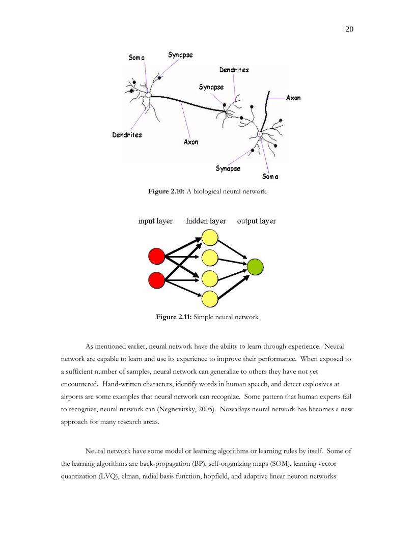
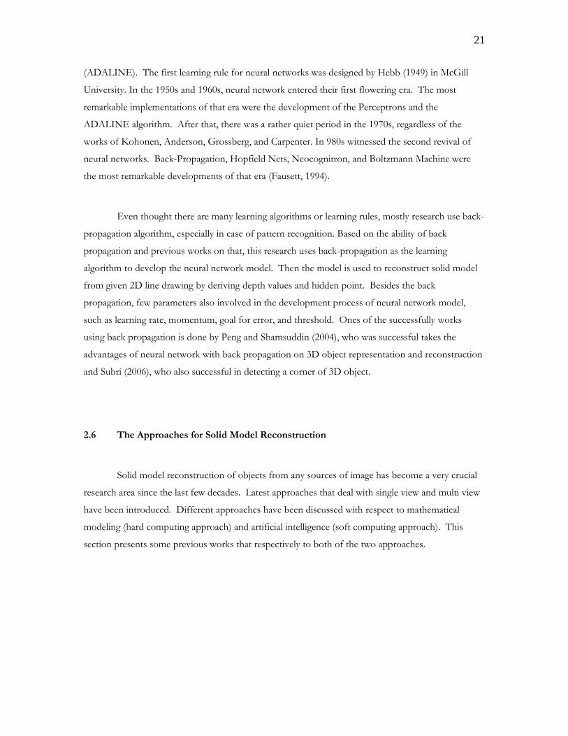
out to the dendrites and somas of other neurons. Figure 2.10 shows the schematic drawing of a
biological neural network, and followed by Figure 2.11 shows a simple architecture of a neural
network.
20
Figure 2.10: A biological neural network
Figure 2.11: Simple neural network
As mentioned earlier, neural network have the ability to learn through experience. Neural
network are capable to learn and use its experience to improve their performance. When exposed to
a sufficient number of samples, neural network can generalize to others they have not yet
encountered. Hand-written characters, identify words in human speech, and detect explosives at
airports are some examples that neural network can recognize. Some pattern that human experts fail
to recognize, neural network can (Negnevitsky, 2005). Nowadays neural network has becomes a new
approach for many research areas.
Neural network have some model or learning algorithms or learning rules by itself. Some of
the learning algorithms are back-propagation (BP), self-organizing maps (SOM), learning vector
quantization (LVQ), elman, radial basis function, hopfield, and adaptive linear neuron networks
21
(ADALINE). The first learning rule for neural networks was designed by Hebb (1949) in McGill
University. In the 1950s and 1960s, neural network entered their first flowering era. The most
remarkable implementations of that era were the development of the Perceptrons and the
ADALINE algorithm. After that, there was a rather quiet period in the 1970s, regardless of the
works of Kohonen, Anderson, Grossberg, and Carpenter. In 980s witnessed the second revival of
neural networks. Back-Propagation, Hopfield Nets, Neocognitron, and Boltzmann Machine were
the most remarkable developments of that era (Fausett, 1994).
Even thought there are many learning algorithms or learning rules, mostly research use back-
propagation algorithm, especially in case of pattern recognition. Based on the ability of back
propagation and previous works on that, this research uses back-propagation as the learning
algorithm to develop the neural network model. Then the model is used to reconstruct solid model
from given 2D line drawing by deriving depth values and hidden point. Besides the back
propagation, few parameters also involved in the development process of neural network model,
such as learning rate, momentum, goal for error, and threshold. Ones of the successfully works
using back propagation is done by Peng and Shamsuddin (2004), who was successful takes the
advantages of neural network with back propagation on 3D object representation and reconstruction
and Subri (2006), who also successful in detecting a corner of 3D object.
2.6 The Approaches for Solid Model Reconstruction
Solid model reconstruction of objects from any sources of image has become a very crucial
research area since the last few decades. Latest approaches that deal with single view and multi view
have been introduced. Different approaches have been discussed with respect to mathematical
modeling (hard computing approach) and artificial intelligence (soft computing approach). This
section presents some previous works that respectively to both of the two approaches.
22
2.6.1 Mathematical and Geometrical Modeling Approach
Research in solid modeling started with a few exploratory efforts in mid-1960s, but begins in
earnest in the early 1970s, when several research groups were established in the main industrial
nations (Reguicha and Rossignac, 1992). Solid modeling’s mathematical foundations come primarily
from topology and algebraic geometry. The discussion can be classified into two categorized. They
are single view approach and multiple view approach (Wang, 1992). The single view approach
includes mainly line labeling scheme, gradient space method, linear programming and perceptual
algorithm (Wang, 1993), interactive methods, the primitive identification, the minimum standard
deviation, and analytical heuristics (Lipson and Shpitalni, 1996). The multiple view approach
includes the Boundary representation (B-rep), the Constructive Solid Geometry (CSG) and Logical
Representation (LR). The following discussion introduces the single view approaches.
Line labeling is a form of interpreting a line drawing; it provides spatial information about
the scene but does not yield an explicit 3D representation. Each line in the drawing is assigned one
of three meanings: convex “+” (ridge), concave “−” (corner of a room), or occluding edge “→”,
where the direction of the arrow marks the side of occlusion. Junction dictionaries and constraint
graphs are used to find consistent assignments (Huffman, 1971; Clowes, 1971).
The gradient space approach draws a relationship between the slope of line in the drawing
plane and the gradient of faces in the depicted 3D scene. Assuming a particular type of projection, an
exact mathematical relationship can be computed, and possible interpretations of the drawing can be
constrained (Mackworth, 1973; Wei, 1987). Like labeling approach, this approach also gives a
necessary but not sufficient condition for a sketch to be recognizable.
The linear system approach uses a set of linear equalities and inequalities defined in terms of
the vertex coordinate and plane equations of object faces, determined by whether vertices are on, in
front of or behind the polygon faces. The solvability of this linear program is a sufficient condition
for the reconstruct ability of the object (Sugihara, 1986; Grimstead and Martin, 1995). Linear
programming optimization may yield a solution.
23
Interactive methods gradually build up the 3D structure by attaching facets one after the
other as sketch and specified by a user. The aim is to provide a practical method for constructing 3D
models in an interactive CAD/CAM environment (Fukui, 1988; Lamb and Bandopadhay, 1990).
Perceptual Approach systems generally tend to carry out 3D reconstruction based on set of
heuristic rules rather than on extensive numerical calculations (Idesawa, 1973). Lamb and
Bandopadhay (1990) was developed a system which took a single axonometric hidden lines removed
sketch as user input. This sketch creates an adjacency graph of all the vertices and additional
information, such as slope and length of the lines. Then, the graph is label to reject impossible
objects and to determine the hidden face information. Moreover, the best line junction in the
drawing is assumed to be the origin. This algorithm assumes that a best line junction exist, which may
not be true in all drawings. The major advantage of this method is because of its heuristic nature that
can tolerate in accuracies in the input.
The primitive identification approach reconstructs the scene by recognizing instances or
partial instances of known primitive shapes, such as blocks, cylinders, etc. This approach contains a
strict assumption that the depicted 3D object is composed entirely of known primitives, but has the
benefit of yielding the final 3D structure in a convenient constructive solid geometry (CSG) form (e.g.
Wang and Grinstein, 1989).
The minimum standard deviation approach focuses on a single and simple observation; that
human interpretation of line drawing tends towards the most ‘simple’ interpretation. Marill (1991)
defined simplicity as an interpretation in which angel created between lines and at junctions are as
uniform as possible across the reconstructed object, inflating the flat sketch into a regularized 3D
object (Leclerc and Fiscler, 1992). Although Marill’s algorithm cannot be directly used for the
reconstruction from perspective views, Turner et al (2000) have used a modified version for the
reconstruction of perspective sketches (Wani, 2004).
Analytical Heuristic approaches use coded soft geometrical constraint such as parallelism,
skewed symmetry, and others to seek the most plausible reconstruction (Kanade, 1980; Lipson and
Shpitalni, 1996). Matondang et al. (2006) used skewed symmetry to reconstruct 3D object by
deriving gradient estimates. Moreover, the gradient estimates used to estimates the depth values.
24
Correlation Based Approach is a technique, which is based on the way humans interpret 2D
sketches (Lipson and Sphitalni, 1996). It is similar to a machine learning approach in which a system
learns to correlation between 2D and 3D geometry by creating correlation tables. The system gets
probabilistic analysis of the scene and then the 3D object is reconstructed by using various
reconstruction methods. Some of the correlations exploited are; there is a strong correlation between
vertical lines in a 2D sketch and vertical edge in the real world. They are the angels between two
lines in the sketch, which are strongly correlated to the angels between the same lines in space.
Parallel lines in 2D tend to be parallel in 3D; there is also a strong correlation between the 3D
volume spanned by a corner of three lines and the angels between their projected lines, especially
true of rectangular corners. Then this correlation will be formalized as geometric relationships
between various entities. The reconstruction process is treated as an optimization problem of the
assignment of z-coordinate to maximize the correlation score.
Few previous works discuss above shows that mathematical and geometrical modeling are
capable and have its own ability in reconstructing solid model from given single view image.
However, few disadvantages in terms of the difficulty in using the methods and the analysis was
motivated the author of this thesis to find and develop another method that can be used simpler and
easy to understand. Next section presents few approaches that related to artificial intelligence
techniques.
2.6.2 Artificial Intelligence Approaches
As mentioned earlier, there are some disadvantages in using the techniques which are related
to mathematical and geometrical modeling. Most of them are very complicated with the
mathematical analysis and the geometrical problems. However, the uses of artificial intelligence
approaches for solid model reconstruction since few years ago have given a new tremendous solution
to avoid the uses of the mathematical and geometrical model. Some of them are:
Barhak and Fischer (2001) proposed a neural network self organizing map (SOM) method
for reconstructing a single B-Spline surface from a single image. The Stages of the proposed
reconstruction method are: constructing a parametric grid, parameterize the sample data according to
the parametric grid, creating an initial parametric 3D base surface, projecting the sampled points into
25
3D base surface and correcting their parameterization, approximating a B-Spline surface to the 3D
digitized points, adaptively optimizing the parametric surface by repeating Stage 4-5 until the surface
approximation error satisfies a given convergence tolerance. As a result of applying the proposed
parametric and fitting SOM method, the reconstruction process is highly improved.
Peng and Shamsuddin (2004) integrated an adaptive artificial neural network (ANN) based
method in reconstructing and representing 3D object. The stages of the proposed reconstruction
method are: data acquisition, neural network reconstruction, neural network 3D object
representation, display and affined transformation of object, and compare with original object. The
results show that neural network is a promising approach for reconstruction and representation of a
3D object.
Fayolle et al. (2004) proposed a method, which enable to fit a 3D object defined a functional
representation (FRep) to a dataset of 3D points on its surface. A parametric FRep model sketching
the point-set is fitted to the point-set. The best fitted parameters of the model are obtained by using
genetic algorithm. The efficiency of the approach is illustrated for reverse engineering applications.
Junior et al. (2004) proposed a multi-resolution surface reconstruction method from point
clouds in 3D space based on Kohenen’s self organizing neural networks. The proposed algorithm is
able to create 3D meshes with varieties geometry, in a multi-resolution fashion.
Samadzadegan et al. (2005) developed a method based on neuro-fuzzy modeling for
automatic 3D object recognition and reconstruction. The recognition process could identify 49 of
the 57 objects in their test, which is a quota 86%. The 3D reconstruction of the recognized objects is
well suited for virtual city modeling or 3D GIS object extraction.
Yan Tangy et al. (2007) used neural network with powerful property of approximation to get
the continuous approximate function of a discrete fringe pattern captured by an image grabber. By
dealing with the approximate function the depth-related phase of the measured object modulated
into the fringe pattern can be demodulated. As the results the proposed method successfully to
reconstruct complex objects based on fringe projection and has higher spatial resolution compared
with Fourier Transform Profilometry (FTP).
26
Based on the discussion of the few previous works, it shows that there are very few research
used artificial intelligence techniques in reconstructing solid model from given single view image.
However the uses of artificial intelligence techniques are simpler than method related to
mathematical and geometrical modeling. Therefore, this research attempts to devise an artificial
technique, namely neural network that can be used to reconstruct solid model from given single view
image in the form of 2D line drawing.
2.7 The Approaches for Solid Model Representation
This section presents few methods and previous works that have been used to represent
solid model. The discussion starts with the solid model representation schemes that introduced
before by Shapiro (2002). Figure 2.1 in Section 2.2 shows the diagram of the schemes.
Implicit representations give rules for testing whether the points belong to an object or not.
The most important representations comprised in this category are the pure primitive instancing
schemes, Constructive Solid Geometry (CSG), and sweep representations.
Enumerative representations are also used as a direct way to define whether the points
belong to the solid model or not. There are two approaches that can be used, namely parametric
solids and space-partitioning solids.
Boundary representations are one of another way to describe or represent a solid object by
describing the surface that covers its object. Boundary models are complete representation of a solid
as an organized collection of surfaces. The solid is thus a union of faces (surfaces), bounded by
edges (curves), which in turn are bounded by vertices (points) (Mortenson, 1997).
A deformational scheme is a representations scheme that can be seen as an extension of
affine transformations and set operations for solid object modeling (Cretu, 2003). It is divided into
two categories of deformations. A locally specified deformation modifies only a set of points
corresponding to a sub-region of the object surface (the tangent space of the solid is modified (Barr,
1984)). A globally specified deformation, in contrast, affects an object as a whole, by explicitly
modifying the global coordinates of all solid’s points in space. There are three transformations
27
include global tapering, global twisting, and global bending (Cretu, 2003). Deformation can also be
combined in the form of hierarchical structure. Thus they increase the range and complexity of
solids that can be modeled.
However, based on the discussion on the previous works, the most common schemes for
representing solid modeling are constructive solid geometry (CSG), boundary representation (B-rep),
and spatial decompositions. In some cases, CSG are the best understood and currently most
important representation schemes for solid models. CSG is a direct and effective method to
construct a solid object model. Each object is considered a collection of primitives (primitives are
well defined as a simple solid such as cubes, pyramids, cylinders, cones, and sphere), a set of
transformations (transformation are including translation, rotation, and scaling that are used to define
the position, orientation, and arbitrary the shape of the primitives), and Boolean operations (union,
intersection, and difference that are regularize set operation which can be used as a combining
operators to generate higher level objects). The result of this representation is called CSG-tree,
where leaves are primitives and internal nodes are regularized Boolean operation with
transformation. Meanwhile the desired object is became the root of CSG tree. This method is
conceptually close to engineering practice for designing mechanical parts and architectural details.
A representation of a solid in a spatial occupancy enumeration scheme is essentially a list of
spatial cells occupied by the solid (Reguicha, 1980). The cells, sometimes called voxel (volume
elements), are cubes of a fixed size and lie in a fixed spatial grid. Spatial arrays are unambiguous,
unique (except for positional non-uniqueness), and easy to validate, but they are potentially quite
verbose. Thus spatial arrays may be reasonable representation in certain architectural applications
where buildings are sufficiently modular or in tomography where irregular biological objects are
modeled approximately by polyhedral. Spatial subdivision decomposes a solid into cells, each with a
simple topological structure and often also with a simple geometric structure. Rossignac and
Reguicha (1999) was introduced spatial decomposition into two parts discussion. The first is regular
decompositions. Regular decomposition approximate solids by stacks of constant-thickness slices,
by prismatic columns of square cross-sections and parallel axes, or by regularly-space arrangements
of cubes, which may also be organized into a hierarchical structure, called an octree. The second is
boundary space partition trees (BSP). A BSP representation of polyhedral solid may be obtained by
selecting a face of the solid and using its supporting plane to split the solid into two parts. The face
is encodes as the root of the BSP tree and the process is repeated to construct its two children nodes,
as the BSP trees for the two parts of solid.
28
Unlike the CSG representation, which represents objects as a collection of primitive objects
and Boolean operation to combine them, boundary representation (B-rep) is more flexible and has
richer operation set. This richer operation set makes boundary representation more appropriate
choice for CAD system than CSG. As well as the Boolean operations, B-rep has extrusion,
chamfering, blending, drafting, shelling, tweaking, and other operations which make use of these. B-
rep representation is essentially a local representation connecting faces, edges, and vertices.
Boundary representation schemes are potentially capable of covering domains as rich as those of cell
decomposition or CSG schemes (Reguicha, 1980). Indeed, given a CSG scheme with primitive half-
space {Hi}, it is always possible to design a boundary representation scheme with the same dominant
by using as primitive surface the boundaries of the Hi. Boundary representations schemes are
unambiguous if faces are represented ambiguously, but generally, they are not unique.
Currently, few researches developed new method in representing solid model, such as Cretu
et al. (2003) and Peng and Shamsuddin (2004). Cretu et al. (2003) introduced neural network
architecture for 3D object representation. The experimental result shows that 3D neural network
representation is compact, reasonably, accurate, and saves memory. Peng and Shamsuddin (2004)
used neural network in representing 3D objects from polygonal type to neural network
representation.
This research attempt to devise an algorithm for solid model representation based on surface
based models. This kind of representation belongs to enumerative scheme representation, which is
represented solid model in the form of parametric solid. It can be categorized into two parts in using
mathematical models, explicit function and implicit function.
2.8 Research Focus
This chapter has presented few literatures and previous works related to the research topics.
They are involved model or modeling, solid modeling and issues on the reconstruction and
representation, hard computing and soft computing as two kinds of computing methods that the
research deal with, geometrical modeling which is involved to the discussion of 2D line drawing and
3D object. As a summary, the discussion leads to a few conclusions about which parts belong to the
research and which parts are beyond of.
29
There are two topics focuses in this research; solid model reconstruction and representation.
Two main techniques investigated are neural network and mathematical modeling. First, the research
tries to develop neural network models that used to reconstruct solid model from given 2D line
drawing by deriving the depth values and hidden point. The 2D line drawings are engineering
sketches that drawn on graph paper. Second, the research tries to continue the first work by develop
mathematical models to represent the reconstructed solid model based on surface based model. The
results from the first work are used as the input of the second work, and then the second work come
out with an algorithm which is a hybrid-computing algorithm in representing solid model from given
2D line drawing.
In this research, three sketches that represent solid models are used to develop the neural
network models and the proposed algorithm. The sketches are regular line drawing with no curve
involved and its represents valid solid models. They are cube, L-block and stair.
As an extended working of the reconstruction process, mathematical models used to
represent the reconstructed solid model based on surface based model. While in this process, the
coordinate values and the depth values that have been derived are used as the input to the process
representation and then representing the reconstructed solid as mathematical models. This is kind of
representation also known as parametric solid representation.
Discussions and works on visualization and beautification which are involved in solid model
issues, also beyond of the scopes of this research. However, these two things involved to analyze
and visualize the experimental results. Direct comparison with few previous work are presented in
this thesis to analyze the ease and the appropriateness of the developed neural network models and
the proposed algorithm to reconstruct and represent solid models from given 2D line drawing.
Discussions on previous works in terms of the reconstruction and the representation was
indicated that this research grows to be a new research which is combined the abilities of neural
network and mathematical modeling in reconstructing and representing solid model from given
single view image.
30
2.9 Summary
This chapter has presented few topics that have become the main parts of this research. The
discussions are divided into models or modeling, solid model and issues on that, line drawing,
mathematical modeling, neural network as a part of soft computing and previous works on solid
model reconstruction and representation.
The discussion on previous works leads to the conclusion that research on solid model
reconstruction and representation has been done since the last few decades until today. Many
techniques have been introduced which are related to the mathematical modeling (hard computing)
and artificial intelligence (soft computing). However, there are no works that developed any
techniques for solid model reconstruction based on artificial intelligence techniques where the input
is engineering sketch (2D line drawing). Even if, Peng and Shamsuddin (2004) did it before, this
research has several differences process on the neural network models development and on the
object investigated.
In terms of solid model representation, the discussion also leads to the conclusion that there are no
works before that used mathematical modeling to represent solid model from given 2D line drawing.
This issue gives a motivation to the research to develop a hybrid system in representing solid model
from that source. Therefore, research on solid model reconstruction and representation from given
2D line drawing in form of engineering sketch on graph paper should be done. Chapter 3 presents
the methodology of the research.
31
Bab 3 Metodologi (Chapter 3 – Methodology):
This chapter discusses about the methodology of this research. The discussion starts with
the problem identification, the nature data for this research, the data preparation which divided into
two categories: data expansion and experimental data design, and then followed by the discussion on
the development of neural network model for solid model reconstruction. Next, the discussion is
continued with presenting a basic idea in mathematical modeling to represents solid model.
Explanations on the testing and validating process of the proposed model, algorithms and
implementation are given in the end of this chapter.
3.1 Problem Identification and Classification
This section explains few problems that have been indicated since the research begun. They
are involved in the reconstruction and representation process. In case of the reconstruction process
two main stages that need to be considered are the derivation of depth values and the hidden point
of solid model. The successful of these stages impact not only to the reconstruction, moreover also
the representation. Therefore, neural network with back propagation is chosen to develop and find
the best neural network models that are used to derive the depth values and the hidden point.
Generally, the reconstruction process contains of three stages; the data preparation, the
developments of neural network models, and the selection of the parameters used. Once the best
neural network models found, the models are tested.
The discussion on the data preparation is divided into three parts, which are nature data,
data design, and data expansion. Nature data is the prior data that used in this research. It comes
from sketches of 2D line drawing on graph paper, which represents solid models as well as used as
the input and output to develop neural network models. In order the depth of solid model could be
derived from the sketches, few manipulations to the 3D coordinate systems have been made.
Unfortunately, the system does not give an adequate result. Therefore, in this research the standard
convention of coordinate system is used.
Once the data ( ( , , )x y z -values) was extracted from the sketches, then the data are designed
in column. The design that is used in this research is a new experimental data design that was
developed in this research. The design gives a good results than the standard convention used,
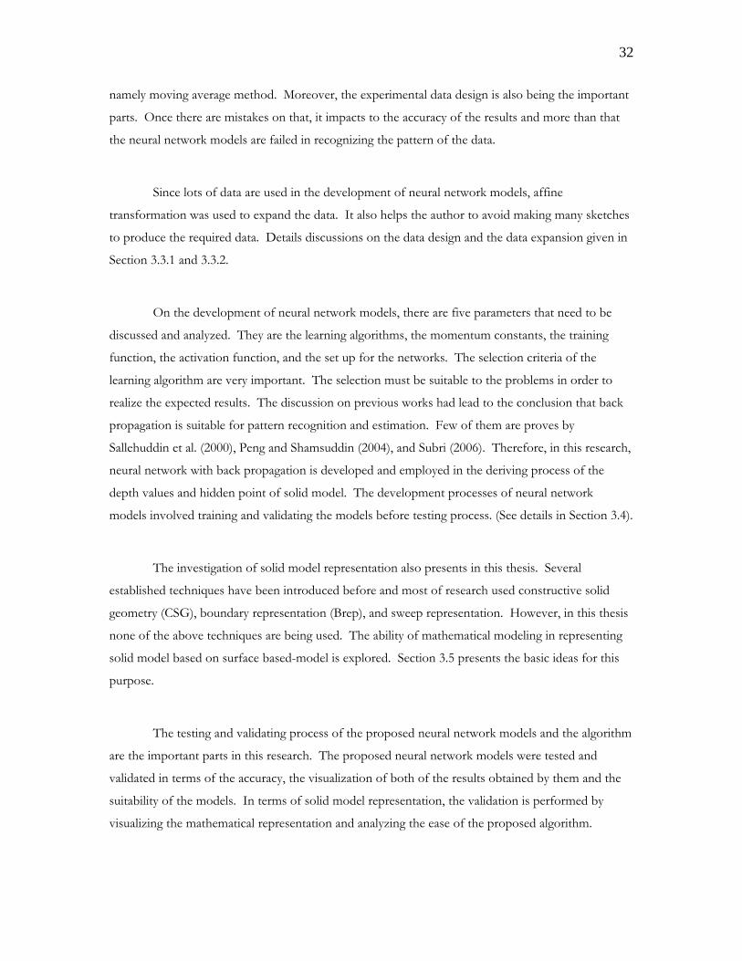
32
namely moving average method. Moreover, the experimental data design is also being the important
parts. Once there are mistakes on that, it impacts to the accuracy of the results and more than that
the neural network models are failed in recognizing the pattern of the data.
Since lots of data are used in the development of neural network models, affine
transformation was used to expand the data. It also helps the author to avoid making many sketches
to produce the required data. Details discussions on the data design and the data expansion given in
Section 3.3.1 and 3.3.2.
On the development of neural network models, there are five parameters that need to be
discussed and analyzed. They are the learning algorithms, the momentum constants, the training
function, the activation function, and the set up for the networks. The selection criteria of the
learning algorithm are very important. The selection must be suitable to the problems in order to
realize the expected results. The discussion on previous works had lead to the conclusion that back
propagation is suitable for pattern recognition and estimation. Few of them are proves by
Sallehuddin et al. (2000), Peng and Shamsuddin (2004), and Subri (2006). Therefore, in this research,
neural network with back propagation is developed and employed in the deriving process of the
depth values and hidden point of solid model. The development processes of neural network
models involved training and validating the models before testing process. (See details in Section 3.4).
The investigation of solid model representation also presents in this thesis. Several
established techniques have been introduced before and most of research used constructive solid
geometry (CSG), boundary representation (Brep), and sweep representation. However, in this thesis
none of the above techniques are being used. The ability of mathematical modeling in representing
solid model based on surface based-model is explored. Section 3.5 presents the basic ideas for this
purpose.
The testing and validating process of the proposed neural network models and the algorithm
are the important parts in this research. The proposed neural network models were tested and
validated in terms of the accuracy, the visualization of both of the results obtained by them and the
suitability of the models. In terms of solid model representation, the validation is performed by
visualizing the mathematical representation and analyzing the ease of the proposed algorithm.
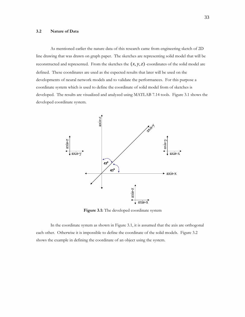
33
3.2 Nature of Data
As mentioned earlier the nature data of this research came from engineering sketch of 2D
line drawing that was drawn on graph paper. The sketches are representing solid model that will be
reconstructed and represented. From the sketches the ( , , )x y z -coordinates of the solid model are
defined. These coordinates are used as the expected results that later will be used on the
developments of neural network models and to validate the performances. For this purpose a
coordinate system which is used to define the coordinate of solid model from of sketches is
developed. The results are visualized and analyzed using MATLAB 7.14 tools. Figure 3.1 shows the
developed coordinate system.
Figure 3.1: The developed coordinate system
In the coordinate system as shown in Figure 3.1, it is assumed that the axis are orthogonal
each other. Otherwise it is impossible to define the coordinate of the solid models. Figure 3.2
shows the example in defining the coordinate of an object using the system.
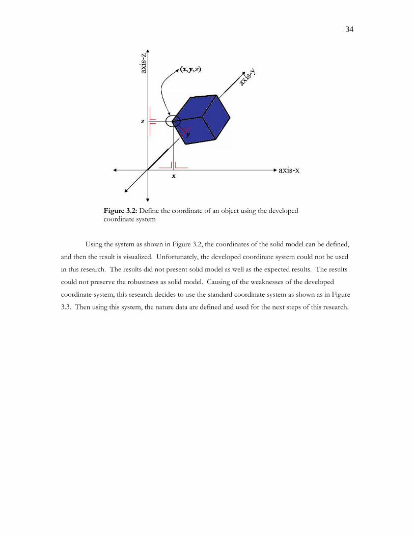
34
Figure 3.2: Define the coordinate of an object using the developed coordinate system
Using the system as shown in Figure 3.2, the coordinates of the solid model can be defined,
and then the result is visualized. Unfortunately, the developed coordinate system could not be used
in this research. The results did not present solid model as well as the expected results. The results
could not preserve the robustness as solid model. Causing of the weaknesses of the developed
coordinate system, this research decides to use the standard coordinate system as shown as in Figure
3.3. Then using this system, the nature data are defined and used for the next steps of this research.
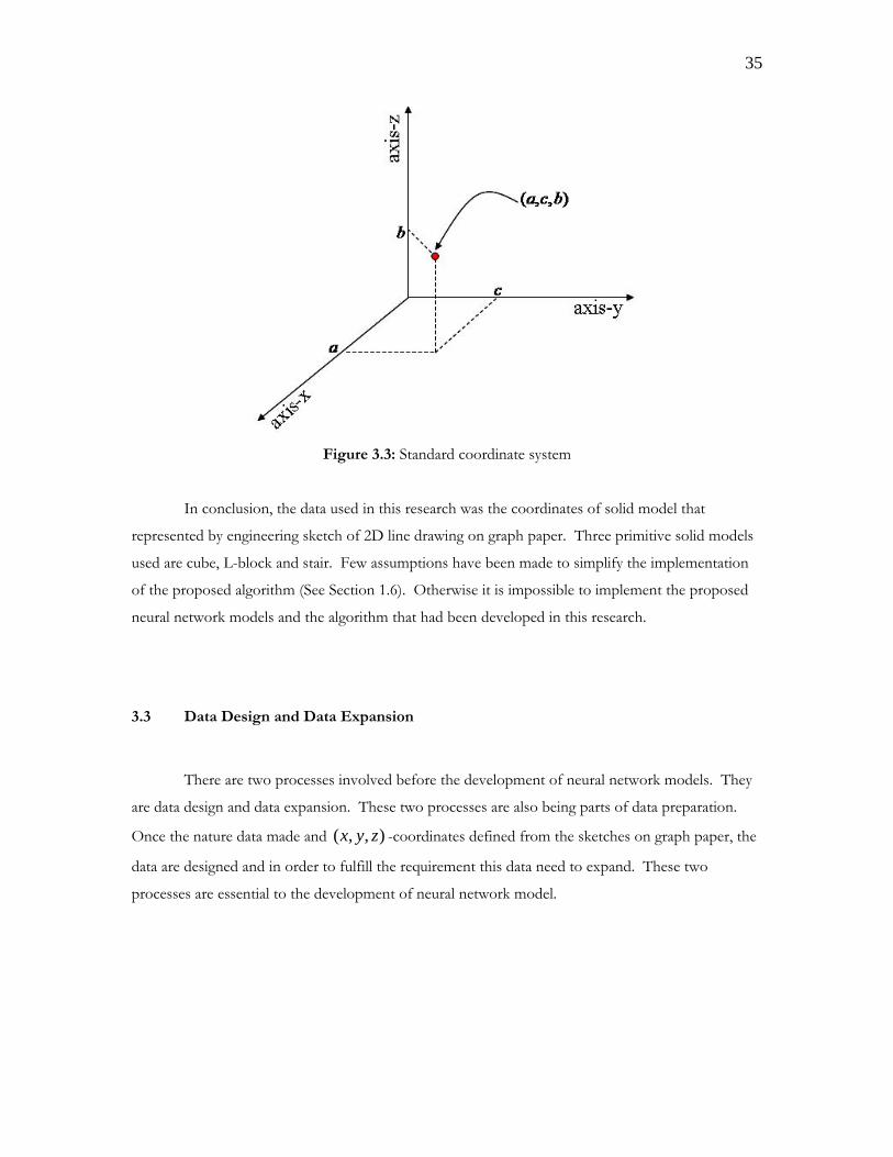
35
Figure 3.3: Standard coordinate system
In conclusion, the data used in this research was the coordinates of solid model that
represented by engineering sketch of 2D line drawing on graph paper. Three primitive solid models
used are cube, L-block and stair. Few assumptions have been made to simplify the implementation
of the proposed algorithm (See Section 1.6). Otherwise it is impossible to implement the proposed
neural network models and the algorithm that had been developed in this research.
3.3 Data Design and Data Expansion
There are two processes involved before the development of neural network models. They
are data design and data expansion. These two processes are also being parts of data preparation.
Once the nature data made and ( , , )x y z -coordinates defined from the sketches on graph paper, the
data are designed and in order to fulfill the requirement this data need to expand. These two
processes are essential to the development of neural network model.
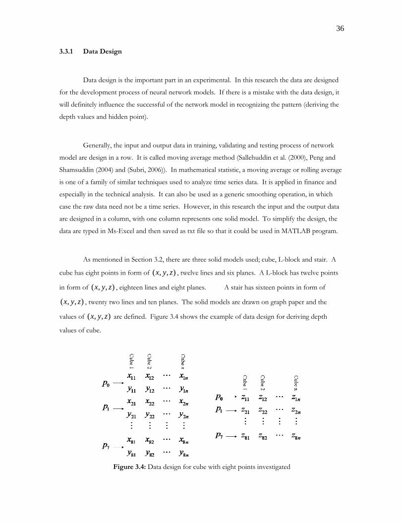
36
3.3.1 Data Design
Data design is the important part in an experimental. In this research the data are designed
for the development process of neural network models. If there is a mistake with the data design, it
will definitely influence the successful of the network model in recognizing the pattern (deriving the
depth values and hidden point).
Generally, the input and output data in training, validating and testing process of network
model are design in a row. It is called moving average method (Sallehuddin et al. (2000), Peng and
Shamsuddin (2004) and (Subri, 2006)). In mathematical statistic, a moving average or rolling average
is one of a family of similar techniques used to analyze time series data. It is applied in finance and
especially in the technical analysis. It can also be used as a generic smoothing operation, in which
case the raw data need not be a time series. However, in this research the input and the output data
are designed in a column, with one column represents one solid model. To simplify the design, the
data are typed in Ms-Excel and then saved as txt file so that it could be used in MATLAB program.
As mentioned in Section 3.2, there are three solid models used; cube, L-block and stair. A
cube has eight points in form of ( , , )x y z , twelve lines and six planes. A L-block has twelve points
in form of ( , , )x y z , eighteen lines and eight planes. A stair has sixteen points in form of
( , , )x y z , twenty two lines and ten planes. The solid models are drawn on graph paper and the
values of ( , , )x y z are defined. Figure 3.4 shows the example of data design for deriving depth
values of cube.
Figure 3.4: Data design for cube with eight points investigated
37
For each solid model the ( , )x y -value is used as the input data and the z -value is used as
the output data. It means that there are sixteen inputs and eight outputs data for each cube, twenty
four inputs and twelve outputs data for each L-block, and thirty two inputs and sixteen outputs data
for each stair.
3.3.2 Data Expansion
Many data is needed in the development process of neural network models. Thus a lot of
sketches must be drawn on graph paper and then extract the coordinates. However, to simplify and
skip the process, there is only one sketch is drawn for each solid model, and then it is transformed to
generate the other required data.
Generally in mathematics, a transformation or mapping, in elementary terms is any of a
variety of different functions from geometry, such as translation, reflection and rotation. A
translation, or translation operator, is an affine transformation of Euclidean space which moves every
point by a fixed distance in the same direction. It can also be interpreted as the addition of a
constant vector to every point, or as shifting the origin of the coordinate system. In other words, if
v is a fixed vector, then the translation vT is defined as
( )vT p p v= + . (3.1)
with p is the index of the translation.
A reflection is a map that transforms an object into its mirror image. For example, a
reflection of the small English letter p in respect to a vertical line would look like q. In order to
reflect a planar figure, one need the ‘mirror’ to be a line (‘axis of reflection’), while for reflections in
the three-dimensional space one would use a plane for a mirror. Reflection sometimes is considered
as a special case of inversion with infinite radius of the reference circle.
A rotation is a movement of an object in a circular motion. Mathematically, a rotation is,
unlike a translation, a rigid body movement which keeps a point fixed. This definition applies to
rotations within both two and three dimensions (in a plane and in space, respectively. A rotation in
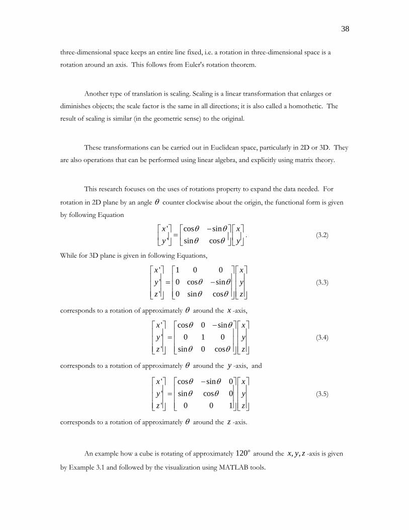
38
three-dimensional space keeps an entire line fixed, i.e. a rotation in three-dimensional space is a
rotation around an axis. This follows from Euler's rotation theorem.
Another type of translation is scaling. Scaling is a linear transformation that enlarges or
diminishes objects; the scale factor is the same in all directions; it is also called a homothetic. The
result of scaling is similar (in the geometric sense) to the original.
These transformations can be carried out in Euclidean space, particularly in 2D or 3D. They
are also operations that can be performed using linear algebra, and explicitly using matrix theory.
This research focuses on the uses of rotations property to expand the data needed. For
rotation in 2D plane by an angle θ counter clockwise about the origin, the functional form is given
by following Equation
' cos sin' sin cos
x xy y
θ θθ θ
−⎡ ⎤ ⎡ ⎤ ⎡ ⎤=⎢ ⎥ ⎢ ⎥ ⎢ ⎥
⎣ ⎦ ⎣ ⎦ ⎣ ⎦. (3.2)
While for 3D plane is given in following Equations,
' 1 0 0' 0 cos sin' 0 sin cos
x xy yz z
θ θθ θ
⎡ ⎤ ⎡ ⎤ ⎡ ⎤⎢ ⎥ ⎢ ⎥ ⎢ ⎥= −⎢ ⎥ ⎢ ⎥ ⎢ ⎥⎢ ⎥ ⎢ ⎥ ⎢ ⎥⎣ ⎦ ⎣ ⎦ ⎣ ⎦
(3.3)
corresponds to a rotation of approximately θ around the x -axis,
' cos 0 sin' 0 1 0' sin 0 cos
x xy yz z
θ θ
θ θ
−⎡ ⎤ ⎡ ⎤ ⎡ ⎤⎢ ⎥ ⎢ ⎥ ⎢ ⎥=⎢ ⎥ ⎢ ⎥ ⎢ ⎥⎢ ⎥ ⎢ ⎥ ⎢ ⎥⎣ ⎦ ⎣ ⎦ ⎣ ⎦
(3.4)
corresponds to a rotation of approximately θ around the y -axis, and
' cos sin 0' sin cos 0' 0 0 1
x xy yz z
θ θθ θ
−⎡ ⎤ ⎡ ⎤ ⎡ ⎤⎢ ⎥ ⎢ ⎥ ⎢ ⎥=⎢ ⎥ ⎢ ⎥ ⎢ ⎥⎢ ⎥ ⎢ ⎥ ⎢ ⎥⎣ ⎦ ⎣ ⎦ ⎣ ⎦
(3.5)
corresponds to a rotation of approximately θ around the z -axis.
An example how a cube is rotating of approximately 120o around the , ,x y z -axis is given
by Example 3.1 and followed by the visualization using MATLAB tools.
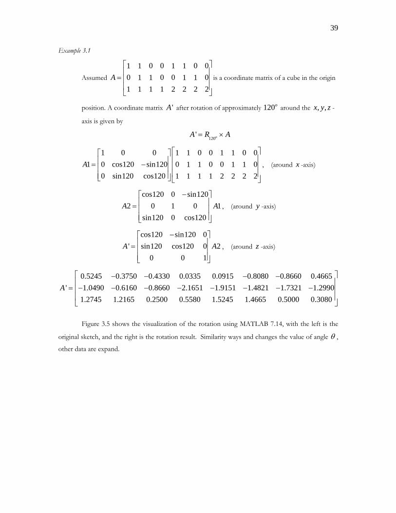
39
Example 3.1
Assumed
0 0 0 01 1 1 10 0 0 01 1 1 11 1 1 1 2 2 2 2
A⎡ ⎤⎢ ⎥
= ⎢ ⎥⎢ ⎥⎣ ⎦
is a coordinate matrix of a cube in the origin
position. A coordinate matrix 'A after rotation of approximately 120o around the , ,x y z -
axis is given by
120' oA R A= ×
1 0 0 0 0 0 01 1 1 11 0 cos120 sin120 0 0 0 01 1 1 1
0 sin120 cos120 1 1 1 1 2 2 2 2A
⎡ ⎤⎡ ⎤⎢ ⎥⎢ ⎥= − ⎢ ⎥⎢ ⎥⎢ ⎥⎢ ⎥⎣ ⎦ ⎣ ⎦
, (around x -axis)
cos120 0 sin1202 0 1 0 1
sin120 0 cos120A A
−⎡ ⎤⎢ ⎥= ⎢ ⎥⎢ ⎥⎣ ⎦
, (around y -axis)
cos120 sin120 0' sin120 cos120 0 2
0 0 1A A
−⎡ ⎤⎢ ⎥= ⎢ ⎥⎢ ⎥⎣ ⎦
, (around z -axis)
0.5245 0.3750 0.4330 0.0335 0.0915 0.8080 0.8660 0.4665' 1.0490 0.6160 0.8660 2.1651 1.9151 1.4821 1.7321 1.2990
1.2745 1.2165 0.2500 0.5580 1.5245 1.4665 0.5000 0.3080A
⎡ ⎤− − − −⎢ ⎥
= − − − − − − − −⎢ ⎥⎢ ⎥⎣ ⎦
Figure 3.5 shows the visualization of the rotation using MATLAB 7.14, with the left is the
original sketch, and the right is the rotation result. Similarity ways and changes the value of angle θ ,
other data are expand.
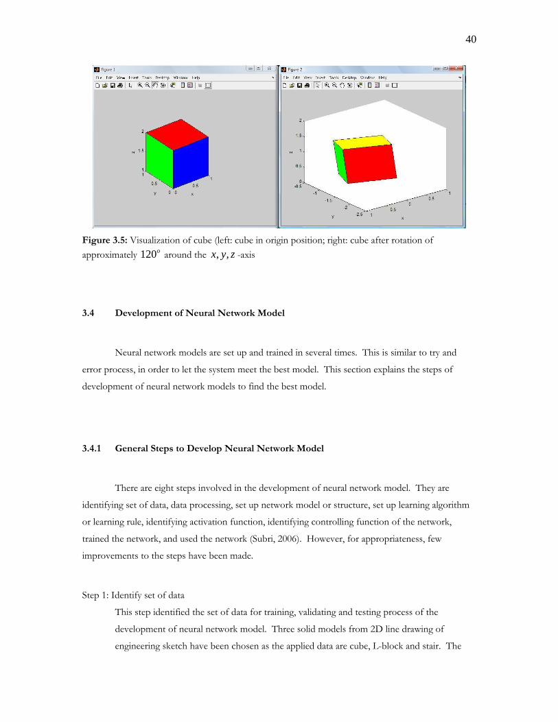
40
Figure 3.5: Visualization of cube (left: cube in origin position; right: cube after rotation of approximately 120o around the , ,x y z -axis
3.4 Development of Neural Network Model
Neural network models are set up and trained in several times. This is similar to try and
error process, in order to let the system meet the best model. This section explains the steps of
development of neural network models to find the best model.
3.4.1 General Steps to Develop Neural Network Model
There are eight steps involved in the development of neural network model. They are
identifying set of data, data processing, set up network model or structure, set up learning algorithm
or learning rule, identifying activation function, identifying controlling function of the network,
trained the network, and used the network (Subri, 2006). However, for appropriateness, few
improvements to the steps have been made.
Step 1: Identify set of data
This step identified the set of data for training, validating and testing process of the
development of neural network model. Three solid models from 2D line drawing of
engineering sketch have been chosen as the applied data are cube, L-block and stair. The
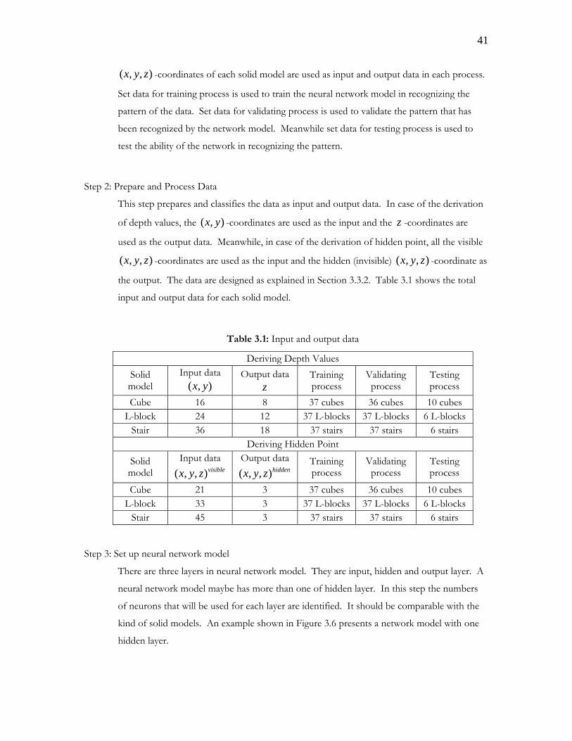
41
( , , )x y z -coordinates of each solid model are used as input and output data in each process.
Set data for training process is used to train the neural network model in recognizing the
pattern of the data. Set data for validating process is used to validate the pattern that has
been recognized by the network model. Meanwhile set data for testing process is used to
test the ability of the network in recognizing the pattern.
Step 2: Prepare and Process Data
This step prepares and classifies the data as input and output data. In case of the derivation
of depth values, the ( , )x y -coordinates are used as the input and the z -coordinates are
used as the output data. Meanwhile, in case of the derivation of hidden point, all the visible
( , , )x y z -coordinates are used as the input and the hidden (invisible) ( , , )x y z -coordinate as
the output. The data are designed as explained in Section 3.3.2. Table 3.1 shows the total
input and output data for each solid model.
Table 3.1: Input and output data
Deriving Depth Values Solid model
Input data ( , )x y
Output data z
Training process
Validating process
Testing process
Cube 16 8 37 cubes 36 cubes 10 cubes L-block 24 12 37 L-blocks 37 L-blocks 6 L-blocks
Stair 36 18 37 stairs 37 stairs 6 stairs Deriving Hidden Point
Solid model
Input data ( , , )visiblex y z
Output data ( , , )hiddenx y z
Training process
Validating process
Testing process
Cube 21 3 37 cubes 36 cubes 10 cubes L-block 33 3 37 L-blocks 37 L-blocks 6 L-blocks
Stair 45 3 37 stairs 37 stairs 6 stairs
Step 3: Set up neural network model
There are three layers in neural network model. They are input, hidden and output layer. A
neural network model maybe has more than one of hidden layer. In this step the numbers
of neurons that will be used for each layer are identified. It should be comparable with the
kind of solid models. An example shown in Figure 3.6 presents a network model with one
hidden layer.
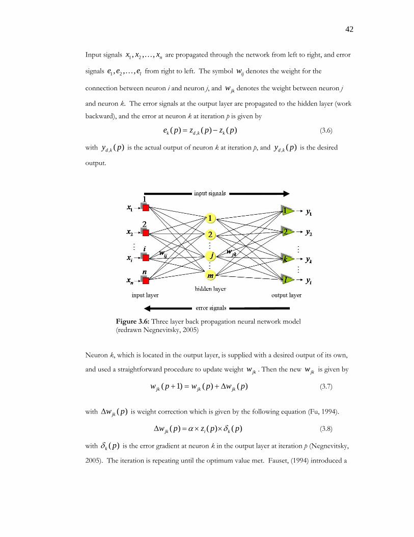
42
Input signals 1 2, , , nx x xK are propagated through the network from left to right, and error
signals 1 2, , , le e eK from right to left. The symbol ijw denotes the weight for the
connection between neuron i and neuron j, and jkw denotes the weight between neuron j
and neuron k. The error signals at the output layer are propagated to the hidden layer (work
backward), and the error at neuron k at iteration p is given by
,( ) ( ) ( )k d k ke p z p z p= − (3.6)
with , ( )d ky p is the actual output of neuron k at iteration p, and , ( )d ky p is the desired
output.
Figure 3.6: Three layer back propagation neural network model (redrawn Negnevitsky, 2005)
Neuron k, which is located in the output layer, is supplied with a desired output of its own,
and used a straightforward procedure to update weight jkw . Then the new jkw is given by
( 1) ( ) ( )jk jk jkw p w p w p+ = + ∆ (3.7)
with ( )jkw p∆ is weight correction which is given by the following equation (Fu, 1994).
( ) ( ) ( )jk i kw p z p pα δ∆ = × × (3.8)
with ( )k pδ is the error gradient at neuron k in the output layer at iteration p (Negnevitsky,
2005). The iteration is repeating until the optimum value met. Fauset, (1994) introduced a
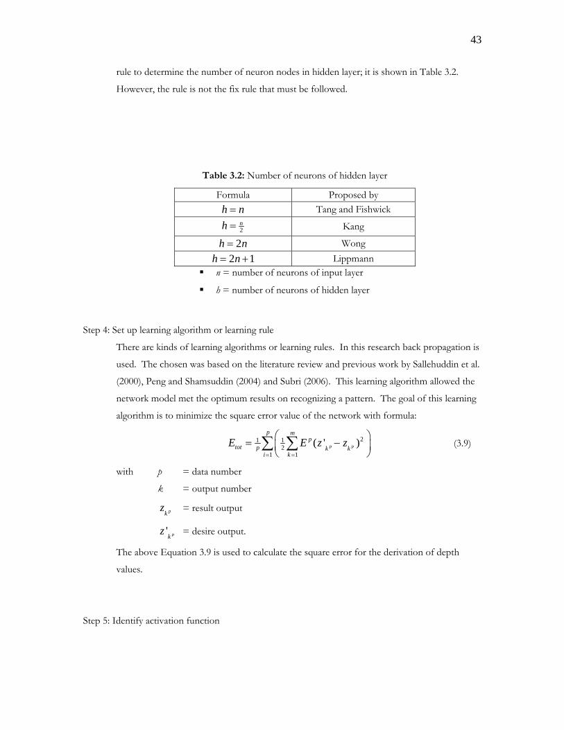
43
rule to determine the number of neuron nodes in hidden layer; it is shown in Table 3.2.
However, the rule is not the fix rule that must be followed.
Table 3.2: Number of neurons of hidden layer
Formula Proposed by h n= Tang and Fishwick
2nh = Kang
2h n= Wong 2 1h n= + Lippmann
n = number of neurons of input layer
h = number of neurons of hidden layer
Step 4: Set up learning algorithm or learning rule
There are kinds of learning algorithms or learning rules. In this research back propagation is
used. The chosen was based on the literature review and previous work by Sallehuddin et al.
(2000), Peng and Shamsuddin (2004) and Subri (2006). This learning algorithm allowed the
network model met the optimum results on recognizing a pattern. The goal of this learning
algorithm is to minimize the square error value of the network with formula:
21 12
1 1
( ' )p p
p mp
tot p k ki k
E E z z= =
⎛ ⎞= −⎜ ⎟⎝ ⎠
∑ ∑ (3.9)
with p = data number
k = output number
pkz = result output
' pkz = desire output.
The above Equation 3.9 is used to calculate the square error for the derivation of depth
values.
Step 5: Identify activation function
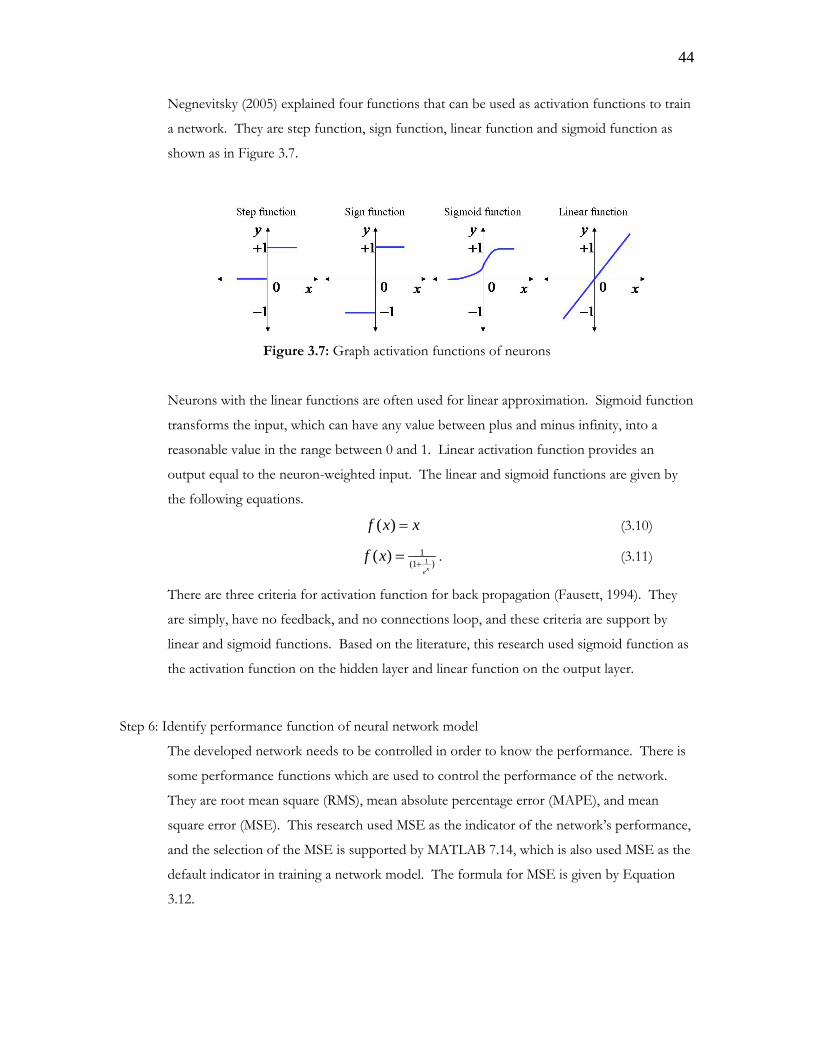
44
Negnevitsky (2005) explained four functions that can be used as activation functions to train
a network. They are step function, sign function, linear function and sigmoid function as
shown as in Figure 3.7.
Figure 3.7: Graph activation functions of neurons
Neurons with the linear functions are often used for linear approximation. Sigmoid function
transforms the input, which can have any value between plus and minus infinity, into a
reasonable value in the range between 0 and 1. Linear activation function provides an
output equal to the neuron-weighted input. The linear and sigmoid functions are given by
the following equations.
( )f x x= (3.10)
11
(1 )( )
xe
f x+
= . (3.11)
There are three criteria for activation function for back propagation (Fausett, 1994). They
are simply, have no feedback, and no connections loop, and these criteria are support by
linear and sigmoid functions. Based on the literature, this research used sigmoid function as
the activation function on the hidden layer and linear function on the output layer.
Step 6: Identify performance function of neural network model
The developed network needs to be controlled in order to know the performance. There is
some performance functions which are used to control the performance of the network.
They are root mean square (RMS), mean absolute percentage error (MAPE), and mean
square error (MSE). This research used MSE as the indicator of the network’s performance,
and the selection of the MSE is supported by MATLAB 7.14, which is also used MSE as the
default indicator in training a network model. The formula for MSE is given by Equation
3.12.
45
2( )n
ii
e
nMSE∑
= (3.12)
with ie is the ith error.
Step 7: Train the neural network model
When the network trained, the process is stopped if the MSE value meets the goal value.
Otherwise, the network failed to recognize the pattern and the result are produced with a big
error value. In this research, the goal for MSE value was determined as 0.01.
Step 8: Test the neural network model
Once the neural network models trained and validated with the goal met, then the models
ready for testing purpose.
3.4.2 Back Propagation Algorithm
Back propagation has been applied as the learning algorithm of the development of neural
network models. In this section the back propagation algorithm of neural network models for
deriving depth values is given. This algorithm contains of four steps which is made based on
Negnevitsky (2005) and few improvements for the appropriateness. The steps are:
Step 1: Initialization
Set all the weights and threshold levels of the network inside a small range ( )2,42.4 ,i iF F− + ,
with Fi is the total number of neuron i in the network (Haykin, 1999). In this research, the
weights are set to the MATLAB give the random value. The weight initialization is set on a
neuron-by-neuron basis.
Step 2: Activation
Activate the back propagation neural network by applying inputs
1 1 2 2( ), ( ), ( ), ( ), , ( ), ( )n nx p y p x p y p x p y pK and desired outputs
,1 ,2 ,( ), ( ), , ( )d d d nz p z p z pK
Calculate the actual outputs of the neurons in the hidden layer:
46
1 1
( ) ( ) ( ) ( ) ( )n n
j i ij j i ij ji i
z p sigmoid x p w p y p w pθ θ= =
⎡ ⎤= × − ∪ × −⎢ ⎥⎣ ⎦∑ ∑ , (3.13)
with n is the number of inputs of neuron j in the hidden layer.
Calculate the actual outputs of the neurons in the output layer:
1 1( ) ( ) ( ) ( ) ( )
m m
k jk jk k jk jk kj j
z p sigmoid x p w p y p w pθ θ= =
⎡ ⎤= × − ∪ × −⎢ ⎥
⎣ ⎦∑ ∑ , (3.14)
with m is the number of inputs of the neurons k in the output layer.
Step 3: Weight training
Update the weights in the back-propagation network propagating backwards the errors
associated with output neurons.
• Calculate the error gradient for the neurons in the output layer:
[ ]( ) ( ) 1 ( ) ( )k k k kp z p z p e pδ = × − × (3.15)
,( ) ( ) ( )k d k ke p z p z p= − (3.16)
Calculate the weight corrections:
( ) ( ) ( )jk i kw p z p pα δ∆ = × × (3.17)
Update the weights at the output neurons in the hidden layer:
( 1) ( ) ( )jk jk jkw p w p w p+ = + ∆ (3.18)
• Calculate the error gradient for the neurons in the hidden layer
1( ) ( ) 1 ( ) ( ) ( )
l
j i j k jkk
p z p z p p w pδ δ=
⎡ ⎤= × − × ×⎣ ⎦ ∑ (3.19)
Calculate the weight corrections:
( ) ( ) ( ) ( ) ( )jk i j i jw p x p p y p pα δ α δ∆ = × × ∪ × × (3.20)
Update the weights at the hidden neurons:
( 1) ( ) ( )ij ij ijw p w p w p+ = + ∆ (3.21)
Step 4: Iteration
Increase iteration p by one, go back to Step 2 and repeat the process until the selected error
criterion is satisfied.
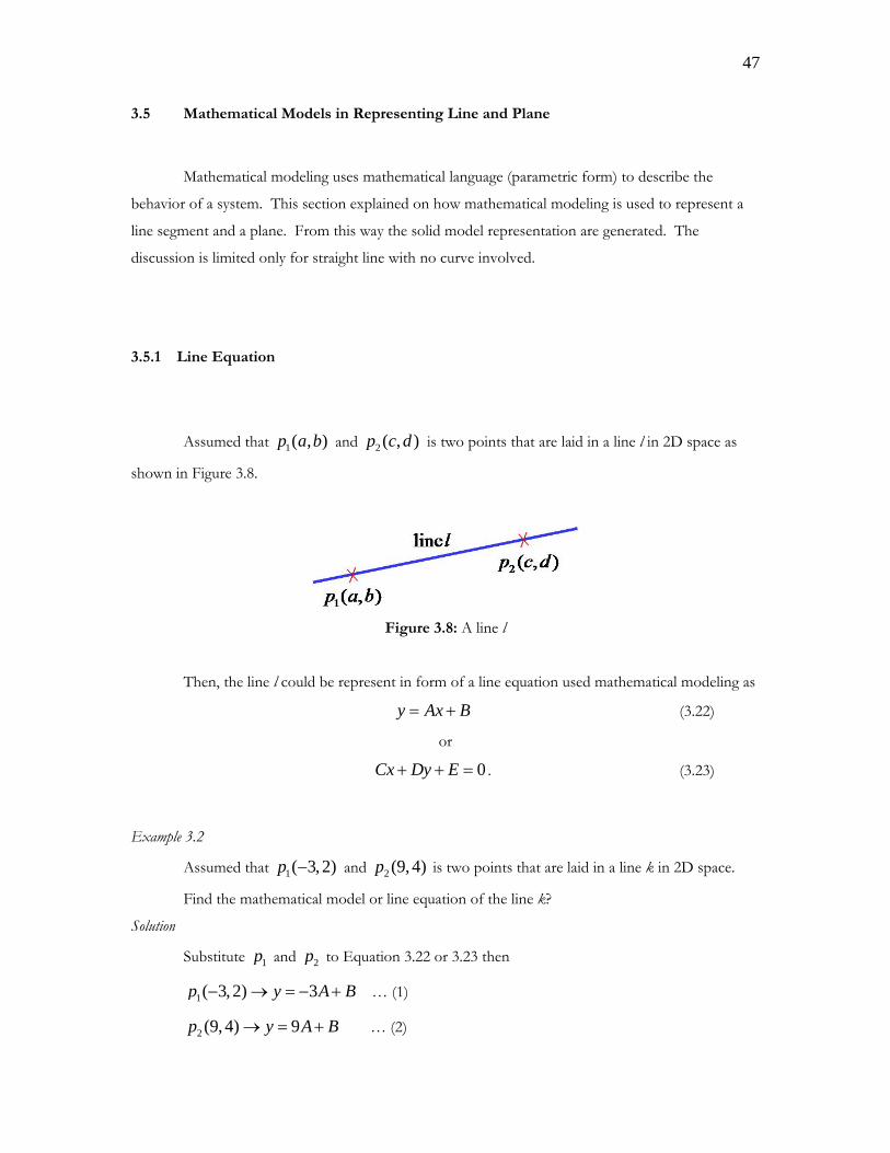
47
3.5 Mathematical Models in Representing Line and Plane
Mathematical modeling uses mathematical language (parametric form) to describe the
behavior of a system. This section explained on how mathematical modeling is used to represent a
line segment and a plane. From this way the solid model representation are generated. The
discussion is limited only for straight line with no curve involved.
3.5.1 Line Equation
Assumed that 1( , )p a b and 2 ( , )p c d is two points that are laid in a line l in 2D space as
shown in Figure 3.8.
Figure 3.8: A line l
Then, the line l could be represent in form of a line equation used mathematical modeling as
y Ax B= + (3.22)
or
0Cx Dy E+ + = . (3.23)
Example 3.2
Assumed that 1( 3, 2)p − and 2 (9, 4)p is two points that are laid in a line k in 2D space.
Find the mathematical model or line equation of the line k?
Solution
Substitute 1p and 2p to Equation 3.22 or 3.23 then
1( 3, 2) 3p y A B− → = − + … (1)
2 (9, 4) 9p y A B→ = + … (2)
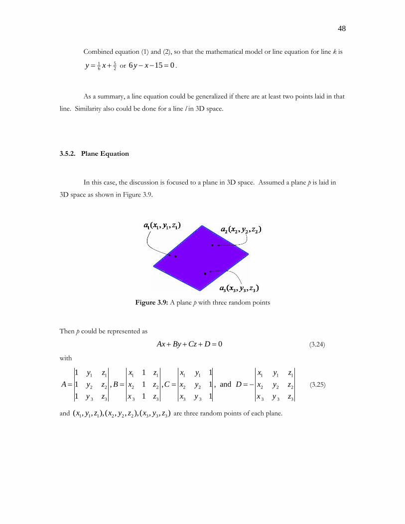
48
Combined equation (1) and (2), so that the mathematical model or line equation for line k is 51
6 2y x= + or 6 15 0y x− − = .
As a summary, a line equation could be generalized if there are at least two points laid in that
line. Similarity also could be done for a line l in 3D space.
3.5.2. Plane Equation
In this case, the discussion is focused to a plane in 3D space. Assumed a plane p is laid in
3D space as shown in Figure 3.9.
Figure 3.9: A plane p with three random points
Then p could be represented as
0Ax By Cz D+ + + = (3.24)
with
1 1 1 1 1 1 1 1 1
2 2 2 2 2 2 2 2 2
3 3 3 3 3 3 3 3 3
1 1 11 , 1 , 1 , and1 1 1
y z x z x y x y zA y z B x z C x y D x y z
y z x z x y x y z= = = = − (3.25)
and 1 1 1 2 2 2 3 3 3( , , ),( , , ),( , , )x y z x y z x y z are three random points of each plane.
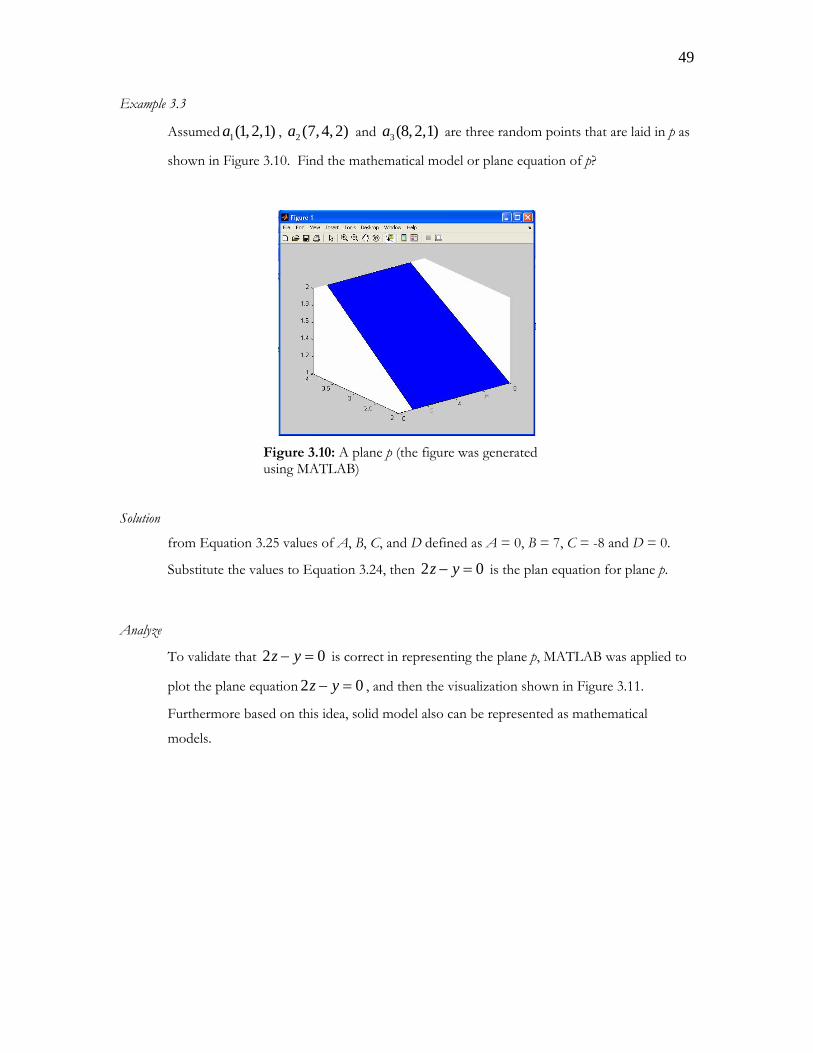
49
Example 3.3
Assumed 1(1, 2,1)a , 2 (7,4, 2)a and 3 (8, 2,1)a are three random points that are laid in p as
shown in Figure 3.10. Find the mathematical model or plane equation of p?
Figure 3.10: A plane p (the figure was generated using MATLAB)
Solution
from Equation 3.25 values of A, B, C, and D defined as A = 0, B = 7, C = -8 and D = 0.
Substitute the values to Equation 3.24, then 2 0z y− = is the plan equation for plane p.
Analyze
To validate that 2 0z y− = is correct in representing the plane p, MATLAB was applied to
plot the plane equation 2 0z y− = , and then the visualization shown in Figure 3.11.
Furthermore based on this idea, solid model also can be represented as mathematical
models.
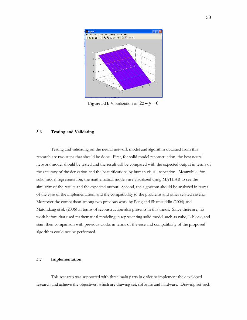
50
Figure 3.11: Visualization of 2 0z y− =
3.6 Testing and Validating
Testing and validating on the neural network model and algorithm obtained from this
research are two steps that should be done. First, for solid model reconstruction, the best neural
network model should be tested and the result will be compared with the expected output in terms of
the accuracy of the derivation and the beautifications by human visual inspection. Meanwhile, for
solid model representation, the mathematical models are visualized using MATLAB to see the
similarity of the results and the expected output. Second, the algorithm should be analyzed in terms
of the ease of the implementation, and the compatibility to the problems and other related criteria.
Moreover the comparison among two previous work by Peng and Shamsuddin (2004) and
Matondang et al. (2006) in terms of reconstruction also presents in this thesis. Since there are, no
work before that used mathematical modeling in representing solid model such as cube, L-block, and
stair, then comparison with previous works in terms of the ease and compatibility of the proposed
algorithm could not be performed.
3.7 Implementation
This research was supported with three main parts in order to implement the developed
research and achieve the objectives, which are drawing set, software and hardware. Drawing set such
51
as graph paper, pencil and ruler are used to create nature data, which are engineering sketch of 2D
line drawing of solid model. From these sketches, the ( , , )x y z are extracted and affine
transformation is employed to expand the data.
MATLAB software version 7.14 was used to implement the development of neural network
models. MATLAB 7.14 has neural network toolbox, which could be used to train network models,
validate and test the performances. Anyway this software also can be used to make a script for affine
transformation which used to expand the data from the nature, for visualization purposes, and other
calculations. Scripts in M-File mode have been used to compare the result with the expected result in
terms of the beautifications. Scripts also made to validate the mathematical models that used in
representing solid model.
A set of High End Computer with windows Vista Home Basic, specification RAM 1.5 GB
has been used to run the software program, and research works. The uses of higher RAM made the
development of neural network models run faster and will reduce the development time.
3.8 Summary
This chapter has presented the methodology of this research. The discussion was started
with the explanation to the nature data for this research. After that, the data are extracted from the
sketch on graph paper, and then expanded to fulfill the requirement data in the development process
of neural network models for solid model reconstruction. Then the discussion continued by giving
the basic idea in using mathematical models for representing solid model. Used the ideas, then a
hybrid computing algorithm in representing solid model is produced by combining the neural
network and the mathematical model. In addition, the discussion to all the components used in this
research also presented in this chapter including the testing and validating the neural network model
and the algorithm obtained.
In terms of solid model reconstruction, which used soft computing technique, the discussion
explained in details the process to the development of neural network models to achieve the best
network model for cube, L-block and stair reconstruction. The size of input and output, the
52
parameters, the learning algorithm or rule, the activation function, the network structure and the
processes involved in using MATLAB 7.14 explained in this chapter.
In terms of representation, this chapter explained the basic ideas of the uses of mathematical
models in representing solid model, with given explanations to the uses of mathematical models for
line segment and plane representation. Chapter 4 presents the data and discussion for solid model
reconstruction and representation.
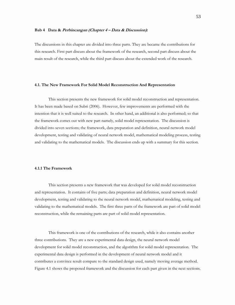
53
Bab 4 Data & Perbincangan (Chapter 4 – Data & Discussion):
The discussions in this chapter are divided into three parts. They are became the contributions for
this research. First part discuss about the framework of the research, second part discuss about the
main result of the research, while the third part discuss about the extended work of the research.
4.1. The New Framework For Solid Model Reconstruction And Representation
This section presents the new framework for solid model reconstruction and representation.
It has been made based on Subri (2006). However, few improvements are performed with the
intention that it is well suited to the research. In other hand, an additional is also performed; so that
the framework comes out with new part namely, solid model representation. The discussion is
divided into seven sections; the framework, data preparation and definition, neural network model
development, testing and validating of neural network model, mathematical modeling process, testing
and validating to the mathematical models. The discussion ends up with a summary for this section.
4.1.1 The Framework
This section presents a new framework that was developed for solid model reconstruction
and representation. It contains of five parts; data preparation and definition, neural network model
development, testing and validating to the neural network model, mathematical modeling, testing and
validating to the mathematical models. The first three parts of the framework are part of solid model
reconstruction, while the remaining parts are part of solid model representation.
This framework is one of the contributions of the research, while it also contains another
three contributions. They are a new experimental data design, the neural network model
development for solid model reconstruction, and the algorithm for solid model representation. The
experimental data design is performed in the development of neural network model and it
contributes a convince result compare to the standard design used, namely moving average method.
Figure 4.1 shows the proposed framework and the discussion for each part given in the next sections.
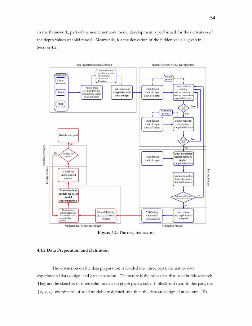
54
In the framework, part of the neural network model development is performed for the derivation of
the depth values of solid model. Meanwhile, for the derivation of the hidden value is given in
Section 4.2.
Figure 4.1: The new framework
4.1.2 Data Preparation and Definition
The discussion on the data preparation is divided into three parts; the nature data,
experimental data design, and data expansion. The nature is the prior data that used in this research.
They are the sketches of three solid models on graph paper; cube, L-block and stair. In this part, the
( , , )x y z -coordinates of solid models are defined, and then the data are designed in column. To
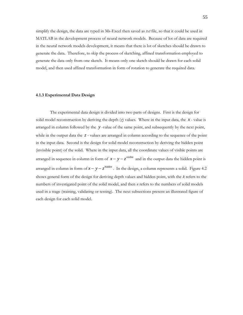
55
simplify the design, the data are typed in Ms-Excel then saved as txt file, so that it could be used in
MATLAB in the development process of neural network models. Because of lot of data are required
in the neural network models development, it means that there is lot of sketches should be drawn to
generate the data. Therefore, to skip the process of sketching, affined transformation employed to
generate the data only from one sketch. It means only one sketch should be drawn for each solid
model, and then used affined transformation in form of rotation to generate the required data.
4.1.3 Experimental Data Design
The experimental data design is divided into two parts of designs. First is the design for
solid model reconstruction by deriving the depth (z) values. Where in the input data, the x - value is
arranged in column followed by the y -value of the same point, and subsequently by the next point,
while in the output data the z - values are arranged in column according to the sequence of the point
in the input data. Second is the design for solid model reconstruction by deriving the hidden point
(invisible point) of the solid. Where in the input data, all the coordinate values of visible points are
arranged in sequence in column in form of visiblex y z− − and in the output data the hidden point is
arranged in column in form of hiddenx y z− − . In the design, a column represents a solid. Figure 4.2
shows general form of the design for deriving depth values and hidden point, with the k refers to the
numbers of investigated point of the solid model, and then n refers to the numbers of solid models
used in a stage (training, validating or testing). The next subsections present an illustrated figure of
each design for each solid model.
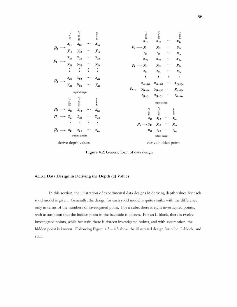
56
derive depth values derive hidden point
Figure 4.2: Generic form of data design
4.1.3.1 Data Design in Deriving the Depth (z) Values
In this section, the illustration of experimental data designs in deriving depth values for each
solid model is given. Generally, the design for each solid model is quite similar with the difference
only in terms of the numbers of investigated point. For a cube, there is eight investigated points,
with assumption that the hidden point in the backside is known. For an L-block, there is twelve
investigated points, while for stair, there is sixteen investigated points, and with assumption, the
hidden point is known. Following Figure 4.3 – 4.5 show the illustrated design for cube, L-block, and
stair.
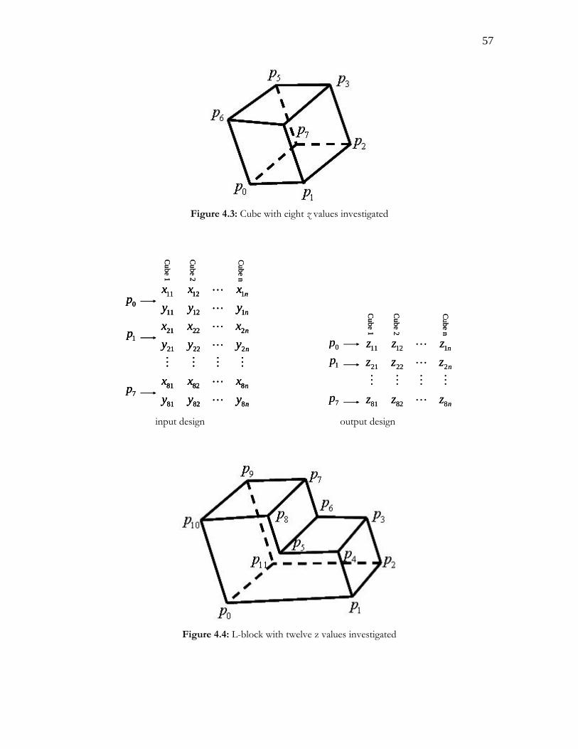
57
Figure 4.3: Cube with eight z values investigated
11 12 1
11 12 1
21 22 2
21 22 2
81 82 8
81 82 8
n
n
n
n
n
n
x x xy y yx x xy y y
x x xy y y
L
L
L
L
M M M M
L
L
0p
1p
7p
Cube 1
Cube 2
Cube n
11 12 1
11 12 1
21 22 2
21 22 2
81 82 8
81 82 8
n
n
n
n
n
n
x x xy y yx x xy y y
x x xy y y
L
L
L
L
M M M M
L
L
0p
1p
7p
11 12 1
11 12 1
21 22 2
21 22 2
81 82 8
81 82 8
n
n
n
n
n
n
x x xy y yx x xy y y
x x xy y y
L
L
L
L
M M M M
L
L
0p
1p
7p
Cube 1
Cube 2
Cube n
11 12 1
21 22 2
81 82 8
n
n
n
z z zz z z
z z z
L
L
M M M M
L
0p
1p
7p
Cube 1
Cube 2
Cube n
11 12 1
21 22 2
81 82 8
n
n
n
z z zz z z
z z z
L
L
M M M M
L
0p
1p
7p
Cube 1
Cube 2
Cube n
input design output design
Figure 4.4: L-block with twelve z values investigated
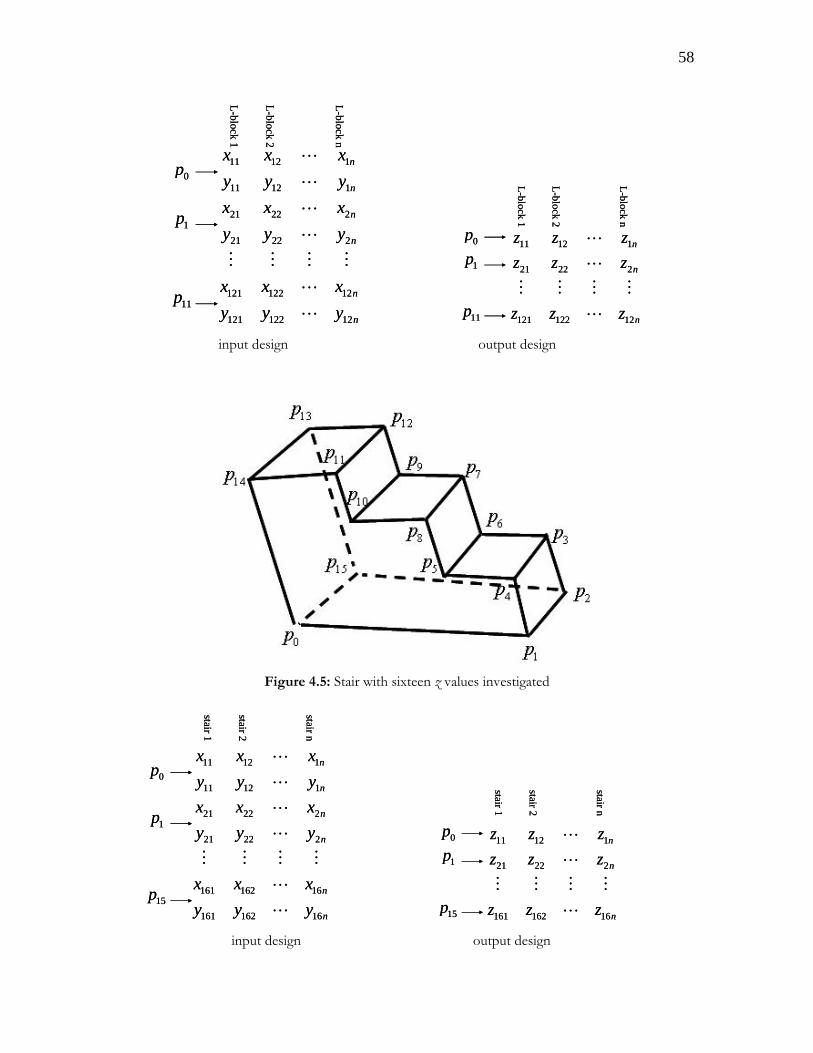
58
11 12 1
11 12 1
21 22 2
21 22 2
121 122 12
121 122 12
n
n
n
n
n
n
x x xy y yx x xy y y
x x xy y y
L
L
L
L
M M M M
L
L
0p
1p
11p
L-block 1
L-block 2
L-block n
11 12 1
11 12 1
21 22 2
21 22 2
121 122 12
121 122 12
n
n
n
n
n
n
x x xy y yx x xy y y
x x xy y y
L
L
L
L
M M M M
L
L
0p
1p
11p
L-block 1
L-block 2
L-block n
11 12 1
21 22 2
121 122 12
n
n
n
z z zz z z
z z z
L
L
M M M M
L
0p
1p
11pL-block 1
L-block 2
L-block n
11 12 1
21 22 2
121 122 12
n
n
n
z z zz z z
z z z
L
L
M M M M
L
0p
1p
11pL-block 1
L-block 2
L-block n
input design output design
Figure 4.5: Stair with sixteen z values investigated
11 12 1
11 12 1
21 22 2
21 22 2
161 162 16
161 162 16
n
n
n
n
n
n
x x xy y yx x xy y y
x x xy y y
L
L
L
L
M M M M
L
L
0p
1p
15p
stair 1
stair 2
stair n
11 12 1
11 12 1
21 22 2
21 22 2
161 162 16
161 162 16
n
n
n
n
n
n
x x xy y yx x xy y y
x x xy y y
L
L
L
L
M M M M
L
L
0p
1p
15p
stair 1
stair 2
stair n
11 12 1
21 22 2
161 162 16
n
n
n
z z zz z z
z z z
L
L
M M M M
L
0p
1p
15p
stair 1
stair 2
stair n
11 12 1
21 22 2
161 162 16
n
n
n
z z zz z z
z z z
L
L
M M M M
L
0p
1p
15p
stair 1
stair 2
stair n
input design output design
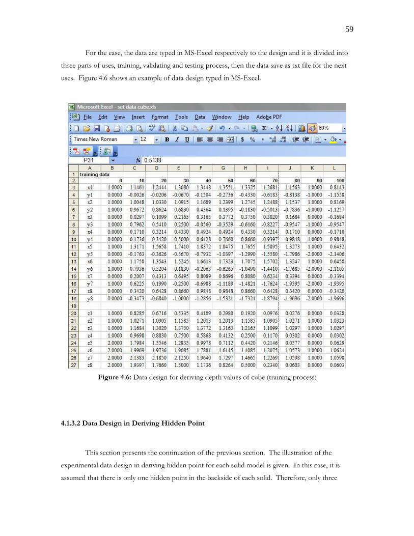
59
For the ease, the data are typed in MS-Excel respectively to the design and it is divided into
three parts of uses, training, validating and testing process, then the data save as txt file for the next
uses. Figure 4.6 shows an example of data design typed in MS-Excel.
Figure 4.6: Data design for deriving depth values of cube (training process)
4.1.3.2 Data Design in Deriving Hidden Point
This section presents the continuation of the previous section. The illustration of the
experimental data design in deriving hidden point for each solid model is given. In this case, it is
assumed that there is only one hidden point in the backside of each solid. Therefore, only three
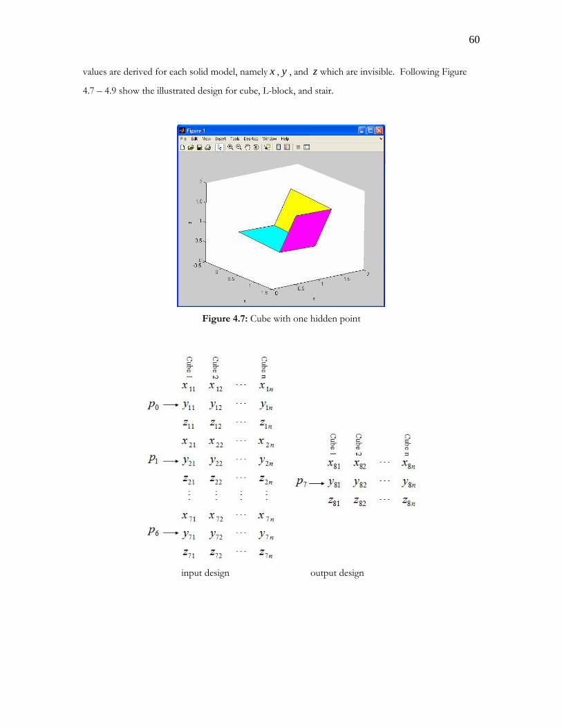
60
values are derived for each solid model, namely x , y , and z which are invisible. Following Figure
4.7 – 4.9 show the illustrated design for cube, L-block, and stair.
Figure 4.7: Cube with one hidden point
input design output design
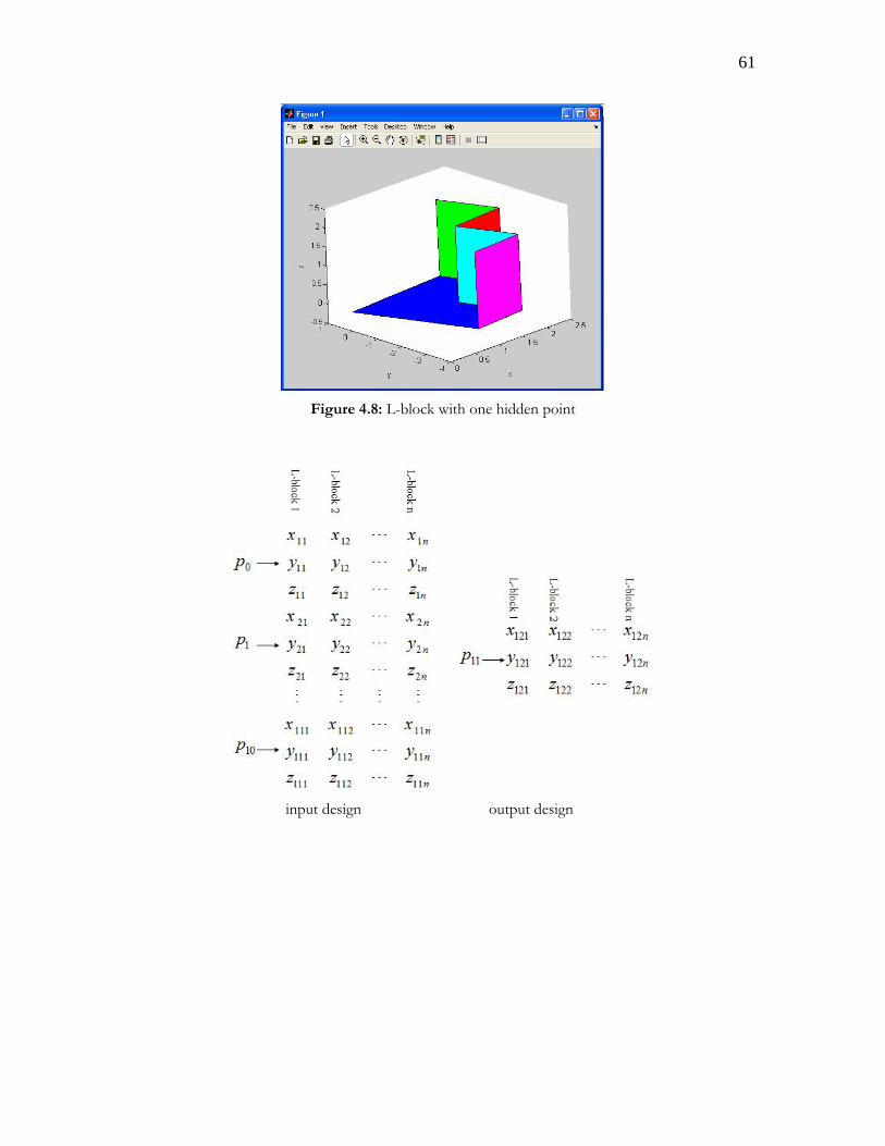
61
Figure 4.8: L-block with one hidden point
input design output design
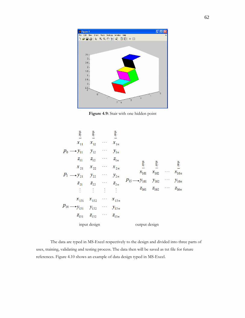
62
Figure 4.9: Stair with one hidden point
input design output design
The data are typed in MS-Excel respectively to the design and divided into three parts of
uses, training, validating and testing process. The data then will be saved as txt file for future
references. Figure 4.10 shows an example of data design typed in MS-Excel.
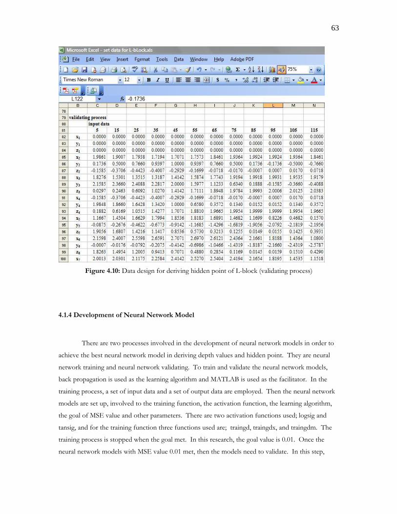
63
Figure 4.10: Data design for deriving hidden point of L-block (validating process)
4.1.4 Development of Neural Network Model
There are two processes involved in the development of neural network models in order to
achieve the best neural network model in deriving depth values and hidden point. They are neural
network training and neural network validating. To train and validate the neural network models,
back propagation is used as the learning algorithm and MATLAB is used as the facilitator. In the
training process, a set of input data and a set of output data are employed. Then the neural network
models are set up, involved to the training function, the activation function, the learning algorithm,
the goal of MSE value and other parameters. There are two activation functions used; logsig and
tansig, and for the training function three functions used are; traingd, traingdx, and traingdm. The
training process is stopped when the goal met. In this research, the goal value is 0.01. Once the
neural network models with MSE value 0.01 met, then the models need to validate. In this step,
64
another set of input and output data are employed. Then the same process as like as in training
process did, and the process stop if the goal met. Details discussions of the neural network models
development for both two types of reconstruction; by deriving depth values and deriving hidden
point are given in Section 4.2.
4.1.5 Testing and Validating of Neural Network Model
Once the neural network models with MSE value equals or less then 0.01 are met, then these
models are tested. For that purpose, a set of input data are employed to the neural network models,
and the testing process to obtain the results is performed. In this process a neural network model is
tested in several times and the neural network model with the smallest MSE value is defined as the
best neural network model. In this research, the author defines MSE values interval between 0.0030
– 0.0060 as smallest value. In other words, if the MSE value of the testing process lay in the interval,
then the neural network model is defined as the best model.
Next step, after the testing process completed, then the result obtained necessitate to be
validated to perceive the accuracy of the derivation and to observe the beautifications by human
visual inspection. The validation process also used MATLAB program.
4.1.6 Mathematical Modeling Process
In this part, the reconstructed solid models are represented based on surface based model
used mathematical representation. The representation used the coordinates of the reconstructed
solid then combined with mathematical models to generate the mathematical representation of the
reconstructed solid. The mathematical modeling process contains of three stages. First is defining
( , , )x y z -coordinates of the reconstructed solid. Second is generating the plane equations of the
reconstructed solid. Third is generating the mathematical representation of the reconstructed solid.
For generating the plane equations of the solid, two rules could be performed; determinant rules and
Gauss-Jordan method. In conjunction with the solid models that used in this research, there are six
plane equations for a cube, eight plane equations for L-block and ten plane equations for a stair.
65
4.1.7 Testing and Validating the Mathematical Models
To test the ability of mathematical modeling in representing solid model, the ( , , )x y z -
coordinates of the solid should be known. In this research the ( , , )x y z -coordinates are originated
from the reconstructed solid model and Gauss-Jordan method is used to generate the mathematical
representation (mathematical model).
After the coordinates of the reconstructed solid model defined, then the mathematical
representation is generated, subsequently the representation (the model) is visualized to perceive the
correctness and compared to the original solid model. Details discussion of the mathematical
modeling process is given in Section 4.3 and for overall process MATLAB also used.
4.1.8 Summary
This section has presented a complete framework for both solid model reconstruction and
representation of 2D line drawing. It contains of five parts; data preparation and definition, neural
network model development, testing and validation for the developed neural network models,
mathematical modeling process of the reconstructed solid models, and then testing and validating for
mathematical representation of the reconstructed solids.
A brief discussion to the contributions of the research is also presented in this section. They
are a new experimental data design for the development process of neural network models, the
proposed neural network models for solid model reconstruction from single view image of 2D line
drawing, and new algorithm for solid model representation from given 2D line drawing which is
called as hybrid computing algorithm in representing solid model. Detail explanations about the
development of neural network models for solid model reconstruction and the developed algorithm
for solid model representation are given in the next section.
66
4.2. The Neural Network Model Development
This section explains in details about the development process of neural network models,
which is used for solid model reconstruction from given single view image of 2D line drawing. The
discussions are divided into four sections; an introduction and motivation for the work, neural
network model development for deriving depth values, neural network model development for
deriving hidden point, and a summary. The experimental result on how the developed neural
network models are implemented also given in this section.
4.2.1 Introduction and Motivation
There are several established techniques for solid model reconstruction that have been
introduced before. They are related to mathematical modeling and manipulation on geometrical
analysis. However, since the era of soft computing draw closers, some researches did not deal with
exact techniques anymore. The uses of soft computing techniques have become a new tremendous
solution for solid model reconstruction problems. Some previous works on that are presented in
Section 2.6.2. Unfortunately, many reports and papers described the techniques for solid model
reconstruction, which are related to mathematical modeling, geometrical analysis, and soft computing
techniques, are not suitable for solid model reconstruction from single view image of 2D line
drawing. Therefore, this thesis presents a new technique based on the uses of soft computing
technique, that can be used to reconstruct solid model from given single view image of 2D line
drawing. The process can be categorized into two parts; reconstruction by deriving depth values and
reconstruction by deriving hidden point of solid models. To accomplish the objectives, neural
network models are developed.
4.2.2 Neural Network Model Development for Deriving Depth Values
In Section 2.5, a brief discussion of neural network model has been given, and followed by
Section 3.4, which explained the general steps in developing neural network model for pattern
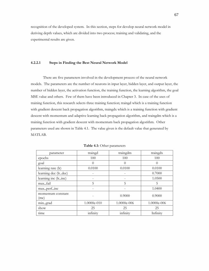
67
recognition of the developed system. In this section, steps for develop neural network model in
deriving depth values, which are divided into two process; training and validating, and the
experimental results are given.
4.2.2.1 Steps in Finding the Best Neural Network Model
There are five parameters involved in the development process of the neural network
models. The parameters are the number of neurons in input layer, hidden layer, and output layer, the
number of hidden layer, the activation function, the training function, the learning algorithm, the goal
MSE value and others. Few of them have been introduced in Chapter 3. In case of the uses of
training function, this research selects three training function; traingd which is a training function
with gradient descent back propagation algorithm, traingdx which is a training function with gradient
descent with momentum and adaptive learning back propagation algorithm, and traingdm which is a
training function with gradient descent with momentum back propagation algorithm. Other
parameters used are shown in Table 4.1. The value given is the default value that generated by
MATLAB.
Table 4.1: Other parameters
parameter traingd traingdm traingdx epochs 100 100 100 goal 0 0 0 learning rate (lr) 0.0100 0.0100 0.0100 learning dec (lr_dec) - - 0.7000 learning inc (lr_inc) - - 1.0500 max_fail 5 5 5 max_perf_inc - - 1.0400 momentum constant (mc) - 0.9000 0.9000
min_grad 1.0000e-010 1.0000e-006 1.0000e-006 show 25 25 25 time infinity infinity Infinity
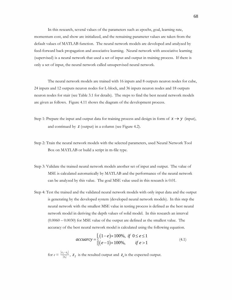
68
In this research, several values of the parameters such as epochs, goal, learning rate,
momentum cost, and show are initialized, and the remaining parameter values are taken from the
default values of MATLAB function. The neural network models are developed and analyzed by
feed-forward back propagation and associative learning. Neural network with associative learning
(supervised) is a neural network that used a set of input and output in training process. If there is
only a set of input, the neural network called unsupervised neural network.
The neural network models are trained with 16 inputs and 8 outputs neuron nodes for cube,
24 inputs and 12 outputs neuron nodes for L-block, and 36 inputs neuron nodes and 18 outputs
neuron nodes for stair (see Table 3.1 for details). The steps to find the best neural network models
are given as follows. Figure 4.11 shows the diagram of the development process.
Step 1: Prepare the input and output data for training process and design in form of x y→ (input),
and continued by z (output) in a column (see Figure 4.2).
Step 2: Train the neural network models with the selected parameters, used Neural Network Tool
Box on MATLAB or build a script in m-file type.
Step 3: Validate the trained neural network models another set of input and output. The value of
MSE is calculated automatically by MATLAB and the performance of the neural network
can be analyzed by this value. The goal MSE value used in this research is 0.01.
Step 4: Test the trained and the validated neural network models with only input data and the output
is generating by the developed system (developed neural network models). In this step the
neural network with the smallest MSE value in testing process is defined as the best neural
network model in deriving the depth values of solid model. In this research an interval
(0.0060 – 0.0030) for MSE value of the output are defined as the smallest value. The
accuracy of the best neural network model is calculated using the following equation.
( )( )1 100%, 0 1
1 100%, 1e if e
accuarcye if e− × ≤ ≤⎧⎪= ⎨ − × >⎪⎩
(4.1)
for e = f e
e
z zz−
, fz is the resulted output and ez is the expected output.
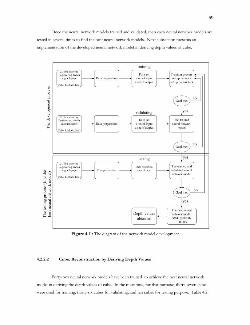
69
Once the neural network models trained and validated, then each neural network models are
tested in several times to find the best neural network models. Next subsection presents an
implementation of the developed neural network model in deriving depth values of cube.
Figure 4.11: The diagram of the network model development
4.2.2.2 Cube: Reconstruction by Deriving Depth Values
Forty-two neural network models have been trained to achieve the best neural network
model in deriving the depth values of cube. In the meantime, for that purpose, thirty-seven cubes
were used for training, thirty-six cubes for validating, and ten cubes for testing purpose. Table 4.2
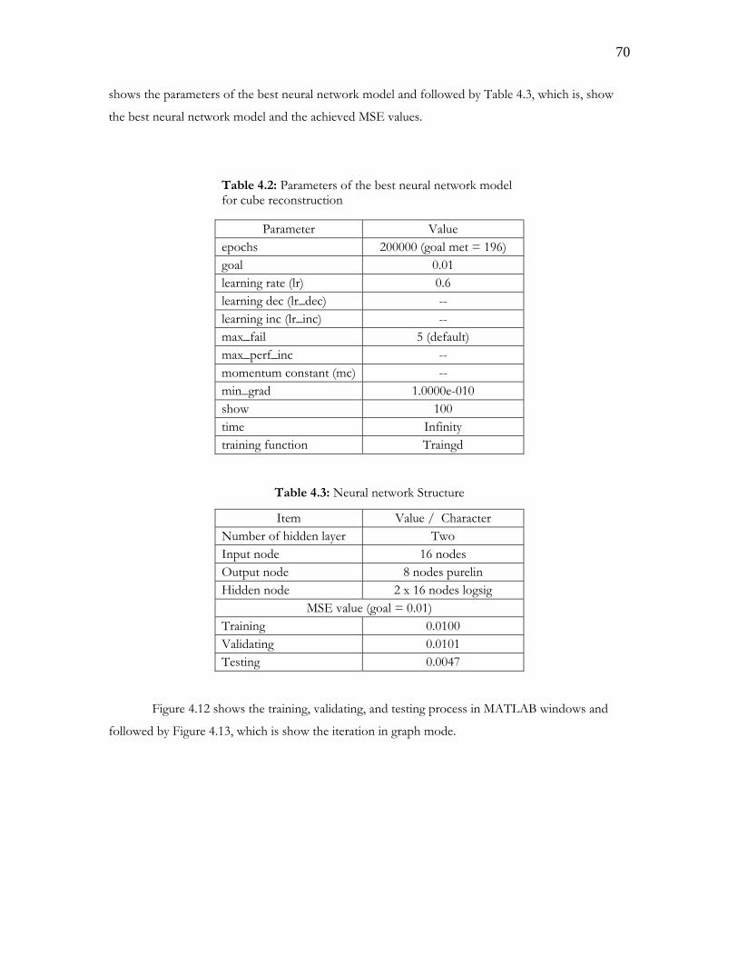
70
shows the parameters of the best neural network model and followed by Table 4.3, which is, show
the best neural network model and the achieved MSE values.
Table 4.2: Parameters of the best neural network model for cube reconstruction
Parameter Value epochs 200000 (goal met = 196) goal 0.01 learning rate (lr) 0.6 learning dec (lr_dec) -- learning inc (lr_inc) -- max_fail 5 (default) max_perf_inc -- momentum constant (mc) -- min_grad 1.0000e-010 show 100 time Infinity training function Traingd
Table 4.3: Neural network Structure
Item Value / Character Number of hidden layer Two Input node 16 nodes Output node 8 nodes purelin Hidden node 2 x 16 nodes logsig
MSE value (goal = 0.01) Training 0.0100 Validating 0.0101 Testing 0.0047
Figure 4.12 shows the training, validating, and testing process in MATLAB windows and
followed by Figure 4.13, which is show the iteration in graph mode.
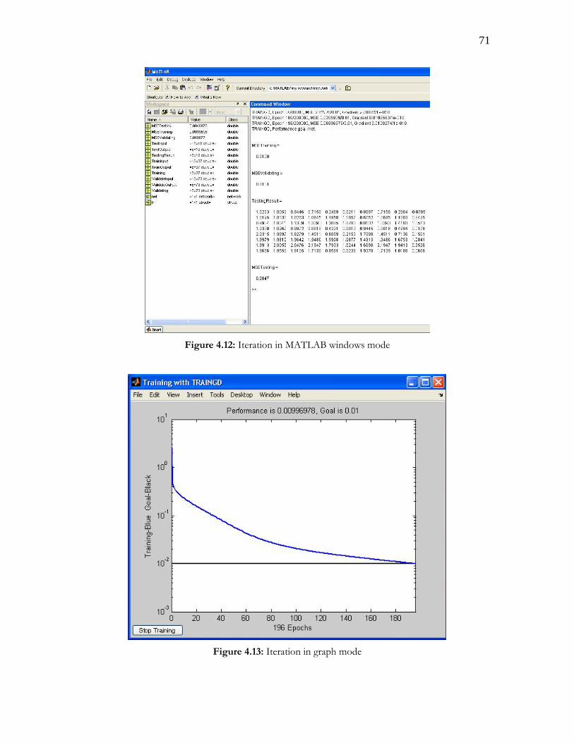
71
Figure 4.12: Iteration in MATLAB windows mode
Figure 4.13: Iteration in graph mode
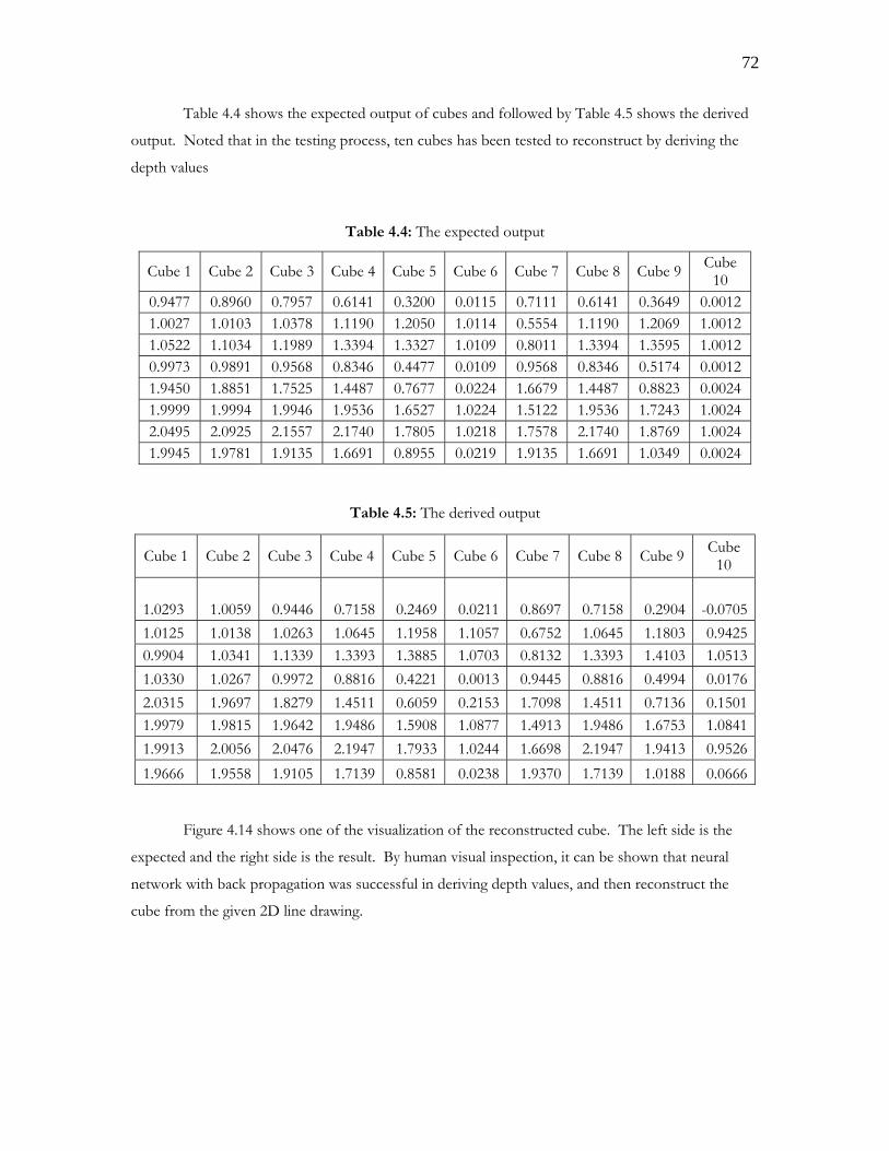
72
Table 4.4 shows the expected output of cubes and followed by Table 4.5 shows the derived
output. Noted that in the testing process, ten cubes has been tested to reconstruct by deriving the
depth values
Table 4.4: The expected output
Cube 1 Cube 2 Cube 3 Cube 4 Cube 5 Cube 6 Cube 7 Cube 8 Cube 9 Cube 10
0.9477 0.8960 0.7957 0.6141 0.3200 0.0115 0.7111 0.6141 0.3649 0.00121.0027 1.0103 1.0378 1.1190 1.2050 1.0114 0.5554 1.1190 1.2069 1.00121.0522 1.1034 1.1989 1.3394 1.3327 1.0109 0.8011 1.3394 1.3595 1.00120.9973 0.9891 0.9568 0.8346 0.4477 0.0109 0.9568 0.8346 0.5174 0.00121.9450 1.8851 1.7525 1.4487 0.7677 0.0224 1.6679 1.4487 0.8823 0.00241.9999 1.9994 1.9946 1.9536 1.6527 1.0224 1.5122 1.9536 1.7243 1.00242.0495 2.0925 2.1557 2.1740 1.7805 1.0218 1.7578 2.1740 1.8769 1.00241.9945 1.9781 1.9135 1.6691 0.8955 0.0219 1.9135 1.6691 1.0349 0.0024
Table 4.5: The derived output
Cube 1 Cube 2 Cube 3 Cube 4 Cube 5 Cube 6 Cube 7 Cube 8 Cube 9 Cube 10
1.0293 1.0059 0.9446 0.7158 0.2469 0.0211 0.8697 0.7158 0.2904 -0.07051.0125 1.0138 1.0263 1.0645 1.1958 1.1057 0.6752 1.0645 1.1803 0.94250.9904 1.0341 1.1339 1.3393 1.3885 1.0703 0.8132 1.3393 1.4103 1.05131.0330 1.0267 0.9972 0.8816 0.4221 0.0013 0.9445 0.8816 0.4994 0.01762.0315 1.9697 1.8279 1.4511 0.6059 0.2153 1.7098 1.4511 0.7136 0.15011.9979 1.9815 1.9642 1.9486 1.5908 1.0877 1.4913 1.9486 1.6753 1.08411.9913 2.0056 2.0476 2.1947 1.7933 1.0244 1.6698 2.1947 1.9413 0.95261.9666 1.9558 1.9105 1.7139 0.8581 0.0238 1.9370 1.7139 1.0188 0.0666
Figure 4.14 shows one of the visualization of the reconstructed cube. The left side is the
expected and the right side is the result. By human visual inspection, it can be shown that neural
network with back propagation was successful in deriving depth values, and then reconstruct the
cube from the given 2D line drawing.
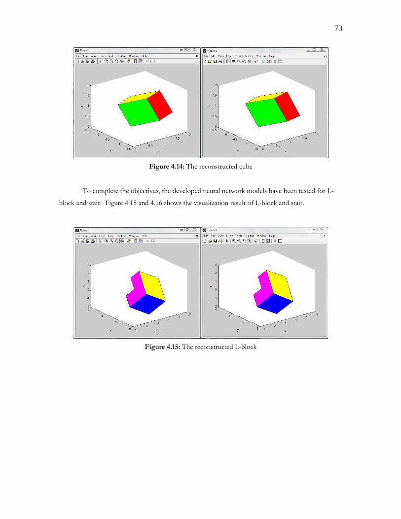
73
Figure 4.14: The reconstructed cube
To complete the objectives, the developed neural network models have been tested for L-
block and stair. Figure 4.15 and 4.16 shows the visualization result of L-block and stair.
Figure 4.15: The reconstructed L-block
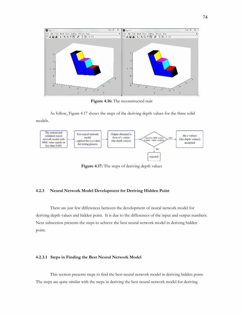
74
Figure 4.16: The reconstructed stair
As follow, Figure 4.17 shows the steps of the deriving depth values for the three solid
models.
Figure 4.17: The steps of deriving depth values
4.2.3 Neural Network Model Development for Deriving Hidden Point
There are just few differences between the development of neural network model for
deriving depth values and hidden point. It is due to the differences of the input and output numbers.
Next subsection presents the steps to achieve the best neural network model in deriving hidden
point.
4.2.3.1 Steps in Finding the Best Neural Network Model
This section presents steps to find the best neural network model in deriving hidden point.
The steps are quite similar with the steps in deriving the best neural network model for deriving
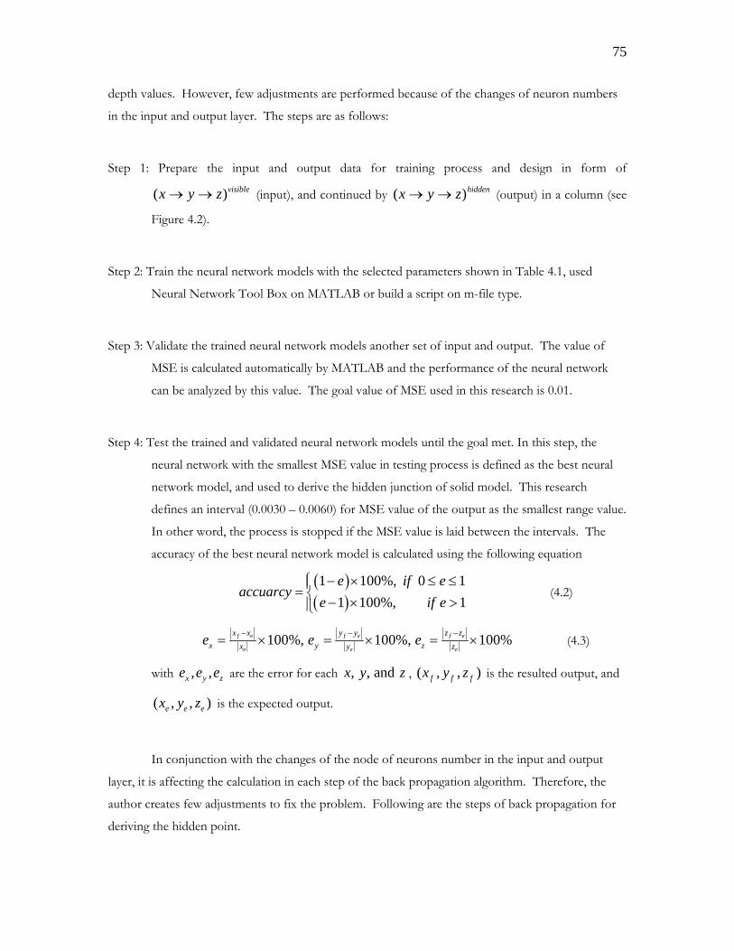
75
depth values. However, few adjustments are performed because of the changes of neuron numbers
in the input and output layer. The steps are as follows:
Step 1: Prepare the input and output data for training process and design in form of
( )visiblex y z→ → (input), and continued by ( )hiddenx y z→ → (output) in a column (see
Figure 4.2).
Step 2: Train the neural network models with the selected parameters shown in Table 4.1, used
Neural Network Tool Box on MATLAB or build a script on m-file type.
Step 3: Validate the trained neural network models another set of input and output. The value of
MSE is calculated automatically by MATLAB and the performance of the neural network
can be analyzed by this value. The goal value of MSE used in this research is 0.01.
Step 4: Test the trained and validated neural network models until the goal met. In this step, the
neural network with the smallest MSE value in testing process is defined as the best neural
network model, and used to derive the hidden junction of solid model. This research
defines an interval (0.0030 – 0.0060) for MSE value of the output as the smallest range value.
In other word, the process is stopped if the MSE value is laid between the intervals. The
accuracy of the best neural network model is calculated using the following equation
( )( )1 100%, 0 1
1 100%, 1e if e
accuarcye if e− × ≤ ≤⎧⎪= ⎨ − × >⎪⎩
(4.2)
100%, 100%, 100%f e f e f e
e e e
x x y y z zx y zx y ze e e− − −= × = × = × (4.3)
with , ,x y ze e e are the error for each , , andx y z , ( , , )f f fx y z is the resulted output, and
( , , )e e ex y z is the expected output.
In conjunction with the changes of the node of neurons number in the input and output
layer, it is affecting the calculation in each step of the back propagation algorithm. Therefore, the
author creates few adjustments to fix the problem. Following are the steps of back propagation for
deriving the hidden point.
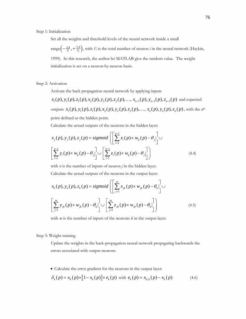
76
Step 1: Initialization
Set all the weights and threshold levels of the neural network inside a small
range ( )2,42.4 ,i iF F− + , with Fi is the total number of neuron i in the neural network (Haykin,
1999). In this research, the author let MATLAB give the random value. The weight
initialization is set on a neuron-by-neuron basis.
Step 2: Activation
Activate the back propagation neural network by applying inputs
1 1 1 2 2 2( ), ( ), ( ), ( ), ( ), ( ), ,x p y p z p x p y p z p K 1 1 1( ), ( ), ( )n n nx p y p z p− − − and expected
outputs 1 1 1 2 2 2( ), ( ), ( ), ( ), ( ), ( ), ,x p y p z p x p y p z p K ( ), ( ), ( )n n nx p y p z p , with the nth
point defined as the hidden point.
Calculate the actual outputs of the neurons in the hidden layer:
( ), ( ), ( )j j jx p y p z p sigmoid=1
1( ) ( )
n
i ij ji
x p w p θ−
=
⎛ ⎡ ⎤× − ∪⎜ ⎢ ⎥⎣ ⎦⎝
∑1
1
( ) ( )n
i ij ji
y p w p θ−
=
⎡ ⎤× − ∪⎢ ⎥⎣ ⎦∑
1
1( ) ( )
n
i ij ji
z p w p θ−
=
⎞⎡ ⎤× − ⎟⎢ ⎥⎣ ⎦ ⎠
∑ (4.4)
with n is the number of inputs of neuron j in the hidden layer.
Calculate the actual outputs of the neurons in the output layer:
( ), ( ), ( )k k kx p y p z p sigmoid=1
( ) ( )m
jk jk kj
x p w p θ=
⎛ ⎡ ⎤× − ∪⎜ ⎢ ⎥⎜ ⎣ ⎦⎝
∑
1( ) ( )
m
jk jk kj
y p w p θ=
⎡ ⎤× − ∪⎢ ⎥
⎣ ⎦∑
1( ) ( )
m
jk jk kj
z p w p θ=
⎞⎡ ⎤× − ⎟⎢ ⎥ ⎟⎣ ⎦ ⎠
∑ (4.5)
with m is the number of inputs of the neurons k in the output layer.
Step 3: Weight training
Update the weights in the back-propagation neural network propagating backwards the
errors associated with output neurons.
• Calculate the error gradient for the neurons in the output layer:
[ ]( ) ( ) 1 ( ) ( )k k k kp x p x p e pδ = × − × with ,( ) ( ) ( )k d k ke p x p x p= − (4.6)
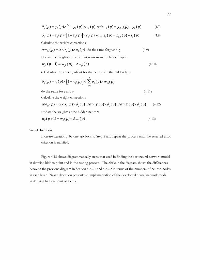
77
[ ]( ) ( ) 1 ( ) ( )k k k kp y p y p e pδ = × − × with ,( ) ( ) ( )k d k ke p y p y p= − (4.7)
[ ]( ) ( ) 1 ( ) ( )k k k kp z p z p e pδ = × − × with ,( ) ( ) ( )k d k ke p z p z p= − (4.8)
Calculate the weight corrections:
( ) ( ) ( )jk i kw p x p pα δ∆ = × × , do the same for y and z (4.9)
Update the weights at the output neurons in the hidden layer:
( 1) ( ) ( )jk jk jkw p w p w p+ = + ∆ (4.10)
• Calculate the error gradient for the neurons in the hidden layer
( ) ( ) 1 ( )j i jp x p x pδ ⎡ ⎤= × − ×⎣ ⎦1
( ) ( )l
k jkk
p w pδ=
×∑
do the same for y and z (4.11)
Calculate the weight corrections:
( ) ( ) ( )jk i jw p x p pα δ α∆ = × × ∪ × ( ) ( ) ( ) ( )i j i jy p p z p pδ α δ× ∪ × × (4.12)
Update the weights at the hidden neurons:
( 1) ( ) ( )ij ij ijw p w p w p+ = + ∆ (4.13)
Step 4: Iteration
Increase iteration p by one, go back to Step 2 and repeat the process until the selected error
criterion is satisfied.
Figure 4.18 shows diagrammatically steps that used in finding the best neural network model
in deriving hidden point and in the testing process. The circle in the diagram shows the differences
between the previous diagram in Section 4.2.2.1 and 4.2.2.2 in terms of the numbers of neuron nodes
in each layer. Next subsection presents an implementation of the developed neural network model
in deriving hidden point of a cube.
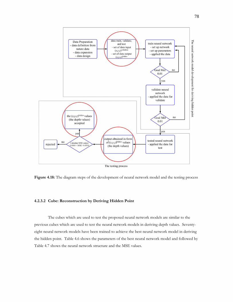
78
Figure 4.18: The diagram steps of the development of neural network model and the testing process
4.2.3.2 Cube: Reconstruction by Deriving Hidden Point
The cubes which are used to test the proposed neural network models are similar to the
previous cubes which are used to test the neural network models in deriving depth values. Seventy-
eight neural network models have been trained to achieve the best neural network model in deriving
the hidden point. Table 4.6 shows the parameters of the best neural network model and followed by
Table 4.7 shows the neural network structure and the MSE values.
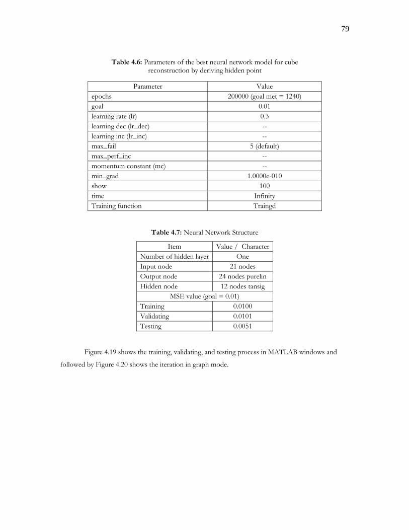
79
Table 4.6: Parameters of the best neural network model for cube
reconstruction by deriving hidden point
Parameter Value epochs 200000 (goal met = 1240) goal 0.01 learning rate (lr) 0.3 learning dec (lr_dec) -- learning inc (lr_inc) -- max_fail 5 (default) max_perf_inc -- momentum constant (mc) -- min_grad 1.0000e-010 show 100 time Infinity Training function Traingd
Table 4.7: Neural Network Structure
Item Value / CharacterNumber of hidden layer One Input node 21 nodes Output node 24 nodes purelin Hidden node 12 nodes tansig
MSE value (goal = 0.01) Training 0.0100 Validating 0.0101 Testing 0.0051
Figure 4.19 shows the training, validating, and testing process in MATLAB windows and
followed by Figure 4.20 shows the iteration in graph mode.
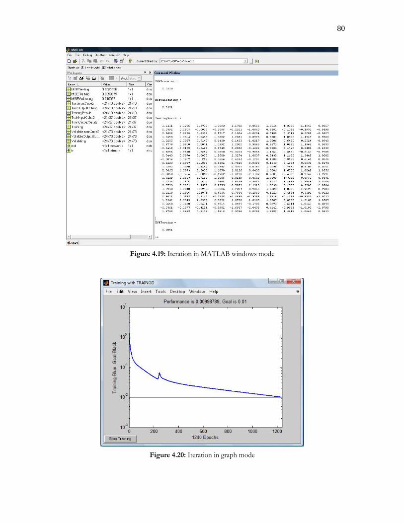
80
Figure 4.19: Iteration in MATLAB windows mode
Figure 4.20: Iteration in graph mode
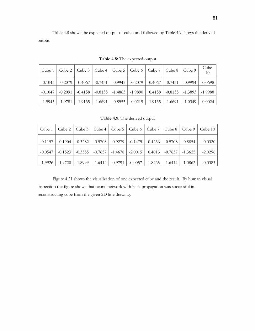
81
Table 4.8 shows the expected output of cubes and followed by Table 4.9 shows the derived
output.
Table 4.8: The expected output
Cube 1 Cube 2 Cube 3 Cube 4 Cube 5 Cube 6 Cube 7 Cube 8 Cube 9 Cube 10
0.1045 0.2079 0.4067 0.7431 0.9945 -0.2079 0.4067 0.7431 0.9994 0.0698
-0.1047 -0.2091 -0.4158 -0.8135 -1.4863 -1.9890 0.4158 -0.8135 -1.3893 -1.9988
1.9945 1.9781 1.9135 1.6691 0.8955 0.0219 1.9135 1.6691 1.0349 0.0024
Table 4.9: The derived output
Cube 1 Cube 2 Cube 3 Cube 4 Cube 5 Cube 6 Cube 7 Cube 8 Cube 9 Cube 10
0.1157 0.1904 0.3282 0.5708 0.9279 -0.1479 0.4236 0.5708 0.8854 0.0320
-0.0547 -0.1523 -0.3555 -0.7657 -1.4678 -2.0015 0.4013 -0.7657 -1.3625 -2.0296
1.9926 1.9720 1.8999 1.6414 0.9791 -0.0057 1.8465 1.6414 1.0862 -0.0383
Figure 4.21 shows the visualization of one expected cube and the result. By human visual
inspection the figure shows that neural network with back propagation was successful in
reconstructing cube from the given 2D line drawing.
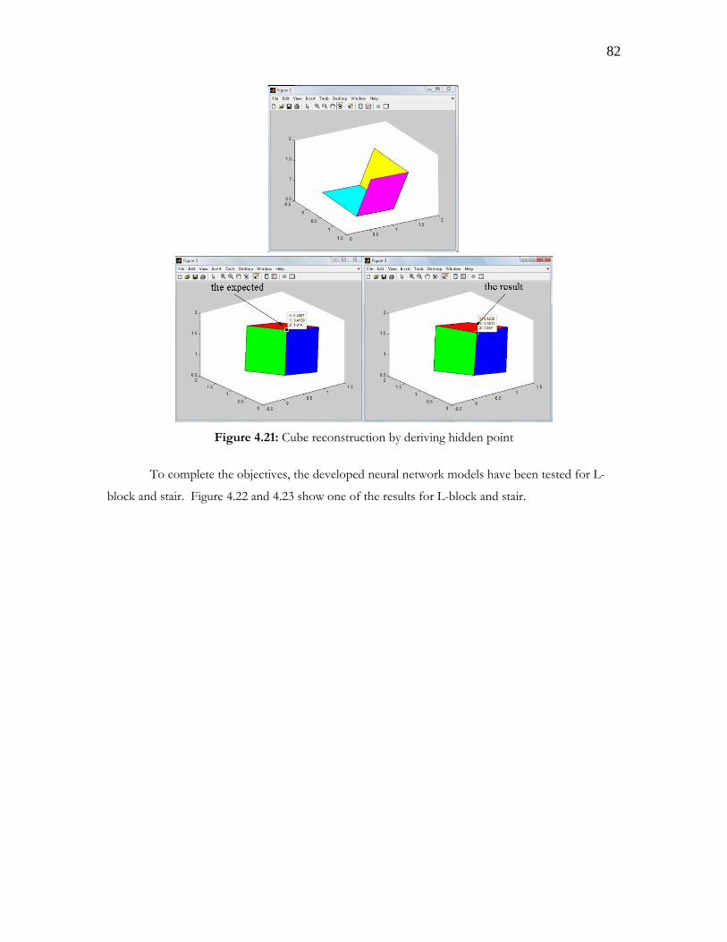
82
Figure 4.21: Cube reconstruction by deriving hidden point
To complete the objectives, the developed neural network models have been tested for L-
block and stair. Figure 4.22 and 4.23 show one of the results for L-block and stair.
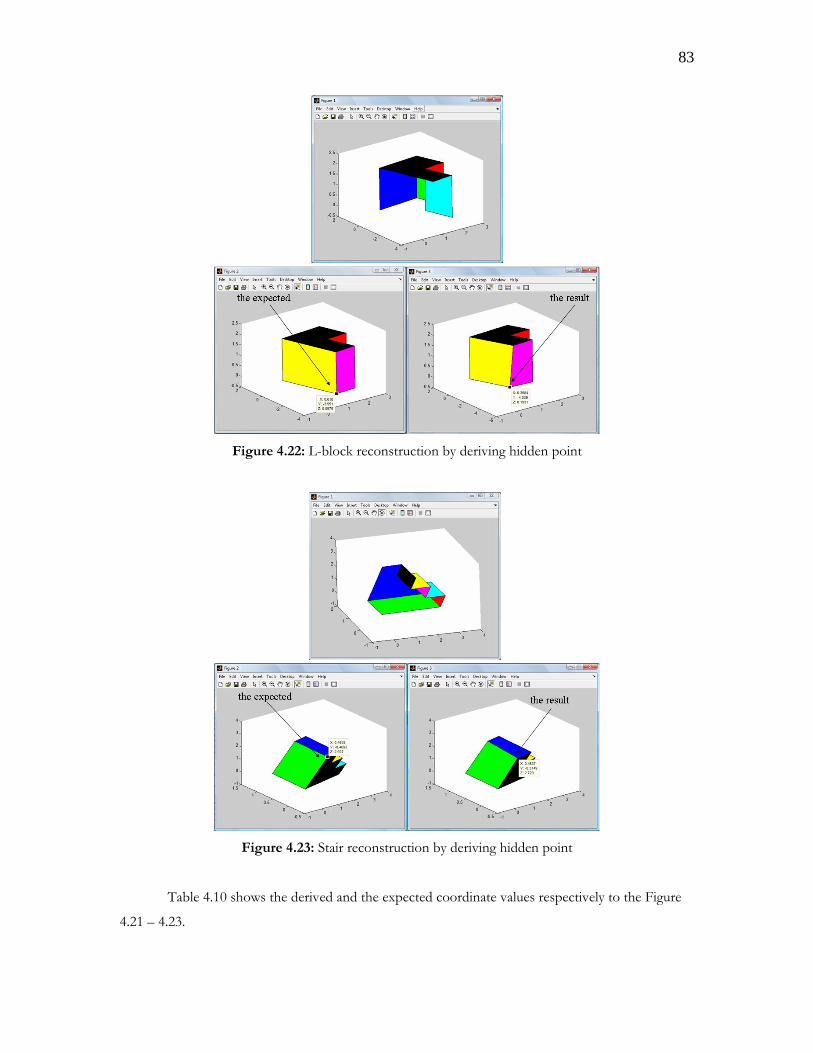
83
Figure 4.22: L-block reconstruction by deriving hidden point
Figure 4.23: Stair reconstruction by deriving hidden point
Table 4.10 shows the derived and the expected coordinate values respectively to the Figure
4.21 – 4.23.
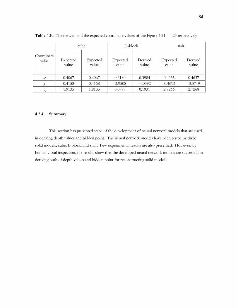
84
Table 4.10: The derived and the expected coordinate values of the Figure 4.21 – 4.23 respectively
Coordinate value
cube L-block stair
Expected value
Expected value
Expected value
Derived value
Expected value
Derived value
x 0.4067 0.4067 0.6180 0.3984 0.4635 0.4637 y 0.4158 0.4158 -3.9508 -4.0392 -0.4693 -0.3749 z 1.9135 1.9135 0.0979 0.1931 2.9266 2.7268
4.2.4 Summary
This section has presented steps of the development of neural network models that are used
in deriving depth values and hidden point. The neural network models have been tested by three
solid models; cube, L-block, and stair. Few experimental results are also presented. However, by
human visual inspection, the results show that the developed neural network models are successful in
deriving both of depth values and hidden point for reconstructing solid models.
85
4.3. Hybrid Computing Algorithm In Representing Solid Models
This section explains in details the proposed algorithm namely a hybrid-computing algorithm
in representing solid model. This work is an extended work of the development of neural network
models, and then used the output of the process as the input in mathematical modeling process to
represent solid models. In other words, the proposed algorithm contains of two parts, first is solid
model reconstruction, which employed neural network with back propagation, and second is solid
model representation, which employed mathematical modeling. Therefore, the proposed algorithm
is called a hybrid-computing algorithm in representing solid model. The discussion of this work is
divided into six sections. The first section presents the idea and motivation in using mathematical
models to represent solid model. The second section presents the hybrid-computing algorithm
followed by cube representation as one of the experimental data result. The fourth section presents
the models validation. Meanwhile the fifth section presents the discussion in representing L-plane
and stair plane. The discussion ends up with presents a summary of this section.
4.3.1 Mathematical Representation for Solid Model: Idea and Motivation
Solid modeling presents unambiguous, accuracy and completeness in 3D representation
(Lim and Mounayri, 1999). This representation is very suitable for machining process simulation
where general shape is required to be represented accurately. There are two types of solid model
representation based on mathematical models, point-set model and surface-based model.
In case of point-set model, a solid model is defined as a bounded, closed subset of the 3D
Euclidian space. The most schemes adopt are spatial decomposition modeling, and constructive
solid geometry (CSG) (Zeid, 1991). Hence the available methods for the generation of graphical
output and the creation of data for numerical algorithms are slow. In addition, the geometric
information contained in the implicit models, are insufficient to provide reference the geometric
entities such like faces (Shah et al. 1997).
In case of surface-based model, a solid model is represented in B-rep, which is also one of
the most widely used and recognized solid modeling representation schemes. In this case, models are
86
explicitly represented in B-rep and therefore are directly useful in graphical applications. Since only
planar surfaces are encountered in this type of solid model, unified geometric procedures are also
possible. Representation can cover all shape (within certain tolerances) even though the creations are
sometime difficult but with the manipulation operators (e.g. Euler operators, parametric models), it
reduce the complexity of the task.
Based on the discussion of the ability of mathematical models in representing solid model
given above, this section presents an algorithm for solid model representation from given 2D line
drawing based on surface-based model. It is due to the mathematical models that being used to
represent the solid merely for outer parts representation. The mathematical modeling process is
divided into two stages; reconstruct solid model from given 2D line drawing use neural network with
back propagation and then represent the reconstructed solid model based on surface based model
use mathematical models. Therefore, the proposed algorithm called as a hybrid-computing algorithm
in representing solid model. However, the author notes that there are no works before that used
mathematical models in representing solid model from given 2D line drawing, particularly, in
representing primitive solid models, such as cube, L-block, and stair.
4.3.2 The Hybrid Computing Algorithm
This section explains in details the proposed algorithm that used in representing solid model
from given 2D line drawing. Two stages involved are reconstruction and representation. In the first
stage, solid models are reconstructed from given 2D line drawing by deriving the depth values, and
then in the second stage the reconstructed solid models are represented as mathematical models
using mathematical representation. Output data from the first stage are used as the input data for the
second stage. Once the depth values derived, then mathematical models employed and combined
with the complete ( , , )x y z -coordinates to represent the reconstructed solid. The algorithm in
representing solid models from given 2D line drawing are as follows:
Step 1: Set the input data, which is an engineering sketch of 2D line drawing, that representing solid
model in graph paper. Define the ( , )x y -coordinates of the sketch for each point.
Step 2: Develop neural network model by using back propagation as the learning algorithm to derive
the depth values of the solid (details in discussion of this topics given in Section 4.2).
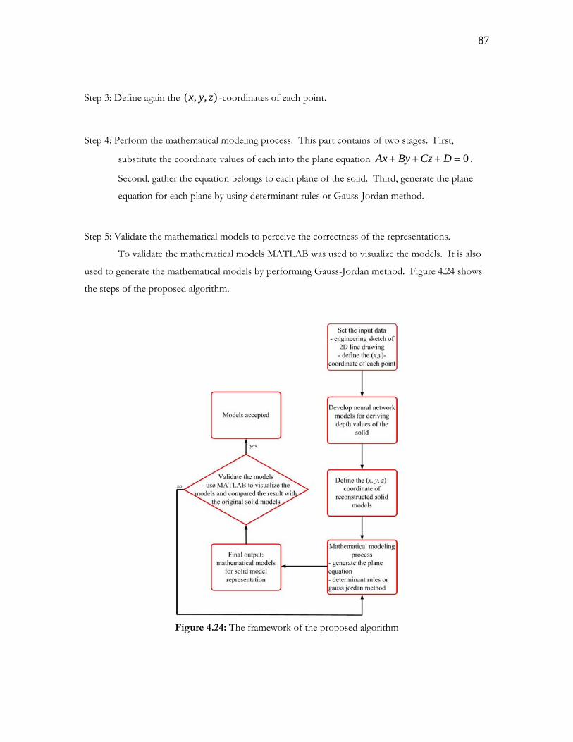
87
Step 3: Define again the ( , , )x y z -coordinates of each point.
Step 4: Perform the mathematical modeling process. This part contains of two stages. First,
substitute the coordinate values of each into the plane equation 0Ax By Cz D+ + + = .
Second, gather the equation belongs to each plane of the solid. Third, generate the plane
equation for each plane by using determinant rules or Gauss-Jordan method.
Step 5: Validate the mathematical models to perceive the correctness of the representations.
To validate the mathematical models MATLAB was used to visualize the models. It is also
used to generate the mathematical models by performing Gauss-Jordan method. Figure 4.24 shows
the steps of the proposed algorithm.
Figure 4.24: The framework of the proposed algorithm
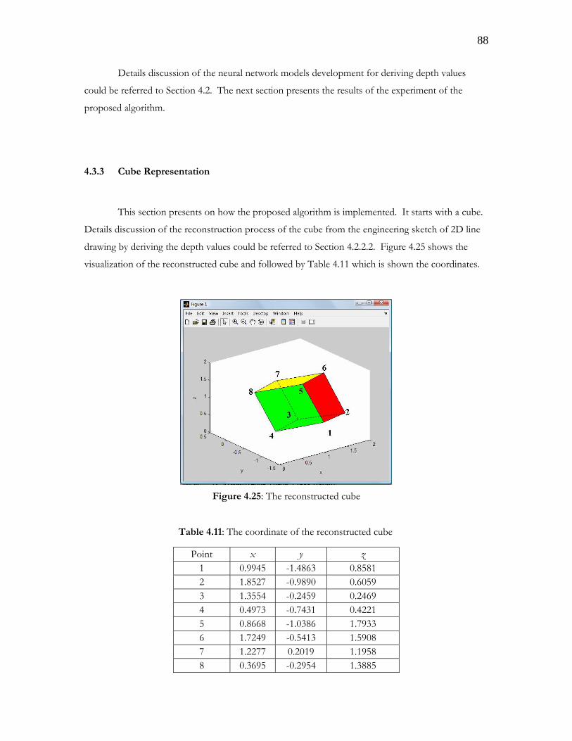
88
Details discussion of the neural network models development for deriving depth values
could be referred to Section 4.2. The next section presents the results of the experiment of the
proposed algorithm.
4.3.3 Cube Representation
This section presents on how the proposed algorithm is implemented. It starts with a cube.
Details discussion of the reconstruction process of the cube from the engineering sketch of 2D line
drawing by deriving the depth values could be referred to Section 4.2.2.2. Figure 4.25 shows the
visualization of the reconstructed cube and followed by Table 4.11 which is shown the coordinates.
Figure 4.25: The reconstructed cube
Table 4.11: The coordinate of the reconstructed cube
Point x y z 1 0.9945 -1.4863 0.8581 2 1.8527 -0.9890 0.6059 3 1.3554 -0.2459 0.2469 4 0.4973 -0.7431 0.4221 5 0.8668 -1.0386 1.7933 6 1.7249 -0.5413 1.5908 7 1.2277 0.2019 1.1958 8 0.3695 -0.2954 1.3885
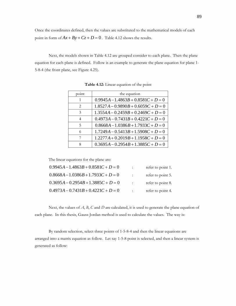
89
Once the coordinates defined, then the values are substituted to the mathematical models of each
point in form of 0Ax By Cz D+ + + = . Table 4.12 shows the results.
Next, the models shown in Table 4.12 are grouped consider to each plane. Then the plane
equation for each plane is defined. Follow is an example to generate the plane equation for plane 1-
5-8-4 (the front plane, see Figure 4.25).
Table 4.12: Linear equation of the point
point the equation 1 0.9945 1.4863 0.8581 0A B C D− + + = 2 1.8527 0.9890 0.6059 0A B C D− + + = 3 1.3554 0.2459 0.2469 0A B C D− + + = 4 0.4973 0.7431 0.4221 0A B C D− + + = 5 0.8668 1.0386 1.7933 0A B C D− + + =6 1.7249 0.5413 1.5908 0A B C D− + + =7 1.2277 0.2019 1.1958 0A B C D+ + + = 8 0.3695 0.2954 1.3885 0A B C D− + + =
The linear equations for the plane are:
0.9945 1.4863 0.8581 0A B C D− + + = : refer to point 1.
0.8668 1.0386 1.7933 0A B C D− + + = : refer to point 5.
0.3695 0.2954 1.3885 0A B C D− + + = : refer to point 8.
0.4973 0.7431 0.4221 0A B C D− + + = : refer to point 4.
Next, the values of A, B, C and D are calculated, it is used to generate the plane equation of
each plane. In this thesis, Gauss-Jordan method is used to calculate the values. The way is:
By random selection, select three points of 1-5-8-4 and then the linear equations are
arranged into a matrix equation as follow. Let say 1-5-8 point is selected, and then a linear system is
generated as follow:
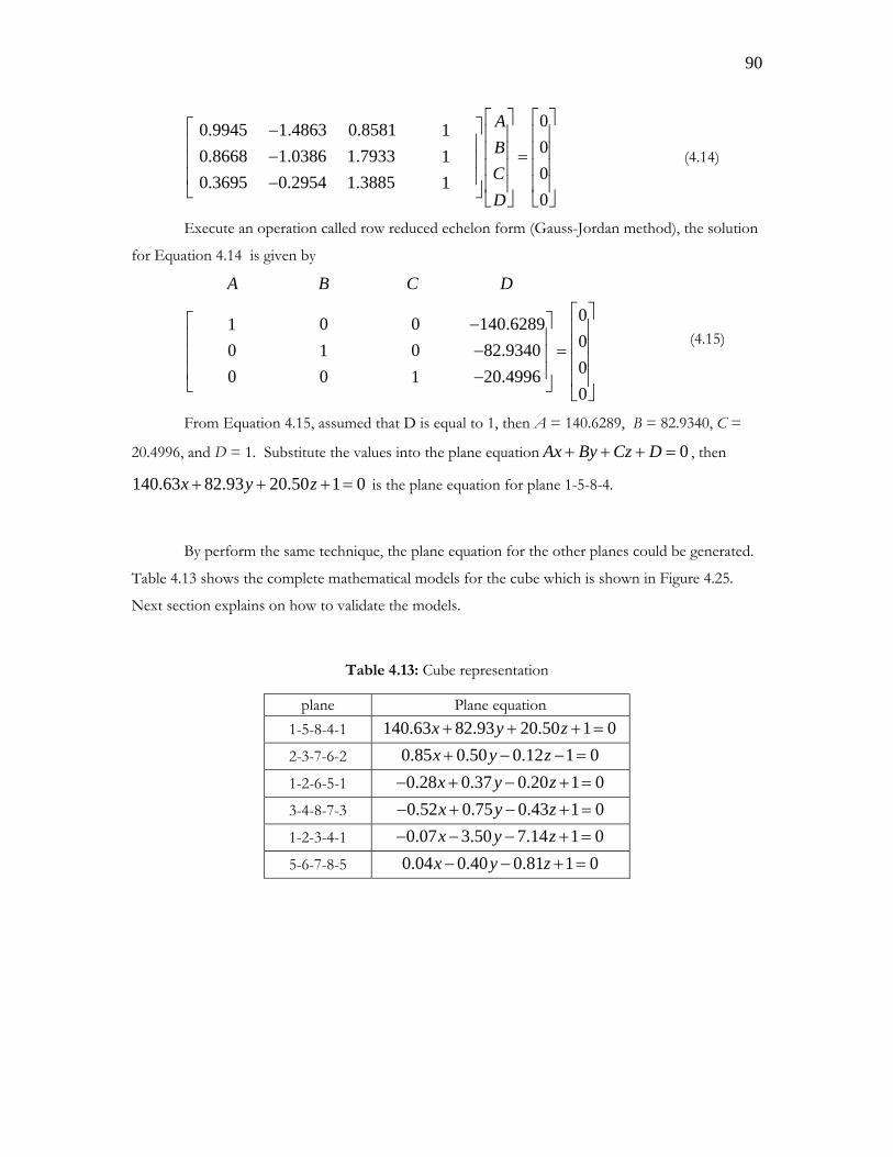
90
00.9945 1.4863 0.8581 100.8668 1.0386 1.7933 100.3695 0.2954 1.3885 10
ABCD
⎡ ⎤ ⎡ ⎤⎡ ⎤− ⎢ ⎥ ⎢ ⎥⎢ ⎥ ⎢ ⎥ ⎢ ⎥− =⎢ ⎥ ⎢ ⎥ ⎢ ⎥⎢ ⎥− ⎢ ⎥ ⎢ ⎥⎣ ⎦ ⎣ ⎦ ⎣ ⎦
(4.14)
Execute an operation called row reduced echelon form (Gauss-Jordan method), the solution
for Equation 4.14 is given by
00 0 140.6289100 0 82.9340100 0 20.499610
A B C D
⎡ ⎤⎡ ⎤− ⎢ ⎥⎢ ⎥ ⎢ ⎥− =⎢ ⎥ ⎢ ⎥⎢ ⎥− ⎢ ⎥⎣ ⎦ ⎣ ⎦
(4.15)
From Equation 4.15, assumed that D is equal to 1, then A = 140.6289, B = 82.9340, C =
20.4996, and D = 1. Substitute the values into the plane equation 0Ax By Cz D+ + + = , then
140.63 82.93 20.50 1 0x y z+ + + = is the plane equation for plane 1-5-8-4.
By perform the same technique, the plane equation for the other planes could be generated.
Table 4.13 shows the complete mathematical models for the cube which is shown in Figure 4.25.
Next section explains on how to validate the models.
Table 4.13: Cube representation
plane Plane equation 1-5-8-4-1 140.63 82.93 20.50 1 0x y z+ + + =
2-3-7-6-2 0.85 0.50 0.12 1 0x y z+ − − =
1-2-6-5-1 0.28 0.37 0.20 1 0x y z− + − + =
3-4-8-7-3 0.52 0.75 0.43 1 0x y z− + − + =
1-2-3-4-1 0.07 3.50 7.14 1 0x y z− − − + =
5-6-7-8-5 0.04 0.40 0.81 1 0x y z− − + =
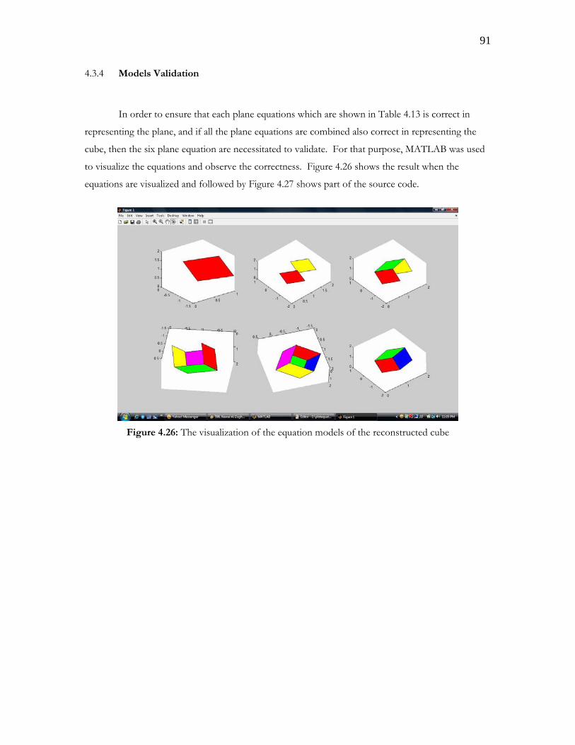
91
4.3.4 Models Validation
In order to ensure that each plane equations which are shown in Table 4.13 is correct in
representing the plane, and if all the plane equations are combined also correct in representing the
cube, then the six plane equation are necessitated to validate. For that purpose, MATLAB was used
to visualize the equations and observe the correctness. Figure 4.26 shows the result when the
equations are visualized and followed by Figure 4.27 shows part of the source code.
Figure 4.26: The visualization of the equation models of the reconstructed cube
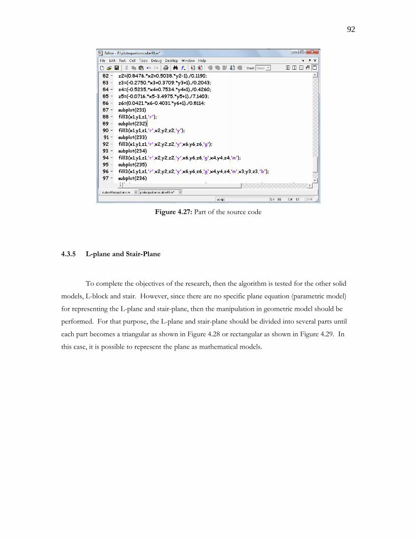
92
Figure 4.27: Part of the source code
4.3.5 L-plane and Stair-Plane
To complete the objectives of the research, then the algorithm is tested for the other solid
models, L-block and stair. However, since there are no specific plane equation (parametric model)
for representing the L-plane and stair-plane, then the manipulation in geometric model should be
performed. For that purpose, the L-plane and stair-plane should be divided into several parts until
each part becomes a triangular as shown in Figure 4.28 or rectangular as shown in Figure 4.29. In
this case, it is possible to represent the plane as mathematical models.
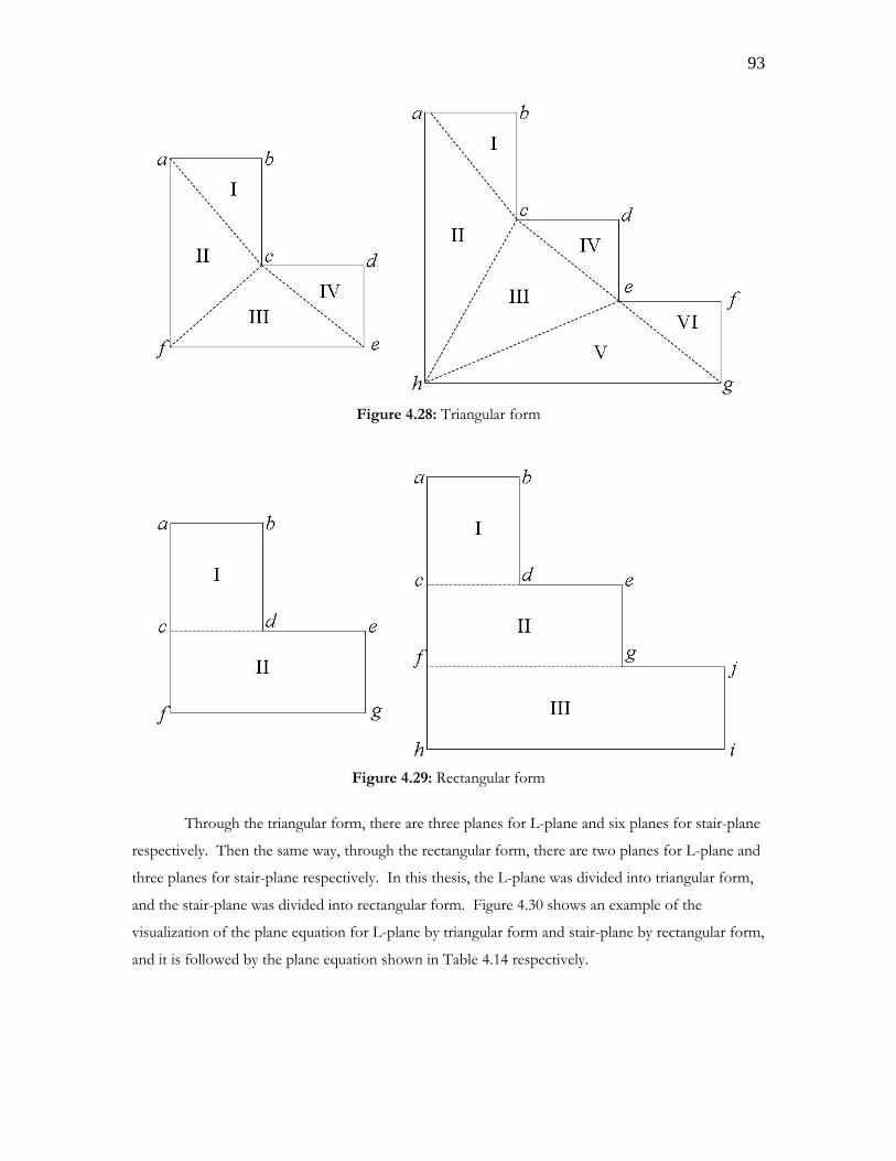
93
Figure 4.28: Triangular form
Figure 4.29: Rectangular form
Through the triangular form, there are three planes for L-plane and six planes for stair-plane
respectively. Then the same way, through the rectangular form, there are two planes for L-plane and
three planes for stair-plane respectively. In this thesis, the L-plane was divided into triangular form,
and the stair-plane was divided into rectangular form. Figure 4.30 shows an example of the
visualization of the plane equation for L-plane by triangular form and stair-plane by rectangular form,
and it is followed by the plane equation shown in Table 4.14 respectively.
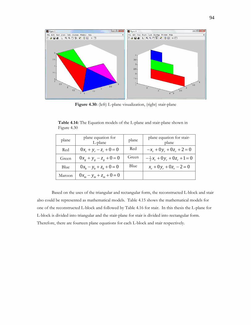
94
Figure 4.30: (left) L-plane visualization, (right) stair-plane
Table 4.14: The Equation models of the L-plane and stair-plane shown in Figure 4.30
plane plane equation for L-plane plane plane equation for stair-
plane Red 0 0 0r r rx y z+ − + = Red 0 0 2 0r r rx y z− + + + =
Green 0 0 0g g gx y z+ − + = Green 12 0 0 1 0r r rx y z− + + + =
Blue 0 0 0b b bx y z− + + = Blue 0 0 2 0r r rx y z+ + − =
Maroon 0 0 0m m mx y z− + + =
Based on the uses of the triangular and rectangular form, the reconstructed L-block and stair
also could be represented as mathematical models. Table 4.15 shows the mathematical models for
one of the reconstructed L-block and followed by Table 4.16 for stair. In this thesis the L-plane for
L-block is divided into triangular and the stair-plane for stair is divided into rectangular form.
Therefore, there are fourteen plane equations for each L-block and stair respectively.
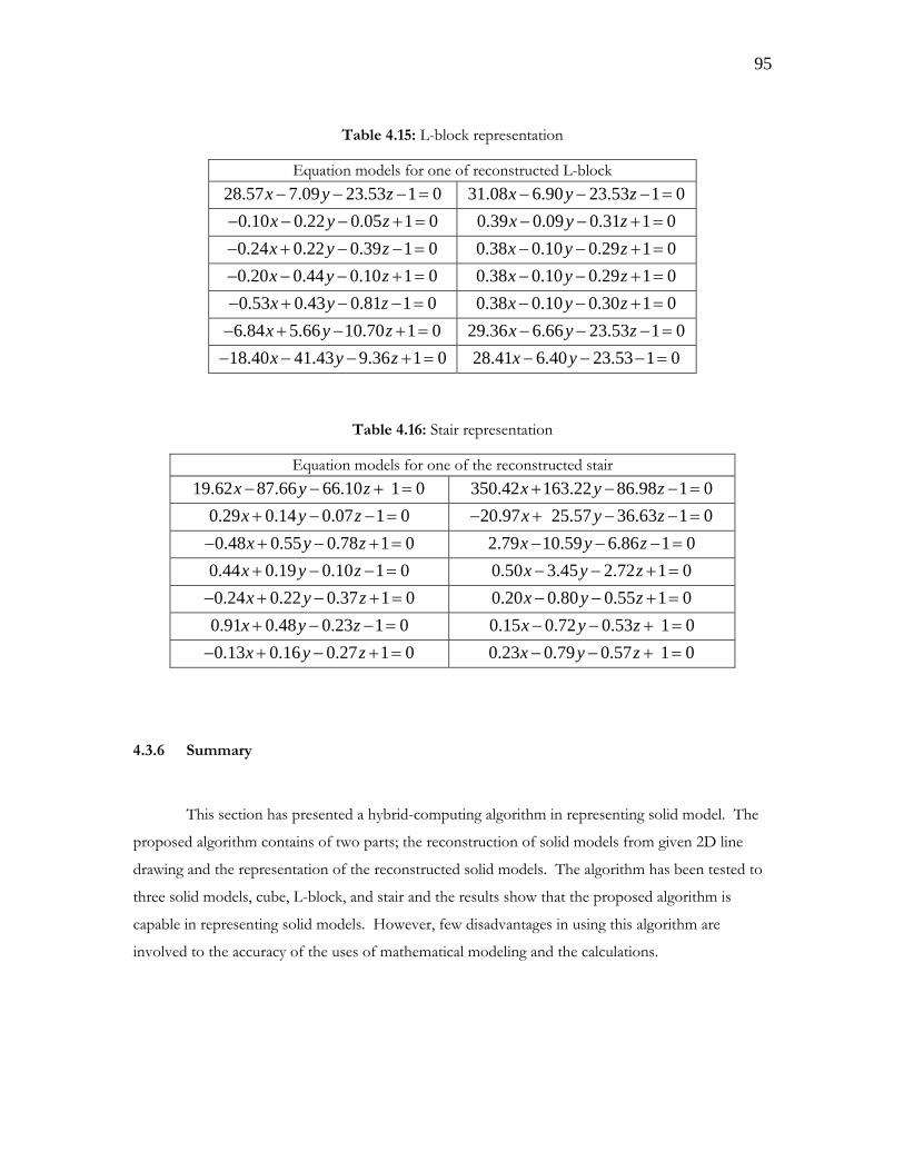
95
Table 4.15: L-block representation
Equation models for one of reconstructed L-block 28.57 7.09 23.53 1 0x y z− − − = 31.08 6.90 23.53 1 0x y z− − − =
0.10 0.22 0.05 1 0x y z− − − + = 0.39 0.09 0.31 1 0x y z− − + =
0.24 0.22 0.39 1 0x y z− + − − = 0.38 0.10 0.29 1 0x y z− − + =
0.20 0.44 0.10 1 0x y z− − − + = 0.38 0.10 0.29 1 0x y z− − + =
0.53 0.43 0.81 1 0x y z− + − − = 0.38 0.10 0.30 1 0x y z− − + =
6.84 5.66 10.70 1 0x y z− + − + = 29.36 6.66 23.53 1 0x y z− − − =
18.40 41.43 9.36 1 0x y z− − − + = 28.41 6.40 23.53 1 0x y− − − =
Table 4.16: Stair representation
Equation models for one of the reconstructed stair 19.62 87.66 66.10 1 0x y z− − + = 350.42 163.22 86.98 1 0x y z+ − − =
0.29 0.14 0.07 1 0x y z+ − − = 20.97 25.57 36.63 1 0x y z− + − − =
0.48 0.55 0.78 1 0x y z− + − + = 2.79 10.59 6.86 1 0x y z− − − =
0.44 0.19 0.10 1 0x y z+ − − = 0.50 3.45 2.72 1 0x y z− − + =
0.24 0.22 0.37 1 0x y z− + − + = 0.20 0.80 0.55 1 0x y z− − + =
0.91 0.48 0.23 1 0x y z+ − − = 0.15 0.72 0.53 1 0x y z− − + =
0.13 0.16 0.27 1 0x y z− + − + = 0.23 0.79 0.57 1 0x y z− − + =
4.3.6 Summary
This section has presented a hybrid-computing algorithm in representing solid model. The
proposed algorithm contains of two parts; the reconstruction of solid models from given 2D line
drawing and the representation of the reconstructed solid models. The algorithm has been tested to
three solid models, cube, L-block, and stair and the results show that the proposed algorithm is
capable in representing solid models. However, few disadvantages in using this algorithm are
involved to the accuracy of the uses of mathematical modeling and the calculations.
96
Bab 5 Kesimpulan & Cadangan ( Conclusion & Suggestion):
This chapter presents a conclusion for the research and ideas for further research. The
discussion starts with an introduction to the research achievements, research framework summaries,
research work summaries, and the contribution of the research. The discussion ends up with the
ideas for future works.
5.1 Introduction
Four contributions have been presented in this thesis. They are a new framework for solid
model reconstruction and representation, a new experimental data design, the developed neural
network models for deriving depth values and hidden point, and the hybrid-computing algorithm in
representing solid model. The developed research was started with the development of a new
framework and used 2D line drawing as the input data in the developing process to achieve the
objectives and to test it. They are sketches of three solid models, cube, L-block and stair which are
drawn on graph paper. By creating MATLAB program, the results also have been validated by
observing the accuracy and the similarity between the result that derived and the expected result.
In other hand, a new experimental data design has been developed to be used in the training,
validating and testing of neural network models, and it is also as one of the four contributions of the
research. Where other researches used moving average method (design in row) for the experimental
data design, in this research the data are design in column. However, using the design, the neural
network models are successful in recognizing the pattern of the data or in deriving depth values and
hidden point of solid model by given 2D line drawing, while the uses of moving average method are
not satisfied, in other words neural network models are probably not suitable in recognizing the data
pattern.
Few tools and literatures that are used in this research and provide to the contribution are
MATLAB 7.14, geometric analysis, affine transformation, and matrix theory that is made the
transformation process easy to do. As a conclusion, this research has successfully takes the
advantages of neural network with back propagation and mathematical modeling. It is also proving
the ability both of them in reconstructing and representing solid models from given 2D line drawing.
97
5.2 Research Framework Summary
This research has been started with the discussion of few literature reviews on solid model,
issues on that and the problem that have been identified, and few previous works that are related
considering to the issues. And then, step forward to the conclusion about the research focus and the
objectives of the research. However, few assumptions and limitations have been made to simplify
the research works.
After make clear about the research focus and objectives, then the research starts to create
the methodology of the research, develop the framework that covered all the parts of the research,
and then develop any techniques that are used to solve the problems and to achieve the objectives of
the research. On the research development, the process has been started with the creation of the
nature data, data extraction, and data expansion then followed by designing the data. In this stage,
the data are ready to use. And then, neural network models are developed in order it can be used to
derive depth values and hidden point of solid model. Three solid models from given 2D line
drawing have been tested and the results showed that neural network models are capable in
reconstructing the solid by deriving the depth values and hidden point. In this stage, the research
was successful in reconstructing solid model from given 2D line drawing.
Then the research is continued to the development of hybrid-computing algorithm in
representing solid model. In this stage, the results from the previous stage employed and combined
with mathematical modeling to represent the reconstructed solid based on surface-based model as
mathematical models. This kind of representations is also known as parametric scheme
representation, which is used explicit or implicit function.
The result analyses also have been done by making direct comparison among the results to
the expectation and to few previous works. Some of them are work by Peng and Shamsuddin
(2004), Haron (2004), Subri (2006), and Matondang et al. (2006). Figure 5.1 shows simple schematic
of the research framework.
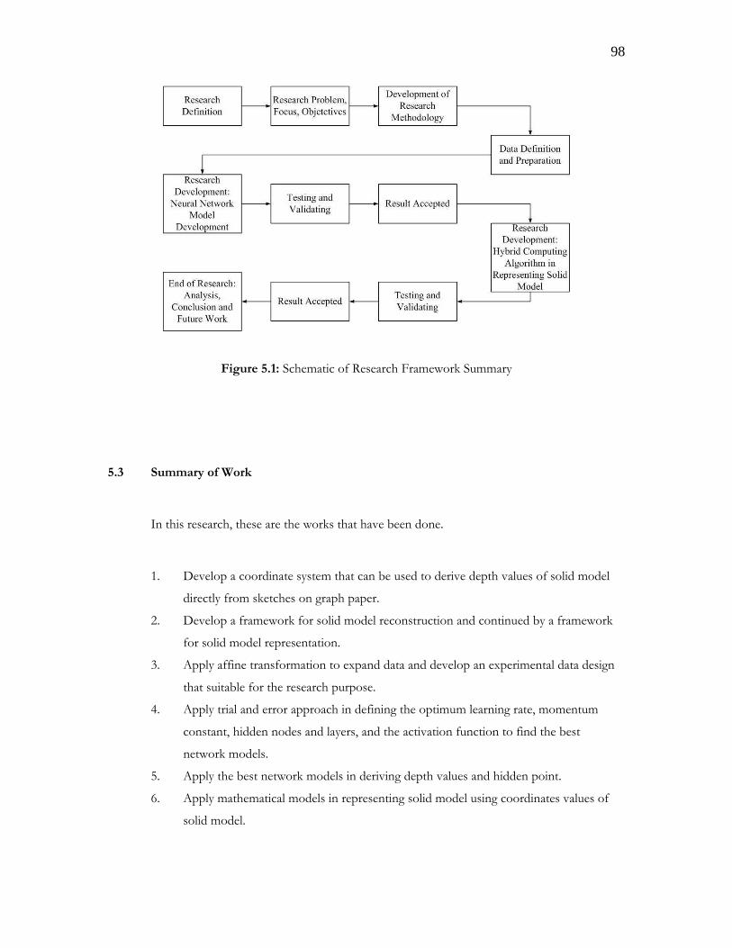
98
Figure 5.1: Schematic of Research Framework Summary
5.3 Summary of Work
In this research, these are the works that have been done.
1. Develop a coordinate system that can be used to derive depth values of solid model
directly from sketches on graph paper.
2. Develop a framework for solid model reconstruction and continued by a framework
for solid model representation.
3. Apply affine transformation to expand data and develop an experimental data design
that suitable for the research purpose.
4. Apply trial and error approach in defining the optimum learning rate, momentum
constant, hidden nodes and layers, and the activation function to find the best
network models.
5. Apply the best network models in deriving depth values and hidden point.
6. Apply mathematical models in representing solid model using coordinates values of
solid model.
99
5.4 Contributions
Basically, five contributions have been produced during the research sessions. Four of them
are successful achieved the objectives, and another one was failed. This section presents the
summaries of each of them. Start with the failed one, namely the new coordinate system. In the
early beginning of the research, the author of this thesis was planned to derive depth values of solid
model directly from the sketch on graph paper. However, by doing few investigation, it is impossible
to draw the standard 3D coordinate system, then draw solid model in the above of the coordinate
system, then derive the coordinate even if just the x and y values (unless the coordinates was given
then the solid drawn). Therefore, the author attempts to devise a new coordinate system that makes
it possible. As a result, a new coordinates system that used right hand method was obtained.
Unfortunately, the coordinates system failed in shielding the robustness of the solid even if it is
successful in deriving the coordinates of each point of the sketch. Causing of the weaknesses, the
developed coordinates system could not be used. Therefore, the standard coordinate system is used
in that way during the research.
Due to the unsuccessful of the coordinate system in deriving depth values of solid model,
then neural network is employed and developed to derive depth and also hidden point of solid
models. However, it was successful and there are six neural network models have been produced as
the best models, and then they are tested to three solid models from given 2D line drawing. Based
on the experimental data results and the analysis of the accuracy of the derivation, it can be
concluded that the developed neural network models are capable and successful in reconstructing
solid model by deriving depth values and hidden point.
In conjunction with the development process of neural network models, an alternative
technique for the experimental data design also produced. This technique designed the data in
column, while others related previous works designed the data in row. However, the use of the
developed design is much better than the use of moving average method, and it has been proven by
the results.
With the successful of neural network models in deriving both of depth values and hidden
point, then the results are employed as the input to develop and use mathematical models in
representing solid model. The coordinates of the reconstructed solid models are used to generate the
100
representation of the solid based on surface-based model. In this stage, the reconstructed solid
models are represented as mathematical models.
Three sketches of solid model in form of 2D line drawing have been used to develop and
test the proposed neural network models and the proposed algorithm. The experimental results
shows that this research was successful in reconstructing and representing solid model from given
2D line drawing.
5.5 Future Works
The following are some of the ideas that can be used as future works for further research.
1. This research has tried to develop a coordinate system that can be used to derive the
depth values of solid model directly from the sketch, but failed with it. Any
suggestions and manipulation on geometrical modeling could make this things right.
2. This research take times in set up the network and finding the optimum parameters
value, use other evolutionary methods such genetic algorithm (GA) should be realized
to cut the time uses and reduced the uses of data for training and validating.
3. There is no curve involved in the solid model that has been tested. Therefore, use
other type of solid model can be realized in other to see the capable of the proposed
algorithm in reconstructing regular and irregular solid models.
4. Further research in obtaining the training patterns for the network training can be
realized to produce robust training patterns.
5. Finding the exact plane equation for L-plane and stair-plane can be realized to reduce
the number of models in representing solid models, and make it simpler.
101
Rujukan (References):
Barhak, J. and Fischer, A. (2001). Adaptive Reconstruction of Freeform Objects with 3D SOM
Neural Network Grid. Proceeding of The 9th Pacific Conference on Computer Graphics and Applications.
Tokyo – Japan: IEEE, 97-195.
Barr, A. H. (1984). Local and Global Deformations of Solid Primitives, Computer Graphics. 18(3).
Bross, I. (1972). Scientific Strategies in Human Affairs: Use of Deep Mathematical Models.
Transactions of the New York Academy of Sciences. 34(3). 187-199.
Christos, S., and Dimitrios, S. (1996). Neural Network. SURPRISE 96 JOURNAL. Quen’s Gate-
London. 4.
Clowes, M. (1971). On Seeing Things. Artificial Intelligence. 2(1). 79 - 112.
Cretu, A. -M. (2003) 3D Object Modeling-Issues and Technique. PhD Thesis. University of Ottawa.
Cretu, A. –M., Petriu, E. M., and Patry, G. G. (2003). Neural Network Architecture for 3D Object
Representation. Proceedings. The 2nd IEEE Internatioal Workshop on Haptic, Audio and Visual
Environments and Their Applications, 2003. HAVE 2003. 31- 36.
Eykhoff, P. (1974). System Identification. J. Wiley, London.
Fausett, L. V. (1994). Fundamentals of Neural Networks: Architectures, Algorithms and Applications. N. J.:
Prentice-Hall.
Fayolle, P. A., Rosenberger, C., and Toinard, C. (2004). 3D Shape Reconstruction of Template
Models Using Genetic Algorithms, Proceeding of 17th International Conference on Pattern Recognition.
Cambridge – UK: IEEE. 269-272.
Foley, J. D., Van Dam A., and Feiner, S. K. (1996). Computer Graphics Principles and Practice. New York.:
Addison-Wesley.
Freeman, H. (1969). On the Quantization of Line Drawing Data, IEEE Trans. System Science and
Cybern. SSC-5(1). 70-79.
Fu, L. M. (1994). Neural Networks in Computer Intelligence. McGraw-Hill Book, Inc. Singapore
Fukui, Y. (1988). Input Method of Boundary Solid by Sketching. Computer Aided Design. 20(8). 434 –
440.
Grimstead, J., and Martin, R. R. (1995). Creating Solid Model From Single 2D Sketches, Proceedings
Third Symp. On Solid Modeling Applications, ACM SIGGRAPH. 323-337.
Haron, H. (2004). Enhanced Algorithms for Three-Dimensional Object Interpreter. PhD Thesis. University
Technology Malaysia.
Haykin, S. (1999). Neural Networks: A Comprehensive Foundation, Upper Saddle River, Nj: Prentice-Hall.
Hebb, D. O. (1949). The Organization of Behavior. A Neuropsychological Theory. Wiley-New York.
102
Heyden, A. (1995). Geometry and Algebra of Multiple Projective Transformation, Dept. of Mathematics,
Lund University, Sweden.
Huffman, D. A. (1971). Impossible Objects as Nonsense Sentences. Machine Intelligence. Edinburgh
University Press. 295-323.
Idesawa, M. (1973). A System to Generate a Solid Figure from Three Views, Bulletin of JSME. 216-
225.
Junior, Ad.M.B., Neto, A.D.D., and de Melo, J.D. (2004). Surface Reconstruction Using Neural
Networks and Adaptive Geometry Meshes. Neural Networks, 2004. Proceedings. 2004 IEEE
International Joint Conference on. 803-807.
Kanade, T. (1980). A theory of Origami world. Artificial Intelligence. 13. 279 - 311.
Lamb, D., and Bandopadhay, A. (1990). Interpreting a 3D Object from a Rough 2D Line Drawing.
Proceeding of Visualization '90. 59 - 66.
Leclerc, Y. G., and Fiscler, M. A. (1992). An Optimization Based Approach to the Interpretation of
Single Line Drawings as 3D Wire Frames. International Journal of Computer Vision. 9(2). 113 –
136.
Lim, K.T., and El-Mounayri, H. (1999). CAD/CAM-based geometric modeling simulation for
virtualmanufacturing. Electrical Insulation Conference and Electrical Manufacturing & Coil Winding
Conference. 547-551.
Lipson, H. and Shpitalni, M. (1996). Correlation-Based Reconstruction of a 3D Object from a Single
Freehand Sketch. International Proceeding AAAI Spring Symposium Series--Sketch Understanding. Palo,
Alto, USA. 99-104.
Mackworth, A. K. (1973). Interpreting Pictures of Polyhedral Scenes. Artificial Intelligence. 4. 121-137.
Marill, T. (1991). Emulating the Human Interpretation of Line-Drawings as Three- Dimensional
Objects. International Journal of Computer Vision. 6(2). 147- 161.
Matondang, M. Z., Haron, H., and Talib, M.S., (2006). Three-Dimensional Visualization of Two-
Dimensional Data: The Mathematical Modeling, Proceedings of the 2nd IMT-GT Regional Conference
on Mathematics, Statistics and Applications, 13-15 June 2006, Penang, Malaysia. Vol. 4: Computer
Sciences and Applications. Ed. by Yahya Abu Hassan, Adli Mustafa and Zarita Zainuddin, 79-87.
Mortenson, M. E. (1997). Geometric Modeling, Second Edition, Wiley Computer Publishing.
Moussa, A. S. (2003). The Implementation of Intelligent QoS Networking by the Development and
Utilization of Novel Cross-Disciplinary Soft Computing Theories and Techniques. PhD
Thesis. The Florida State University College of Arts and Sciences.
Negnevitsky, M. (2005). Artificial Intelligence, A Guide to Intelligence Systems. 2nd Edition.
Eidenberg-England.: Addison-Wesley.
103
Ovaska, S. J., Kamiya, A., and Chen, Y. Q. (2006). Fusion of soft computing and hard computing:
Computational structures and characteristic features. IEEE Transactions on Systems, Man, and
Cybernetics-Part C: Applications and Reviews. 36(3). 439 - 448.
Ovaska, S. J., Dote, Y. Furuhashi, T., Kamiya, A., and VanLandingham, H.F. (1999). Fusion of Soft
Computing and Hard Computing Techniques: A Review of Applications. Systems, Man, and
Cybernetics, 1999. IEEE SMC '99 Conference Proceedings. 1999 IEEE International Conference on.
1. 370 - 375.
Peng, L. W., and Shamsuddin, S. M. (2004). 3D Object Reconstruction and Representation Using
Neural Networks. Association for Computing Machinery, Inc. 139-147.
Piperakis, E., and Kumazawa, I. (2001). Affine Transformations of 3D Objects Represented with
Neural Networks. IEEE. 213 – 223.
Requicha, A. A. G. (1980). Representation for Rigid Solid: Theory, Methods, and System, ACM
Computing Surveys. 12(4). 437- 464.
Requicha, A. A. G., and Rossignac, J. R. (1992). Solid Modeling and Beyond. IEEE Computer Graphics
& Application. (Special Issue on CAGD). 12(5). 31- 44.
Rossignac, J. R., and Requicha, A. A. G. (1999). Solid Modeling. Wiley Encyclopedia of Electrical and
Electronics Engineering. Published online. 1-17.
Sallehuddin, R., Ngadiman M. S., and Shamsuddin, S. M. (2000). Peramalan Siri Masa Variasi
Bermusim-Satu Pendekatan Alternatif Menggunakan Rangkaian Neural. Proceeding of the National
Conference on Management Science/ Operational Research. 1. 32-37.
Samadzadegan, F., Azizi, A., Hahn, M., and Lucas, C. (2005). Automatic 3D Object Recognition and
Reconstruction Based on Neuro-Fuzzy Modeling. ISPRS Journal of Photogrammetry & Remote
Sensing 59. 255-257.
Shapiro, V. (2002). Solid Modeling. Handbook of Computer Aided Geometric Design, (G. Farin, J.
Hoschek, M.-S. Kim, eds.). Elsevier Science Publishers. 473 – 518.
Shah, J. J., Dedhia, H., Pherwani, V., Solkhan, S. (1997). Dynamic Interfacing f Applications to
Geometric Modeling Services via Modeler Neutral Protocol. lsevier Computer-Aided Designi. 29.
811-824.
Shepherd, G.M., and Koch, C. (1990). Introduction to Synaptic Circuits. In G.M. Shepherd (ed.) The
Synaptic Organization of the Brain. Oxford University Press, New York. 3 - 31.
Shum, Simon Siu-pun. (1999). Solid Reconstruction from Orthographic Projected Line Drawing, PhD Thesis.
Department of Mechanical Engineering and Aeronautics.
Subri, S. H. (2006). Aplikasi Rangkaian Neural dalam Pengesan Simpang BagiPenterjemah Lakaran Pintar,
(Neural Network Applied on Corner Detection for an Intelligent of Sketch Intepreter). Master
Thesis Universiti Teknologi Malaysia.
104
Sugihara, K. (1986). Machine Interpretation of Line Drawings. The MIT Press.
Suhterland, I.E. (1963). Sketchpad A Man-Machine Graphical Communication System, Proceeding
AFIPS Conference Spring Joint Computer Conference. 23. 329-346.
Turner, A., Chapman, D., and Penn, A. (2000). Sketching Space. Computers and Graphics, Special Issue on
Calligraphic Interfaces. Vol. 24(6). pp. 869–879.
Wani, S. (2004). 3D Reconstruction of Architectural Scene from Single 2D Perspective Sketches,
Master Thesis, The University of Texas Arlington.
Wang, W. (1992). On The Automatic Reconstruction of a 3D Object’s Constructive Solid Geometry Representation
From Its 2D Projection Line Drawing. PhD Thesis, University of Massachusetts-Lowell, University
of Massachusetts.
Wang, W., and Grinstein, G. (1989). A Polyhedral Object's CSG-Rep Reconstruction from a Single
2D Line Drawing. Proceedings of 1989 SPIE Intelligent Robots and Computer Vision III: Algorithms
and Techniques. 1192. 230 -238.
Wei, X. (1987). Computer Vision Method for 3D Quantitative Reconstruction from a Single Line Drawing. PhD
Thesis. Department of Mathematics. Beijing University. China (in Chinese; for a review in
English see Wang and Grinstein, 1993).
Yan Tangy., Wen-jing Chen., Xian-yu Sua, and Li-qun Xiang. (2007). Neural Network Applied to
Reconstruction of Complex Objects Based on Fringe Projection. Journal of Optics Communication
278. 274-278.
Zadeh, L. A. (1993). Fuzzy Logic and Softcomputing. Plenary Speaker, Proceedings of IEEE International
Workshop on Neuro Fuzzy Control. Muroran, Japan.
Zadeh, L. A. (1996). The Role of Soft Computing and Fuzzy Logic in the Conception, Design,
Development of Intelligent Systems. Plenary Speaker, Proceedings of the International Workshop on
soft Computing Industry. Muroran, Japan.
Zadeh, L. A. (1999). From Computing with Numbers to Computing with Words--from Manipulation
of Measurements to Manipulation of Perceptions. IEEE Transactions on Circuits and Systems. 45.
105 - 119.
Zeid, L. (1991). CAD/CAD Theory and Practice. Mcgraw-Hill, Inc. USA.