DETERMINATION OF COEFFICIENT OF RATE OF HORIZONTAL CONSOLIDATION OF PEAT SOIL

NURLY GOFAR

Laporan Projek Penyelidikan Fundamental Vot 75210

Faculty of Civil Engineering Universiti Teknologi Malaysia

JUNE 2006

ii

IN THE NAME OF ALLAH THE BENEFICENT THE MERCIFUL.

ACKNOWLEDGEMENT

The author would like to convey her sincere appreciation to the Research

Management Center (RMC) of Universiti Teknologi Malaysia for the support to

carry out this fundamental research (vot 75210). Special gratitude is dedicated to the

Faculty of Civil Engineering and the staff of the Geotechnical Laboratory for their

support and encouragement. The author is also indebted to her research assistants

(Yulindasari and Wong Leong Sing) for conducting the laboratory work and analysis.

Appreciations are also conveyed to those who contributed in one way or the other to

finish this research.

iii

ABSTRACT

Encountered extensively in wetlands, fibrous peat is considered as problematic soil because it exhibits unusual compression behavior. When a mass of fibrous peat soil with both vertical and horizontal drainage boundaries is subjected to a consolidation pressure, rate of excess pore water dissipation from the soil in the horizontal direction (ch) is expected to be higher than that in the vertical direction (cv). ch/cv of two is commonly used in practice for estimation of consolidation in soft clay improved by vertical drain whereas published data showed that the ch/cv ratio for fibrous peat could be as high as 300.

This research focused on the consolidation behavior of fibrous peat from

Kampung Bahru, Pontian, Johor with respect to one-dimensional vertical and horizontal consolidation. The result is useful for evaluation of the utilization of some type of vertical drainage for soil improvement to accelerate the settlement of fibrous peat soil.

Results from constant head permeability reveal that the soil is almost

isotropic as indicated by equal initial permeability in horizontal and vertical direction. Hydraulic consolidation tests in Rowe cell, the coefficient of rate of horizontal consolidation increases significantly with consolidation pressure, while the increase in the coefficient of rate of vertical consolidation does not increase as much. The ch/cv ratio increase from 3.5 to 6 for consolidation pressure of 25 to 200 kPa. The ratio of coefficient of permeability kh/kv under a consolidation pressure of 200 kPa is about 5. This finding implies that the utilization of horizontal drain maybe suitable for accelerating settlement and reducing the effect of secondary consolidation.

iv

ABSTRAK

Ditemui secara meluas di kawasan paya, tanah gambut gentian adalah tanah bermasalah kerana mempunyai sifat pengukuhan yang luar biasa. Apabila sesuatu jisim tanah gambut berfiber yang terdedah kepada sistem saliran air secara menegak dan mendatar dikenakan tekanan pengukuhan, kadar lesapan air terlebih secara mendatar (ch) pada amnya adalah lebih tinggi berbanding dengan kadar lesapan air terlebih secara menegak (cv). Nisbah ch/cv sebesar dua biasa digunakan untuk pengiraan pengukuhan tanah liat lembut yang dibaiki dengan menggunakan saliran menegak. Bahkan data yang sudah dipublikasikan sebelum ini menunjukkan bahawa nisbah tersebut dapat meningkat sehingga 300 untuk tanah gambut gentian.

Projek penyelidikan ini membincangkan hasil kajian makmal tentang sifat

pengukuhan tanah secara menegak dan mendatar bagi sampel-sampel tanah gambut gentian yang didapati dari kampung Bahru, Pontian, Johor. Hasil kajian akan berguna untuk mengevaluasi kesesuaian kaedah saliran menegak untuk pembaikan tanah gambut gentian.

Keputusan ujian keboleh telapan dengan tekanan tetap yang ditunjukkan dari

cirri keboleh telapan menegak (kv) dan mendatar (kh) menunjukan bahawa tanah adalah isotropik. Walau bagaimanapun ciri keboleh telapan ini berkurang selepas berlakunya tekanan. Keputusan ujian pengukuhan hidraulik dengan sel Rowe menunjukkan bahawa ciri keboleh telapan dalam arah mendatar meningkat dengan cepat berbanding tekanan pengukuhan. Nisbah ch/cv meningkat dari 3.5 kepada 6 untuk peningkatan tekanan pengukuhan dari 25 kepada 200 kPa. Nisbah kh/kv adalah 5 untuk tekanan pengukuhan sebesar 200 kPa. Ini menandakan bahawa penggunaan sistem saliran air secara mendatar mungkin sesuai bagi mempercepatkan proses pemendapan tanah gambut gentian.

v

TABLE OF CONTENTS

CHAPTER

TITLE

PAGE

1

ACKNOWLEDGEMENT ABSTRACT ABSTRAK TABLE OF CONTENTS LIST OF TABLES LIST OF FIGURES LIST OF SYMBOLS LIST OF APPENDICES INTRODUCTION

ii iii iv v

viii ix

xiii xv 1

1.1 1.2 1.3

Background Objectives of Study Scope of Study

1 2 3

2 LITERATURE REVIEW

4

2.1 Fibrous Peat 4

2.1.1 Definition 4 2.1.2 Structural Arrangement 5 2.1.3 Physical and Chemical Properties 7 2.1.4 Engineering Properties 8 2.1.5 Permeability 10

2.2 Soil Compressibility 12

2.2.1 Primary Consolidation 12 2.2.2 Secondary Compression 18

2.3 Large Strain Consolidation Test 20 2.3.1 Problems Related to Conventional Test 20 2.3.2 Large Strain Test (Rowe Cell) 22

2.4 Analysis of Time-Compression Curve 25

2.5 Measurement of Horizontal Coefficient of Consolidation

32

vi

3

METHODOLOGY 33

3.1 Introduction 33

3.2 Preliminary Tests 35 3.3 Large Strain Consolidation Test 35 3.4 Data Analysis 36 3.4.1 Analysis of Test Results 36 3.4.2 Analysis of Time-Compression Curve 37 3.4.3 Analysis of Output 38

4 RESULTS AND DISCUSSION

39

4.1 Introduction 39 4.2 Soil Identification 40

4.3 Fiber Orientation 42 4.4 Analysis of Compression Curves from Consolidation

Tests (Rowe Cell) 44

4.5 Effect of Secondary Compression on Rate of Consolidation

53

4.6 Permeability 56 4.6.1 Initial Permeability 57

4.6.2 Effect of Consolidation Pressure in Permeability

58

4.6.3 Coefficient of Permeability based on Consolidation Test

59

4.7 Discussion

62

5 CONCLUSIONS AND RECOMMENDATION FOR FUTURE STUDY

66

5.1

5.2

Conclusions

Recommendation For Future Study

66

67

REFERENCES

68

Appendices A – F

71

vii

LIST OF TABLES

TABLE NO. TITLE

PAGE

4.1 Basic properties of the peat soil

40

4.2 Average time for completion of primary consolidation (t100) obtained from Rowe test results

49

4.3 Average coefficient of consolidation obtained from Rowe test results

52

4.4 Average degree of consolidation (U%) and the time for the beginning of secondary compression (tp) obtained from Rowe test results

54

4.5 Effect of consolidation pressure on coefficient of permeability

59

4.6 Coefficient of volume compressibility mv

60

4.7 Coefficient of permeability based on hydraulic consolidation test

60

4.8 Compressibility parameters obtained from consolidation tests with vertical and horizontal drainage (under consolidation pressure of 100 kPa, if applicable)

63

viii

LIST OF FIGURES

FIGURE NO. TITLE PAGE 2.1

Schematic diagram of (a) deposition and (b) multi-phase system of fibrous peat (Kogure et al., 1993)

6

2.2 Scanning Electron Micrographs of Middleton fibrous peat; (a) horizontal plane, (b) vertical plane (Fox and Edil, 1996)

7

2.3

Coefficient of permeability versus void ratio for vertical and horizontal specimens of Portage peat (Dhowian and Edil, 1980)

11

2.4 Plot of Void ratio vs. pressure in linear scale

14

2.5

Plot of void ratio vs. pressure in logarithmic scale

14

2.6

Consolidation curve for two-way vertical drainage (Head, 1982)

16

2.7

Determination of cv by Cassagrande method

17

2.8

Determination of cv by Taylor method

18

2.9

Determination of the coefficient of rate of secondary compression from consolidation curve (Cassagrande)

19

2.10

Schematic diagram of Oedometer Cell 21

2.11

Schematic diagram of Rowe Consolidation cell

22

2.12

Drainage and loading conditions for consolidations tests in Rowe cell: (a),(c), (e), (g) with ‘free strain’ loading, (b), (d), (f), (h) with ‘equal strain’ loading (Head, 1986)

24

ix

2.13

Types of time-compression curve derived from consolidation test (Leonards and Girault, 1961)

25

2.14

(a) Time-compression curves, and (b) time-degree of consolidation from the measured pore water pressure dissipation curves for peat (Robinson, 2003)

27

2.15

Degree of consolidation from the pore water pressure dissipation curves plotted against compression for several consolidation data for peat (Robinson, 2003)

28

2.16

(a) Time-total settlement curves for peat and (b) Time-settlement curve after removing the secondary compression (Robinson, 2003)

30

2.17

Primary consolidation versus log time curve for evaluation of coefficient of consolidation

31

2.18 Secondary compression versus log time curve for evaluation of coefficient of secondary consolidation

31

3.1 Flow chart of the study

34

3.2 Rowe Consolidation cell 36

4.1 Typical log time-compression curves from oedometer test

41

4.2 SEM of Fibrous Peat Samples at initial state (a) Vertical Section x400, (b) Horizontal Sectionx400

43

4.3 SEM of Fibrous Peat Samples under consolidation Pressure of 200 kPa (a) Vertical Section x400 (b) Horizontal Section x400

43

4.4 Log time-compression curves from hydraulic consolidation test with vertical drainage for consolidation pressure 50 kPa

45

4.5

Log time-pore water pressure curve from hydraulic consolidation test with vertical drainage for consolidation pressure 50 kPa

45

4.6 Log time-compression curves from hydraulic consolidation test with horizontal drainage for consolidation pressure 50 kPa

46

x

4.7 Log time-pore water pressure curve from

hydraulic consolidation test with horizontal drainage for consolidation pressure 50 kPa

46

4.8 Typical degree of consolidation - compression curve from hydraulic consolidation test with two-way vertical drainage

48

4.9 Typical degree of consolidation - compression curve from hydraulic consolidation test with horizontal drainage

48

4.10 Variation of the beginning of secondary consolidation with consolidation pressure for sample tested under vertical consolidation

50

4.11 Variation of the beginning of secondary consolidation with consolidation pressure for sample tested under horizontal consolidation

50

4.12 Variation of coefficient of secondary consolidation with consolidation pressure for sample tested under vertical51 consolidation

51

4.13 Variation of coefficient of secondary consolidation with consolidation pressure for sample tested under horizontal consolidation

51

4.14 Variation of the beginning of secondary consolidation with consolidation pressure for sample tested under vertical consolidation

53

4.15 Variation of the beginning of secondary consolidation with consolidation pressure for sample tested under horizontal consolidation

54

4.16 Variation of coefficient of secondary consolidation with consolidation pressure for sample tested under vertical consolidation

55

4.17 Variation of coefficient of secondary consolidation with consolidation pressure for sample tested under horizontal consolidation

56

4.18 Graph of coefficient of permeability at standard temperature of 20°C, ko (20°C) versus initial void ratio, eo of the fibrous peat soil samples

58

xi

4.19 Relationship between Vertical Coefficient of

Permeability and Consolidation Pressure obtained from all tests

61

4.20 Relationship between Horizontal Coefficient of Permeability and Consolidation Pressure obtained from all tests.

61

xii

LIST OF SYMBOLS

A - Area of sample

AC - Ash content

B - Pore pressure parameter

cc - Compression index

ch - Horizontal coefficient of consolidation

cr - Recompression index

cv - Vertical coefficient of consolidation

cα, cα1 - Coefficient of secondary compression

cα2 - Coefficient of tertiary compression

D - Diameter of sample

e - Void ratio

eo - Initial void ratio

FC - Fiber content

Gs - Specific gravity

H, Ho - Initial thickness of consolidating soil layer

h - Head loss due to the height of water in the burette

i - Hydraulic gradient

kh - Horizontal coefficient of permeability

kho - Initial horizontal coefficient of permeability

kv - Vertical coefficient of permeability

kvo - Initial vertical coefficient of permeability

xiii

L - Longest drainage path in consolidating soil layer; equal to half of H with top and bottom drainage, and equal to H with top drainage only

m - Secondary compression factor

mv - Coefficient of volume compressibility

OC - Organic content

p - Consolidation pressure

po - Initial pressure

p1 - Inlet pressure

p2 - Outlet pressure

Q - Cumulative flow

q - Rate of flow

r - Radius of sample

Tr - Radial theoretical time factor

Tv - Vertical theoretical time factor

t - Time

ts - Time to reach end of secondary compression

tp - Time to reach end of primary consolidation

Ur - Average degree of consolidation due to radial drainage

Uv - Average degree of consolidation due to vertical drainage

u - Excess pore water pressure at any point and any time

uo - Initial excess pore water pressure

w - Natural moisture content

∆Hs - Change in height of soil layer due to secondary compression from time, t1 to time, t2

∆Ht

-

Change in height of soil layer due to tertiary compression from time, t3 to time, t4

xiv

∆p - Pressure difference

εi - Instantaneous strain

εp - Primary strain

εs - Secondary strain

εt - Tertiary strain

γw - Unit weight of water

σ'v - Effective vertical stress

δ - Total compression

δp - Primary consolidation settlement

δs - Secondary compression

xv

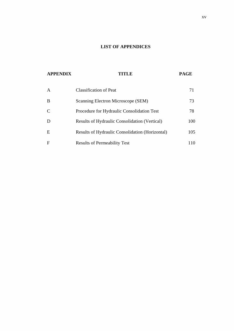
LIST OF APPENDICES

APPENDIX TITLE PAGE

A

Classification of Peat 71

B Scanning Electron Microscope (SEM) 73

C Procedure for Hydraulic Consolidation Test 78

D

Results of Hydraulic Consolidation (Vertical)

100

E Results of Hydraulic Consolidation (Horizontal)

105

F Results of Permeability Test

110

CHAPTER 1

INTRODUCTION 1.1 Background

Peat is usually found as an extremely loose, wet, unconsolidated surface

deposit which forms as an integral part of a wetland system, therefore; access to the

peat deposit is usually very difficult as the water table exists at, near or above the

ground surface. This type of soil covers large area in West Johore including Pontian,

Batu Pahat and Muar. As part of the development in this area, many civil

engineering structures have to be constructed over peat deposit. Replacing the peat

with good quality soil is common practice when construction has to take place on

peat deposit even though most probably this will lead to uneconomical design.

Alternative construction and stabilization methods were discussed in

literatures (Noto, 1991; Hartlen and Wolsky, 1996; Huat, 2004, and others) such as:

surface reinforcement, preloading, chemical stabilization, sand or stone column, pre-

fabricated vertical drains, and pile. The selection of the most appropriate method

should be based on the examination of the index and engineering characteristics of

the soil. Researchers have examined peat soils from different parts of the world and

their findings differ from one and another mainly due to different characteristics of

peat soils. This indicates that the behavior of peat soil is site specific. Thus

assessment on the response of peat deposit to loading should be done before the any

construction has to take place at a particular site.

Peat is known for low shear strength and high compressibility characteristics,

both are actually interrelated. The compressibility of peat depends not only on the

2

deformation of the material and rearrangement of solid particles, but also on the

dissipation of pore water pressure from the soil in response to loading and

decomposition of the fiber content. The deformation of peat may continue for a long

time due to creep. The shear strength is initially low but may increase as the soil is

deforming and consolidating under application of load. The rate of strength increase

to the increase in load is almost one-fold for peat as compared to soft clay with a rate

of strength increase of 0.3 (Noto, 1991).

In general, elastic deformation of a soil is influenced by the fabric or the

arrangement of solid particles in the soil. The soil phase of peat is formed by organic

materials derived mainly from plant which is highly compressible. The fabric or

arrangement of the particles is controlled the way the particle is deposited. For most

transported soil, the particle arrangement was formed such that the flow in horizontal

direction is more dominant as compared to the vertical direction. The formation of

peat deposit led to a pronounced structural anisotropy in which the fibers tend to

have horizontal orientation. Thus, under a consolidation pressure, water tends to flow

faster from the soil in the horizontal direction than in the vertical direction.

The particle arrangement will also influence the rate of flow as water tries to

dissipate from soil under loading. General practice is to use coefficient of rate of

horizontal consolidation (ch) twice the coefficient of rate of vertical consolidation (cv)

for clay and the ratio is much higher for peat soil. Parallel to the coefficient of rate of

consolidation, Dhowian and Edil (1980) and Colley (1950) suggested that for

predominantly fibrous peat soils, the horizontal hydraulic conductivity (kh) is greater

than that in vertical direction (kv) by an order of magnitude. The subsequent research

by Edil et al. (2001) has shown that for peat with high fiber content, the ratio of ch/cv

could be as high as 300. Thus, it is believe that the compression of fibrous peat soil

is much faster in horizontal direction compared to vertical direction.

1.2 Objectives of study

The project focuses on the study of compressibility of fibrous peat due to

primary consolidation or dissipation of excess pore water pressure in horizontal

3

direction, and the effect of secondary consolidation on the horizontal coefficient of

consolidation, ch. In order to achieve the aim of the project, the following objectives

are set forth:

1. To study the rate of vertical and horizontal consolidation of fibrous peat through

hydraulic consolidation tests.

2. To study the effect of secondary compression on the determination of vertical

and horizontal coefficient of consolidation (cv and ch) of fibrous peat soil

3. To compare the vertical and horizontal coefficient of consolidation (cv and ch) of

fibrous peat soil under a range of consolidation pressures

4. To compare the vertical and horizontal coefficient of permeability, (kh and kv) of

fibrous peat soil under a consolidation pressure

5. To outline the use of knowledge of horizontal coefficient of consolidation, ch on

the development of soil improvement method for construction on fibrous peat

soil

1.3 Scope of study

The study covers the determination of coefficient of rate of consolidation

and coefficient of permeability of fibrous peat in vertical and horizontal direction.

The interpretation of the results of the study should be limited to:

1. Peat soil found in Kampung Bahru, Pontian, West Johore.

2. Samples were obtained using block sampling method (refer to procedure

outlined in research report for UTM Fundamental vot 75137)

3. Identification of index properties, classification, and engineering properties

of the soil was done in the previous research (UTM Fundamental vot

75137)

4. Evaluation of coefficient of rate of consolidation in horizontal and vertical

directions was made based on the results of Hydraulic consolidation test

(Rowe Cell).

5. Evaluation of vertical and horizontal permeability of soil based on constant

head permeability test and hydraulic consolidation equipment.

4

CHAPTER 2

LITERATURE REVIEW

2.1 Fibrous Peat

2.1.1 Definition

Peat is a mixture of fragmented organic material formed in wetlands under

appropriate climatic and topographic conditions. The deposit is generally found in

thick layers on limited areas. The soil is known for its low shear strength and high

compressibility which often results in difficulties when construction work has to take

place on peat deposit. The low strength often causes stability problem and

consequently the applied load is limited or the load has to be placed in stages. Large

deformation may occur during and after construction period both vertically and

horizontally, and the deformation may continue for a long time due to creep.

The classification of peat soil is developed based on (1) decomposition of

fiber (2) the vegetation forming the organic content, and (3) organic content and fiber

content. The classification based on the degree of decomposition was proposed by

Von Post (1922) in which the degree of decomposition is grouped into H1 to H10: the

higher the number, the higher the degree of decomposition (Table A.1). Fibrous peat

with more than 60% fiber content is usually in the range of H1 to H4 (Halten and

Wolski, 1996). The classification based on the vegetation forming the organic

material is not usually adopted in engineering practice. The most widely used

classification system in engineering practice is based on organic content. A soil

with organic content of more than 75% is classified as peat.

5

The peat is further classified based on fiber content because the presence of

fiber alters the consolidation process of fibrous peat from that of organic soil or

amorphous peat. Amorphous peat is the peat soil with fiber content less than 20%.

It contains mostly particles of colloidal size (less than 2 microns), and the pore water

is absorbed around the particle surface. The behavior of amorphous granular peat is

similar to clay soil. Fibrous peat is the one having fiber content more than 20% and

posses two types of pore i.e.: macro-pores (pores between the fibers) micro-pores

(pores inside the fiber itself). The behavior of fibrous peat differs from amorphous

peat in that it has a low degree of decomposition, fibrous structure, and easily

recognizable plant structure (Karlson and Hansbo, 1981). The compressibility of

fibrous peat is very high and it is due to both primary consolidation and secondary

compression of the soil. In some cases, tertiary compression follows the secondary

compression.

Fibrous peat soil has many void spaces existing between the solid grains. Due

to the irregular shape of individual particles, fibrous peat soil deposits are porous and

the soil is considered a permeable material. Therefore; the rate of consolidation of

fibrous peat is high, however; the rate decreases significantly due to consolidation.

Ajlouni (2000) pointed out a pronounced decrease in cv with load during

consolidation due to large reduction in permeability.

2.1.2 Structural Arrangement

Fibrous peat has essentially an open structure with interstices filled with a

secondary structural arrangement of nonwoody, fine fibrous material (Dhowian and

Edil, 1980), thus; physical properties of fibrous peat soil differ markedly from those

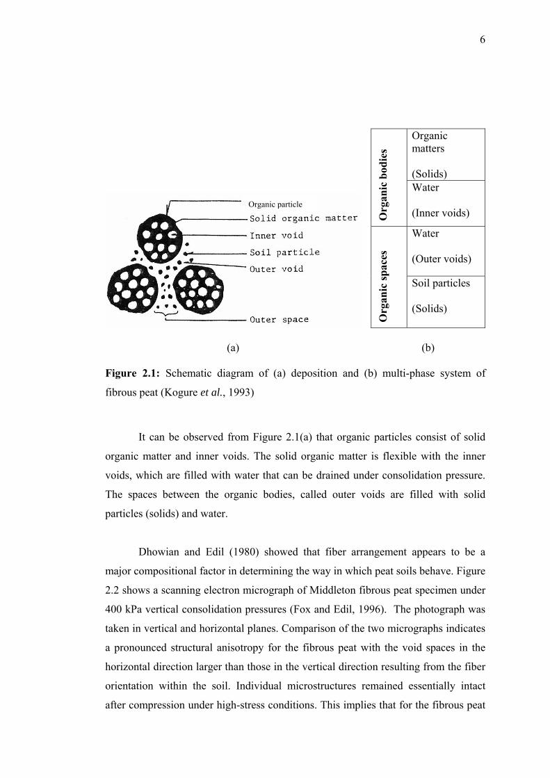
of mineral soils. Kogure et al. (1993) presented the idea of multi-phase system of

fibrous peat which consists of organic bodies and organic space. The organic body

consists of organic matter and water in inner voids, while the organic space consists

of water in outer voids and the soil particles. The solid organic matter can be drained

under consolidation pressure. The cross section of deposition and diagram of the

multi-phase system of fibrous peat are schematically shown in Figure 2.1(a) and (b).

6

(a)

Organic matters (Solids)

Org

anic

bod

ies

Water (Inner voids)

Water (Outer voids)

Org

anic

spac

es

Soil particles (Solids)

(b)

Organic particle

Figure 2.1: Schematic diagram of (a) deposition and (b) multi-phase system of

fibrous peat (Kogure et al., 1993)

It can be observed from Figure 2.1(a) that organic particles consist of solid

organic matter and inner voids. The solid organic matter is flexible with the inner

voids, which are filled with water that can be drained under consolidation pressure.

The spaces between the organic bodies, called outer voids are filled with solid

particles (solids) and water.

Dhowian and Edil (1980) showed that fiber arrangement appears to be a

major compositional factor in determining the way in which peat soils behave. Figure

2.2 shows a scanning electron micrograph of Middleton fibrous peat specimen under

400 kPa vertical consolidation pressures (Fox and Edil, 1996). The photograph was

taken in vertical and horizontal planes. Comparison of the two micrographs indicates

a pronounced structural anisotropy for the fibrous peat with the void spaces in the

horizontal direction larger than those in the vertical direction resulting from the fiber

orientation within the soil. Individual microstructures remained essentially intact

after compression under high-stress conditions. This implies that for the fibrous peat

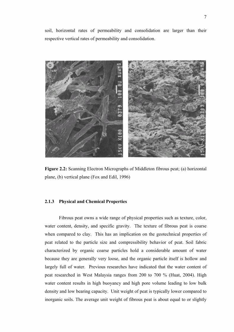
7

soil, horizontal rates of permeability and consolidation are larger than their

respective vertical rates of permeability and consolidation.

Figure 2.2: Scanning Electron Micrographs of Middleton fibrous peat; (a) horizontal

plane, (b) vertical plane (Fox and Edil, 1996)

2.1.3 Physical and Chemical Properties

Fibrous peat owns a wide range of physical properties such as texture, color,

water content, density, and specific gravity. The texture of fibrous peat is coarse

when compared to clay. This has an implication on the geotechnical properties of

peat related to the particle size and compressibility behavior of peat. Soil fabric

characterized by organic coarse particles hold a considerable amount of water

because they are generally very loose, and the organic particle itself is hollow and

largely full of water. Previous researches have indicated that the water content of

peat researched in West Malaysia ranges from 200 to 700 % (Huat, 2004). High

water content results in high buoyancy and high pore volume leading to low bulk

density and low bearing capacity. Unit weight of peat is typically lower compared to

inorganic soils. The average unit weight of fibrous peat is about equal to or slightly

8

higher than the unit weight of water. A range of 8.3–11.5 kN/m3 is common for unit

weight of fibrous peat in West Malaysia (Huat, 2004).

Specific gravity of fibrous peat soil ranges from 1.3 to 1.8 with an average of

1.5 (Ajlouni, 2000). The low specific gravity is due to low mineral content of the

soil. Natural void ratio of peat is generally higher than that of inorganic soils

indicating their higher capacity for compression. Natural void ratio of 5-15 is

common and a value as high as 25 have been reported for fibrous peat (Hanharan,

1954). Peat will shrink extensively when dried. The shrinkage could reach 50% of

the initial volume, but the dried peat will not swell up upon re-saturation because

dried peat cannot absorb water as much as initial condition; only 33% to 55% of the

water can be reabsorbed (Mokhtar, 1998).

Generally, peat soils are very acidic with low pH values, often lies between 4

and 7 (Lea, 1956). Peat existing in Peninsular Malaysia is known to have very low

pH values ranging from 3.0 to 4.5, and the acidity tends to decrease with depth

(Muttalib et.al., 1991). The submerged organic component of peat is not entirely

inert but undergoes very slow decomposition, accompanied by the production of

methane and less amount of nitrogen and carbon dioxide and hydrogen sulfide. Gas

content affects all physical properties measured and field performance that relates to

compression and water flow. A gas content of 5 to 10% of the total volume of the

soil is reported for peat and organic soils (Muskeg Engineering Handbook 1969).

2.1.4 Engineering Properties

Most fibrous peat is considered frictional or non-cohesive material (Adam,

1965) due to the fiber content, thus the shear strength of peat is determined based on

drained condition. The friction is mostly due to the fiber and the fiber is not always

solid because it is usually filled with water and gas, thus; the high friction angle does

not actually reflect the high shear strength of the soil. Shear box is the most common

test for determining the drained shear strength of fibrous peat, while triaxial test is

frequently used for laboratory evaluation of shear strength of peat under

consolidated-undrained condition (Noto, 1991).

9

Previous studies indicated that the effective internal friction φ' of peat is

generally higher than inorganic soil i.e: 50o for amorphous granular peat and in the

range of 53o–57o for fibrous peat (Edil and Dhowian, 1981). Landva (1983)

indicated the range of 27o–32o under a normal pressure of 30 to 50 kPa. The range

of internal friction angle of peat in West Malaysia is 3o–25o (Huat, 2004).

Considering the presence of peat soil is almost always below the groundwater

level, the determination of undrained shear strength is also important. This is usually

done in-situ because sampling of peat for laboratory evaluation of undrained shear

strength of fibrous peat is almost impossible. An undrained shear strength of peat soil

(Su) obtained by vane shear test was in range of 3 –15 kPa, which is much lower than

that of the mineral soils. A correction factor of 0.5 is suggested for the test results on

organic soil with a liquid limit of more than 200% (Hartlen and Wolsky, 1996).

Some approaches to in situ testing in peat deposits are: vane shear test, cone

penetration test, pressure-meter test, dilatometer test, plate load test and screw plate

load tests (Edil, 2001). Among them, the vane shear test is the most commonly used;

however, the interpretation of the test results must be handled with caution.

The compression behavior of fibrous peat is controlled by the fiber content.

Secondary compression is generally found as the more significant part of

compression because the time rate is much slower than the primary consolidation.

Determination of compressibility of fibrous peat is usually based on the standard

consolidation test.

Peat soils have a unit weight close to that of water; thus, the in-situ effective

stress (σ’o) is very small and sometimes cannot be detected from the results of

consolidation test. It is also very difficult to obtain the beginning of secondary

consolidation (tp) from consolidation curve because the preliminary consolidation

occurs rapidly. Natural void ratio (eo) is very high due to large pores, consequently;

the e-log p’ curves showed a steep slope indicating a high value of av and cc. The

compression index of peat soil ranges from 2 to 15. Furthermore, the secondary

consolidation may start before the dissipation of excess pore water pressure is

completed.

10

Compression of fibrous peat continues at a gradually decreasing rate under

constant effective stress, and this is termed as the secondary compression. The

secondary compression of peat is thought to be due to further decomposition of fiber

which is conveniently assumed to occur at a slower rate after the end of primary

consolidation. The rate of secondary compression is conveniently defined by the

slope (cα) of the final part of the void ratio versus log time curve. This estimate is

based on assumptions that cα is independent of time, thickness of compressible layer

and applied pressure. Ratio of cα/cc has been used widely to study the behavior of

peat. Mesri et al. (1994) reported a range between 0.05 and 0.07 for cα/cc.

2.1.5 Permeability

Permeability is one of the most important properties of peat because it

controls the rate of consolidation and increase in the shear strength of soil (Hobbs,

1986). Previous studies on physical and hydraulic properties of fibrous peat soil

indicate that the soil is averagely porous, and this certifies the fact that fibrous peat

soil has a medium degree of permeability. A range of the coefficient of permeability

of 10-5 to 10-8 m/s was obtained from previous studies (Colley, 1950 and Miyakawa,

1960).

Constant head permeability and Rowe consolidation cells have been used to

determine the vertical and horizontal coefficient of permeability of fibrous peat soil.

The permeability of peat depends on the void ratio, mineral content, degree of

decomposition of the peat, chemistry and the presence of gas. Mesri et al. (1997)

carried out permeability measurements during the secondary compression stage of

oedometer tests on Middleton peat. The study showed that a typical void ratio of 12,

Middleton peat is anisotropic with a value of kho/kvo = 10.

The change in permeability as a result of compression is drastic for fibrous

peat soils (Dhowian and Edil, 1980). Research on Portage fibrous peat shows the

soil initially has a relatively high permeability comparable to fine sand or silty sand,

11

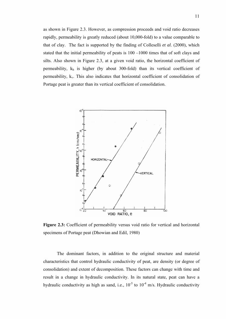
as shown in Figure 2.3. However, as compression proceeds and void ratio decreases

rapidly, permeability is greatly reduced (about 10,000-fold) to a value comparable to

that of clay. The fact is supported by the finding of Colleselli et al. (2000), which

stated that the initial permeability of peats is 100 –1000 times that of soft clays and

silts. Also shown in Figure 2.3, at a given void ratio, the horizontal coefficient of

permeability, kh is higher (by about 300-fold) than its vertical coefficient of

permeability, kv. This also indicates that horizontal coefficient of consolidation of

Portage peat is greater than its vertical coefficient of consolidation.

Figure 2.3: Coefficient of permeability versus void ratio for vertical and horizontal

specimens of Portage peat (Dhowian and Edil, 1980)

The dominant factors, in addition to the original structure and material

characteristics that control hydraulic conductivity of peat, are density (or degree of

consolidation) and extent of decomposition. These factors can change with time and

result in a change in hydraulic conductivity. In its natural state, peat can have a

hydraulic conductivity as high as sand, i.e., 10-5 to 10-4 m/s. Hydraulic conductivity

12

decreases markedly under load down to the level of silt or clay hydraulic

conductivity i.e., 10-8 to 10-9 m/s or even lower (Hillis and Brawner, 1961; Dhowian

and Edil, 1980; Lea and Brawner, 1963). According to Edil (2003), the rate of

decrease of hydraulic conductivity with decreasing void ratio is usually higher than

that in clays. The large decrease in hydraulic conductivity under continuous

compression implies that large strain theory of consolidation may be appropriate for

high water content fibrous peat (Lan, 1992).

2.2 Soil Compressibility

In general, the compressibility of a soil consists of three stages, namely initial

compression, primary consolidation and secondary compression. While initial

compression occurs instantaneously after the application of load, the primary and

secondary compressions are time dependent. The initial compression is due partly to

the compression of small pockets of gas within the pore spaces, and partly to the

elastic compression of soil grains. Primary consolidation is due to dissipation of

excess pore water pressure caused by an increase in effective stress whereas

secondary compression takes place under constant effective stress after the

completion of dissipation of excess pore water pressure.

The time required for the water to dissipate from the soil depends on the

permeability of the soil itself. In granular soil, the process is rapid and hardly

noticeable due to its high permeability. On the other hand, the consolidation process

may take years in clay soil. For peat, the primary consolidation occurs rapidly due to

high initial permeability and secondary compression takes a significant part of

compression.

2.2.1 Primary Consolidation

One-dimensional theory of consolidation developed by Terzaghi in 1925

carries an assumption that primary consolidation is due to dissipation of excess pore

13

water pressure caused by an increase in effective stress whereas secondary

compression takes place under constant effective stress after the completion of the

dissipation of excess pore water pressure. Other important assumptions attached to

the Terzaghi consolidation theory are that the flow is one-dimensional and the rate of

consolidation or permeability is constant throughout the consolidation process.

Consolidation characteristics of soil can be represented by consolidation

parameters such as coefficient of axial compressibility av, coefficient of volume

compressibility mv, compression index cc, and recompression index cr. Another

important characteristic of soil compressibility is the pre-consolidation pressure (σc’).

The soil that has been loaded and unloaded will be less compressible when it is

reloaded again, thus; settlement will not usually be great when the applied load

remains below the pre consolidation pressure. These parameters can be estimated

from a curve relating void ratio (e) at the end of each increment period against the

corresponding load increment in linear scale (Figure 2.4) or log scale (Figure 2.5).

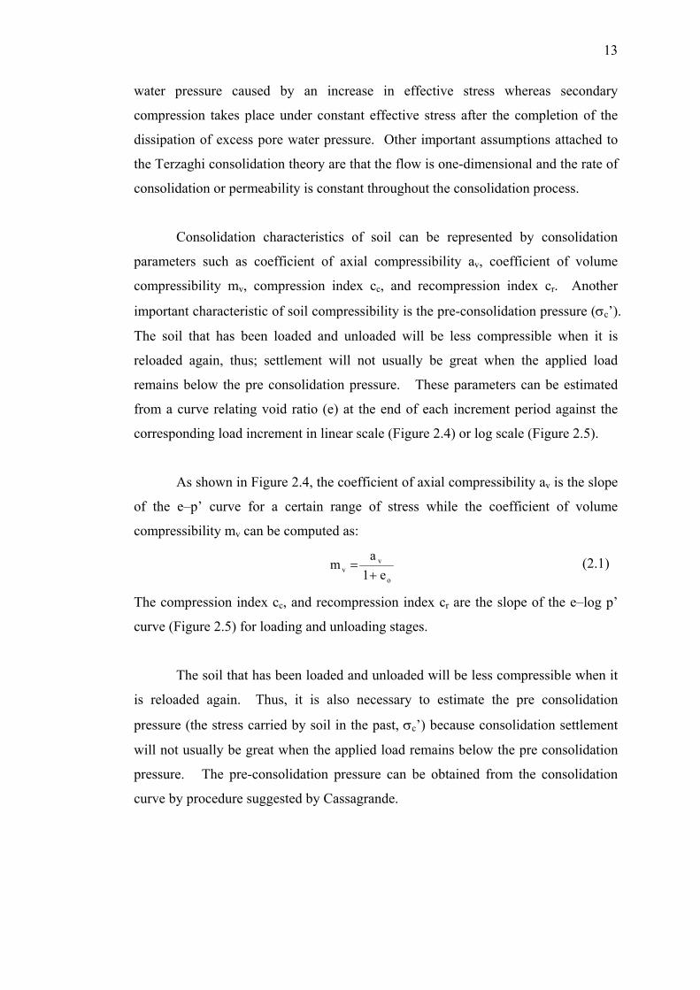
As shown in Figure 2.4, the coefficient of axial compressibility av is the slope

of the e–p’ curve for a certain range of stress while the coefficient of volume

compressibility mv can be computed as:

o

vv e1

am

+= (2.1)

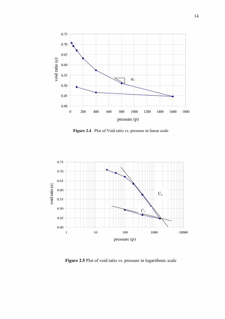
The compression index cc, and recompression index cr are the slope of the e–log p’

curve (Figure 2.5) for loading and unloading stages.

The soil that has been loaded and unloaded will be less compressible when it

is reloaded again. Thus, it is also necessary to estimate the pre consolidation

pressure (the stress carried by soil in the past, σc’) because consolidation settlement

will not usually be great when the applied load remains below the pre consolidation

pressure. The pre-consolidation pressure can be obtained from the consolidation

curve by procedure suggested by Cassagrande.

14

0.40

0.45

0.50

0.55

0.60

0.65

0.70

0.75

0 200 400 600 800 1000 1200 1400 1600 1800

pressure (p)

void

ratio

(e)

av

Figure 2.4 Plot of Void ratio vs. pressure in linear scale

0.40

0.45

0.50

0.55

0.60

0.65

0.70

0.75

1 10 100 1000 10000

pressure (p)

void

ratio

(e)

Cr

Cc

Figure 2.5 Plot of void ratio vs. pressure in logarithmic scale

15

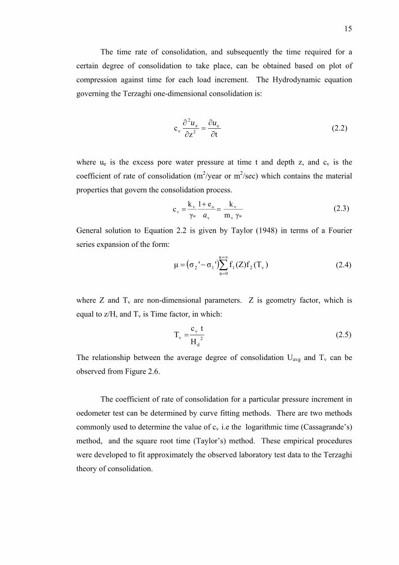
The time rate of consolidation, and subsequently the time required for a

certain degree of consolidation to take place, can be obtained based on plot of

compression against time for each load increment. The Hydrodynamic equation

governing the Terzaghi one-dimensional consolidation is:

tzc e

2

2

∂∂

=∂∂ uu e

v (2.2)

where ue is the excess pore water pressure at time t and depth z, and cv is the

coefficient of rate of consolidation (m2/year or m2/sec) which contains the material

properties that govern the consolidation process.

wv

v

v

o

w

vv γm

ke1γk

c =+

=a

(2.3)

General solution to Equation 2.2 is given by Taylor (1948) in terms of a Fourier

series expansion of the form:

( )∑∞=

=

−=n

0nv2112 )(T(Z)ff'σ'σµ (2.4)

where Z and Tv are non-dimensional parameters. Z is geometry factor, which is

equal to z/H, and Tv is Time factor, in which:

2d

vv H

tcT = (2.5)

The relationship between the average degree of consolidation Uavg and Tv can be

observed from Figure 2.6.

The coefficient of rate of consolidation for a particular pressure increment in

oedometer test can be determined by curve fitting methods. There are two methods

commonly used to determine the value of cv i.e the logarithmic time (Cassagrande’s)

method, and the square root time (Taylor’s) method. These empirical procedures

were developed to fit approximately the observed laboratory test data to the Terzaghi

theory of consolidation.

16

Figure 2.6 Consolidation curve for two-way vertical drainage (Head, 1982)

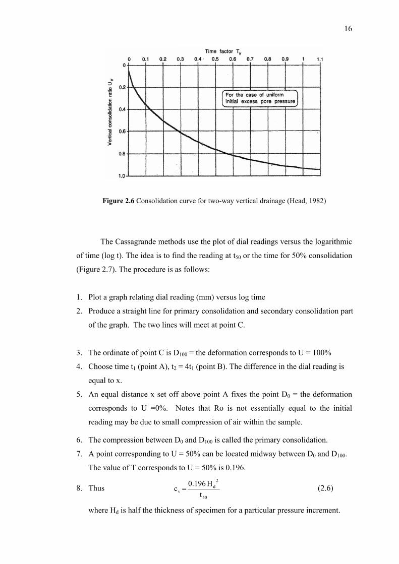
The Cassagrande methods use the plot of dial readings versus the logarithmic

of time (log t). The idea is to find the reading at t50 or the time for 50% consolidation

(Figure 2.7). The procedure is as follows:

1. Plot a graph relating dial reading (mm) versus log time

2. Produce a straight line for primary consolidation and secondary consolidation part

of the graph. The two lines will meet at point C.

3. The ordinate of point C is D100 = the deformation corresponds to U = 100%

4. Choose time t1 (point A), t2 = 4t1 (point B). The difference in the dial reading is

equal to x.

5. An equal distance x set off above point A fixes the point D0 = the deformation

corresponds to U =0%. Notes that Ro is not essentially equal to the initial

reading may be due to small compression of air within the sample.

6. The compression between D0 and D100 is called the primary consolidation.

7. A point corresponding to U = 50% can be located midway between D0 and D100.

The value of T corresponds to U = 50% is 0.196.

8. Thus 50

2d

v tH0.196c = (2.6)

where Hd is half the thickness of specimen for a particular pressure increment.

17

3.84.04.24.44.64.85.05.25.45.65.86.06.26.46.66.8

1 10 100 1000 10000

time (minutes)

dial

read

ing

(D)

Figure 2.7 Determination of cv by Cassagrande method

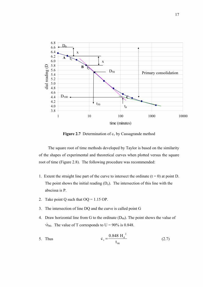
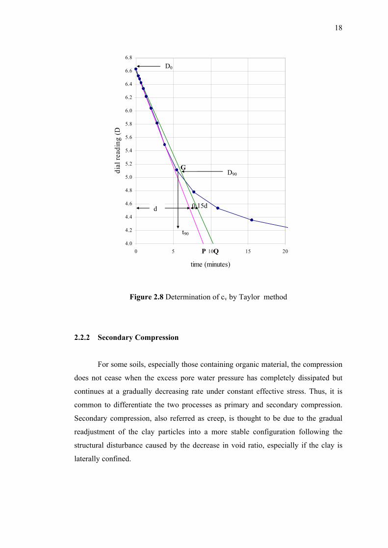
The square root of time methods developed by Taylor is based on the similarity

of the shapes of experimental and theoretical curves when plotted versus the square

root of time (Figure 2.8). The following procedure was recommended:

1. Extent the straight line part of the curve to intersect the ordinate (t = 0) at point D.

The point shows the initial reading (Do). The intersection of this line with the

abscissa is P.

2. Take point Q such that OQ = 1.15 OP.

3. The intersection of line DQ and the curve is called point G

4. Draw horizontal line from G to the ordinate (D90). The point shows the value of

√t90. The value of T corresponds to U = 90% is 0.848.

5. Thus 90

2d

v tH0.848c = (2.7)

tp

D100 C

t1

t2

x

D0

x A

B D50 Primary consolidation

t50

18

4.0

4.2

4.4

4.6

4.8

5.0

5.2

5.4

5.6

5.8

6.0

6.2

6.4

6.6

6.8

0 5

D0

Figure 2.8 Determination of cv by Taylor method

2.2.2 Secondary Compression

For some soils, especially those containing organic material, the compression

does not cease when the excess pore water pressure has completely dissipated but

continues at a gradually decreasing rate under constant effective stress. Thus, it is

common to differentiate the two processes as primary and secondary compression.

Secondary compression, also referred as creep, is thought to be due to the gradual

readjustment of the clay particles into a more stable configuration following the

structural disturbance caused by the decrease in void ratio, especially if the clay is

laterally confined.

10P 15 20

time (minutes)

dial

read

ing

(D

Q

G D90

0.15d d

t90

19

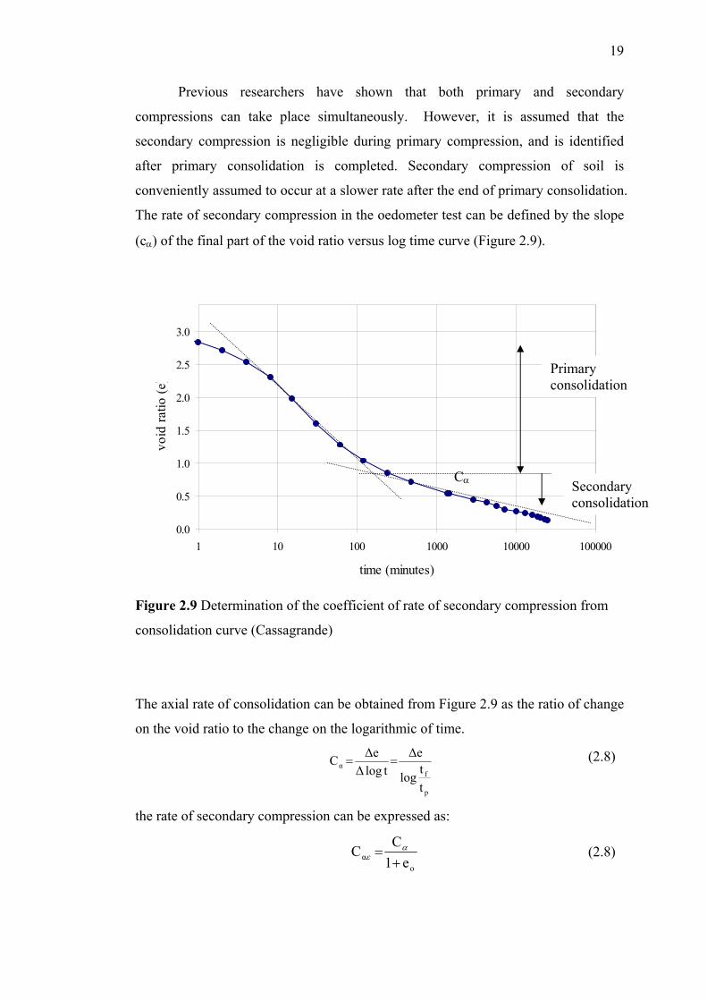
Previous researchers have shown that both primary and secondary

compressions can take place simultaneously. However, it is assumed that the

secondary compression is negligible during primary compression, and is identified

after primary consolidation is completed. Secondary compression of soil is

conveniently assumed to occur at a slower rate after the end of primary consolidation.

The rate of secondary compression in the oedometer test can be defined by the slope

(cα) of the final part of the void ratio versus log time curve (Figure 2.9).

0.0

0.5

1.0

1.5

2.0

2.5

3.0

1 10 100 1000 10000 100000

time (minutes)

void

ratio

(e)

Figure 2.9 Determination of the coefficient of rate of secondary compression from

consolidation curve (Cassagrande)

Secondary consolidation

Primary consolidation

Cα

The axial rate of consolidation can be obtained from Figure 2.9 as the ratio of change

on the void ratio to the change on the logarithmic of time.

p

fα

ttlog

∆etlog∆

∆eC == (2.8)

the rate of secondary compression can be expressed as:

oα e1

CC

+= α

ε (2.8)

20

in which ∆e is the change of void ratio from tp to tf. tp denotes the time of the

completion of primary consolidation, while tf is the time for which the secondary

consolidation settlement is required. The void ratio at time tp is denoted as eo. This

estimate is based on assumptions that cα is independent of time, thickness of

compressible layer and applied pressure. Research showed that the ratio of cα/cc is

almost constant and varies from 0.025 to 0.06 for inorganic soil, while a slightly high

range was obtained for organic soils and peats (Holtz and Kovacs, 1981).

2.3 Large Strain Consolidation Test

The compressibility characteristics of a soil are usually determined from

consolidation tests. General laboratory tests for measurement of compression and

consolidation characteristics of a soil are: Oedometer consolidation test, Constant

Rate of Strain (CRS) test, and Rowe Cell test. The procedures for these tests are

fully described in BS 1377-6 and Head (1982, 1986).

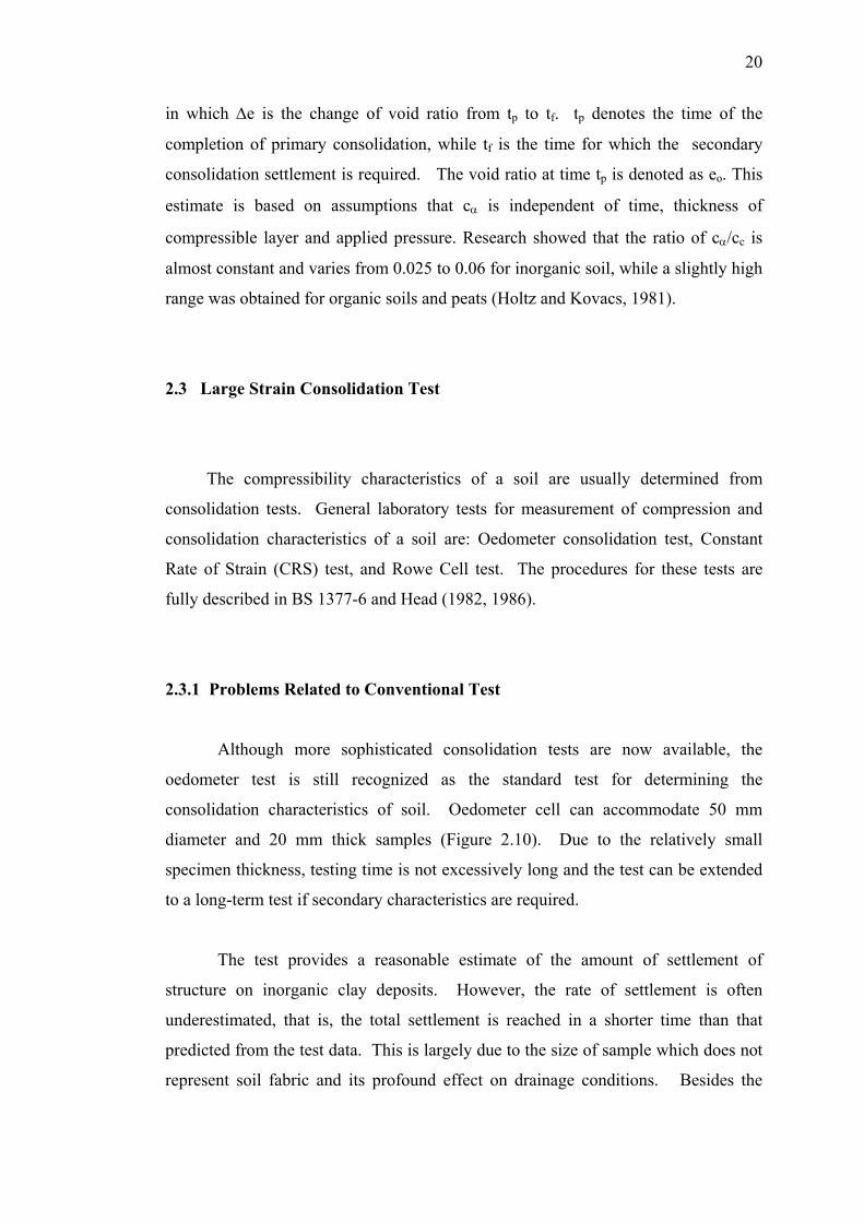
2.3.1 Problems Related to Conventional Test

Although more sophisticated consolidation tests are now available, the

oedometer test is still recognized as the standard test for determining the

consolidation characteristics of soil. Oedometer cell can accommodate 50 mm

diameter and 20 mm thick samples (Figure 2.10). Due to the relatively small

specimen thickness, testing time is not excessively long and the test can be extended

to a long-term test if secondary characteristics are required.

The test provides a reasonable estimate of the amount of settlement of

structure on inorganic clay deposits. However, the rate of settlement is often

underestimated, that is, the total settlement is reached in a shorter time than that

predicted from the test data. This is largely due to the size of sample which does not

represent soil fabric and its profound effect on drainage conditions. Besides the

21

natural condition of the sample, sampling disturbance will have a more pronounced

effect on the results of the test done on small samples. Furthermore, the boundary

effect from the ring enhances the friction of the sample. Friction reduces the stress

acted on the soil during loading and reduces swelling during unloading.

Soil samplePorous stones

ho ∆h

Consolidation ring

Consolidation ring

Applied pressure

Figure 2.10 Schematic diagram of Oedometer Cell

For standard test, the samples were subjected to consolidation pressures with

load increment ratio of one. The load is applied through a mechanical lever arm

system, thus: measurement can be easily affected by sudden shock. Excessive

disturbance affects the e - log p’ plot and tends to obscure the effect of stress history;

gives low values of pre-consolidation pressure and over-consolidation ratio, and

gives high coefficient of volume compressibility at low stresses. Excessive

disturbance also reduces the effect of secondary compression which is a very

important characteristic of fibrous peat.

The other limitation of oedometer test is that there is no means of measuring

excess pore-water pressures, the dissipation of which control the consolidation

process. Therefore the estimation of compressibility is based solely on the change of

height of the specimen.

22

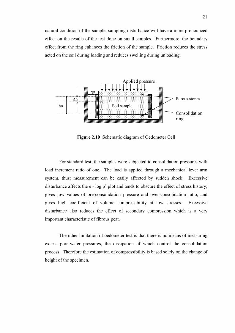
2.3.2 Large Strain Test (Rowe Cell)

Rowe consolidation cell (Figure 2.11) was introduced by Rowe and Barden in

1966 to overcome the disadvantages of the conventional oedometer apparatus when

performing consolidation tests on non-uniform deposits such as fibrous peat. Rowe

cell has many advantages over the conventional Oedometer consolidation apparatus.

The main features responsible for these improvements are the hydraulic loading

system; the control facilities and ability to measure pore water pressure, and the

capability of testing samples of large diameter.

Figure 2.11 Schematic diagram of Rowe Consolidation cell

Through hydraulic loading system, the sample is less susceptible to vibration

effects and higher pressures can be applied easily due to large sample size. The

hydraulic loading system enables samples of large diameter up to 254 mm diameter

to be tested for practical purposes and allows for large settlement deformations. The

use of large samples enables the effect of the soil fabric (laminations, fissures,

bedding planes) to be taken into account in the consolidation process, thereby

enabling a realistic estimate of the rate of consolidation to be made. Large samples

have been found to give higher and more reliable values of cv, especially under low

stresses, than conventional oedometer test samples (Head, 1986). Better agreement

has been reported between predicted and observed rates of settlement, as well as their

magnitude, may be partly due to the relatively smaller effect of structural viscosity

23

and fabric in larger samples. Tests on high quality large diameter samples minimize

the effect of sample disturbance and therefore provide more reliable data for

settlement analysis than conventional one-dimensional oedometer tests on small

samples.

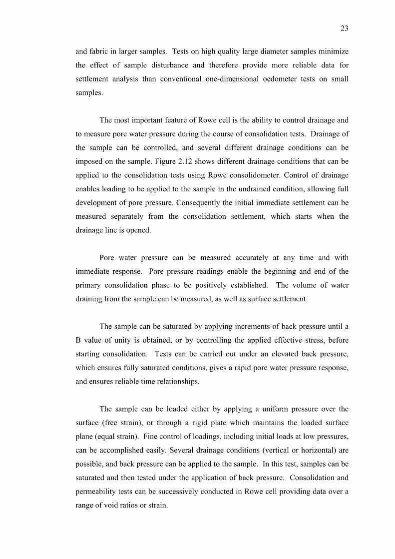
The most important feature of Rowe cell is the ability to control drainage and

to measure pore water pressure during the course of consolidation tests. Drainage of

the sample can be controlled, and several different drainage conditions can be

imposed on the sample. Figure 2.12 shows different drainage conditions that can be

applied to the consolidation tests using Rowe consolidometer. Control of drainage

enables loading to be applied to the sample in the undrained condition, allowing full

development of pore pressure. Consequently the initial immediate settlement can be

measured separately from the consolidation settlement, which starts when the

drainage line is opened.

Pore water pressure can be measured accurately at any time and with

immediate response. Pore pressure readings enable the beginning and end of the

primary consolidation phase to be positively established. The volume of water

draining from the sample can be measured, as well as surface settlement.

The sample can be saturated by applying increments of back pressure until a

B value of unity is obtained, or by controlling the applied effective stress, before

starting consolidation. Tests can be carried out under an elevated back pressure,

which ensures fully saturated conditions, gives a rapid pore water pressure response,

and ensures reliable time relationships.

The sample can be loaded either by applying a uniform pressure over the

surface (free strain), or through a rigid plate which maintains the loaded surface

plane (equal strain). Fine control of loadings, including initial loads at low pressures,

can be accomplished easily. Several drainage conditions (vertical or horizontal) are

possible, and back pressure can be applied to the sample. In this test, samples can be

saturated and then tested under the application of back pressure. Consolidation and

permeability tests can be successively conducted in Rowe cell providing data over a

range of void ratios or strain.

24

Figure 2.12 : Drainage and loading conditions for consolidations tests in Rowe cell: (a),(c), (e), (g) with ‘free strain’ loading, (b), (d), (f), (h) with ‘equal strain’ loading (Head, 1986)

25

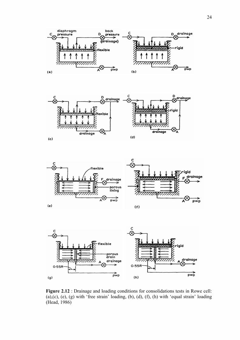
2.4 Analysis of Time-Compression curve

Figure 2.13 shows three types of time-compression curve derived from

laboratory consolidation test on different types of soil (Leonards and Girault, 1961).

Type I curve is defined by Terzaghi’s theory with S-shaped curve. The separation of

primary and secondary compression from Type I curve is relatively easy because it

follows that the secondary compression occurs at a slower rate after the dissipation of

pore water pressure. Identification of the beginning of secondary consolidation (tp)

and the rate of secondary compression (cα) for type I curve can be estimated based

on Cassagrande method as explained in Section 2.2.2.

Figure 2.13 Types of time-compression curve derived from consolidation test

(Leonards and Girault, 1961)

Researches showed that the time compression curves derived from results of

one-dimensional consolidation test on fibrous peat soil do not follow the type I curve.

They resemble the type II curve in which the primary consolidation is very rapid and

secondary compression does not vary linearly with logarithmic of time and tertiary

compression is actually observed after secondary compression. Therefore the

quantification of secondary compression based on conventional (Cassagrande)

method frequently under-estimate the settlement. Dhowian and Edil (1980) extended

the Cassagrande method to include the nonlinearity of secondary compression of

26

fibrous peat by a coefficient of secondary compression, cα1, and coefficient of

tertiary compression, cα2 (Figure 2.13). In this case, time of secondary compression

(ts) should be identified in addition to the time for primary consolidation (tp). The

term ‘tertiary strain’ is introduced as a soil strain to designate the increasing

coefficient of secondary compression with time.

It is evident that the conventional method assumes that the secondary

compression begins at the completion of pore-water pressure (tp = t100), and this can

be evaluated from time–settlement curve. The methods also assumed that the

secondary compression occurs at a slower rate then the primary consolidation, thus tp

is obtained at the inflexion point in the curve. The method cannot evaluate

secondary compression of soils exhibiting Type III curve (Figure 2.13) because the

curve does not show an inflection point.

Previous researcher (Robinson, 1997) have pointed out that the full

dissipation of pore water pressure cannot be predicted based on settlement curve

because based on his findings on consolidation test with measurement of pore water

pressure, the pore water pressure dissipation is completed earlier than the time

predicted from the inflection point of the settlement curve. Further analysis by the

same researcher (Robinson, 2003) revealed that the secondary compression actually

starts during the dissipation of excess pore-water pressure from the soil. This

observation was based on Terzaghi’s one dimensional consolidation theory, whereby

the relationship between dissipation of excess pore water pressure and compression

during primary consolidation can be represented by a straight line while the actual

curve derived from laboratory consolidation test on peat soil was not actually

follows a straight line. Thus, the settlement was actually due to combination of pore

water pressure dissipation on primary consolidation and secondary compression.

Robinson (2003) suggested a method for separating the primary consolidation

and secondary compression that occur during the consolidation process. The method

was developed based on time–compression and the time–pore water pressure curves

(Figure 2.14).

27

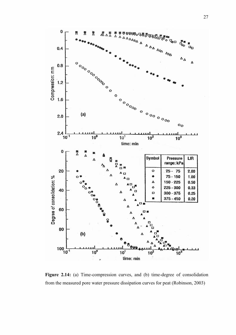
Figure 2.14: (a) Time-compression curves, and (b) time-degree of consolidation

from the measured pore water pressure dissipation curves for peat (Robinson, 2003)

28

It can be observed that the dissipation of pore water pressure dissipation

(Figure 2.14(b)) is actually completed earlier than predicted by the settlement curve

(Figure 2.14(a)). Some settlement curves do not exhibit the inflection point, that the

end of primary consolidation cannot be predicted based on Cassagrande method.

According to Robinson (2003), the data from Figure 2.14(a) and 2.14(b) can be

plotted as degree of consolidation measured from the dissipation of excess pore

water pressure versus total compression of the soil in Figure 2.15(a)-(f).

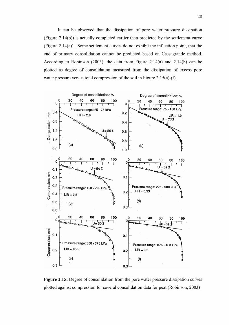
Figure 2.15: Degree of consolidation from the pore water pressure dissipation curves

plotted against compression for several consolidation data for peat (Robinson, 2003)

29

Figure 2.15 (a) to (f) show similar trend in which the curve deviate from a

straight line at a certain degree of consolidation. The point where the curve diverges

from linearity is identified as the beginning of secondary compression. The

compression corresponding to the point where the straight line meets the U = 100%

axis is the total primary consolidation settlement (δp), while the compression below

the extrapolated line is the secondary compression (δs). Thus, using this procedure, it

is possible to separate the primary consolidation settlement and secondary

compression from time-compression data obtained from the laboratory one-

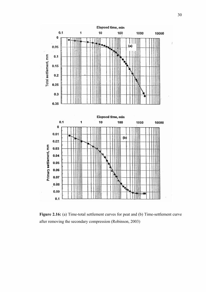
dimensional consolidation test. Figure 2.16 (a) and (b) show the total and primary

consolidation settlement after the removal of secondary compression respectively. A

clear S or Type I curve is obtained which is the shape expected if only the primary

consolidation is considered (Figure 2.16 (b)).

The secondary compression-time relationship is commonly represented by a

logarithmic function. Instead of using the consolidation curve derived directly from

test results, the evaluation of the coefficient of consolidation of peat soil should be

based on the primary consolidation versus logarithmic of time curve (Figure 2.16(b)).

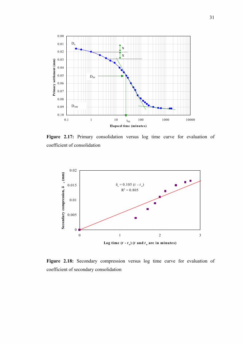
This figure is redrawn in Figure 2.17 for the purpose of describing the evaluating the

coefficient of consolidation. The starting and ending ordinates of the primary

consolidation curve are regarded as the beginning and ending of primary

consolidation (D0 and D100) of soil respectively. The corresponding times are denoted

by t0 and t100 respectively. The time for 50% primary consolidation can be obtained

from D50 which is the midpoint between d0 and d100. For one-dimensional two-way

vertical drainage, coefficient of consolidation (cv) can be calculated by Equation 2.6.

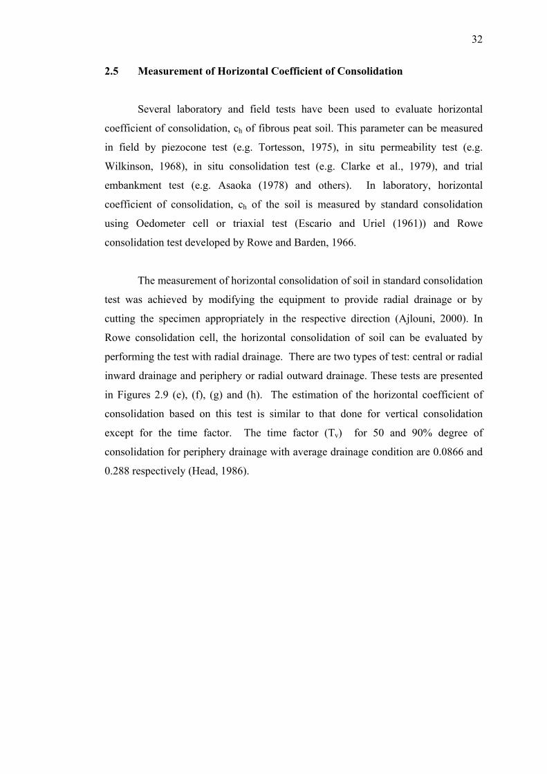
For Robinson’s method, as long as the secondary compression varies linearly

with logarithmic of time, the time-secondary compression relationship is

satisfactorily represented by the coefficient of secondary compression. The plot can

be obtained by subtracting the primary consolidation from total settlement. Note that

zero secondary settlement was obtained for t equal to to, where to is the beginning of

secondary consolidation. Figure 2.18 shows the plot of the secondary compression

(δs) against their corresponding time (t–to). The coefficient of secondary

compression of soil (cα) is the slope of the line shown in Figure 2.18.

30

Figure 2.16: (a) Time-total settlement curves for peat and (b) Time-settlement curve

after removing the secondary compression (Robinson, 2003)

31

0.00

0.01

0.02

0.03

0.04

0.05

0.06

0.07

0.08

0.09

0.100.1 1 10

Elapse

Prim

ary

sett

lem

ent (

mm

)

x

D50

D100

Do

Figure 2.17: Primary consolidatio

coefficient of consolidation

δs

0

0.005

0.01

0.015

0.02

0

Log time

Seco

ndar

y co

mpr

essio

n, δ

s (m

m)

Figure 2.18: Secondary compressi

coefficient of secondary consolidatio

x

100 1000 10000

d time (minutes)t50

n versus log time curve for evaluation of

= 0.105 (t - t o)R2 = 0.805

1 2

(t - t o) (t and t o are in minutes)

3

on versus log time curve for evaluation of

n

32

2.5 Measurement of Horizontal Coefficient of Consolidation

Several laboratory and field tests have been used to evaluate horizontal

coefficient of consolidation, ch of fibrous peat soil. This parameter can be measured

in field by piezocone test (e.g. Tortesson, 1975), in situ permeability test (e.g.

Wilkinson, 1968), in situ consolidation test (e.g. Clarke et al., 1979), and trial

embankment test (e.g. Asaoka (1978) and others). In laboratory, horizontal

coefficient of consolidation, ch of the soil is measured by standard consolidation

using Oedometer cell or triaxial test (Escario and Uriel (1961)) and Rowe

consolidation test developed by Rowe and Barden, 1966.

The measurement of horizontal consolidation of soil in standard consolidation

test was achieved by modifying the equipment to provide radial drainage or by

cutting the specimen appropriately in the respective direction (Ajlouni, 2000). In

Rowe consolidation cell, the horizontal consolidation of soil can be evaluated by

performing the test with radial drainage. There are two types of test: central or radial

inward drainage and periphery or radial outward drainage. These tests are presented

in Figures 2.9 (e), (f), (g) and (h). The estimation of the horizontal coefficient of

consolidation based on this test is similar to that done for vertical consolidation

except for the time factor. The time factor (Tv) for 50 and 90% degree of

consolidation for periphery drainage with average drainage condition are 0.0866 and

0.288 respectively (Head, 1986).

33

CHAPTER 3

METHODOLOGY

3.1 Introduction

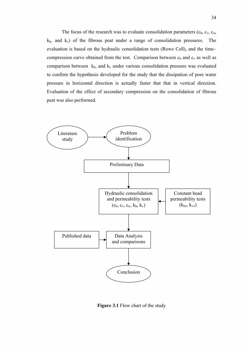
The study was an experimental research, which concentrate on the evaluation

of coefficient of rate of horizontal consolidation of fibrous peat. The methodology of

the research is summarized in the flowchart shown in Figure 3.1. Literature study

was made to provide rationale of the research and to gather sufficient information on

the consolidation behavior of fibrous peat. The samples of fibrous peat were

obtained from Kampung Bahru, Pontian, Johor from depth of 1 to 2 m below the

ground surface, thus, the sample is considered as surface peat. The sampling method

is described in report for UTM fundamental research vot 75137 (2006). The organic

and fiber content of the peat as well as the degree of humification obtained from

previous research have shown that the soil can be classified as fibrous peat.

The scanning Electron Micrograph was performed to evaluate the structural

arrangement of the peat. Engineering characteristics evaluated in this research

include consolidation and permeability test. Preliminary evaluation of the

consolidation characteristics of the soil is based on the standard consolidation test.

Constant-head permeability tests were carried out to determine initial hydraulic

conductivity of the peat. All laboratory test procedures are based on the manual of

soil laboratory testing (Head, 1981, 1982, 1986) in accordance with the British

Standards (BS) and American Standard Testing Methods (ASTM).

34

The focus of the research was to evaluate consolidation parameters (ch, cv, cα,

kh, and kv) of the fibrous peat under a range of consolidation pressures. The

evaluation is based on the hydraulic consolidation tests (Rowe Cell), and the time–

compression curve obtained from the test. Comparison between ch and cv as well as

comparison between kh, and kv under various consolidation pressure was evaluated

to confirm the hypothesis developed for the study that the dissipation of pore water

pressure in horizontal direction is actually faster that that in vertical direction.

Evaluation of the effect of secondary compression on the consolidation of fibrous

peat was also performed.

Literature study

Hydraulic consolidation and permeability tests

(ch, cv, cα, kh, kv)

Data Analysis and comparisons

Published data

Preliminary Data

Problem identification

Conclusion

Constant head permeability tests

(kho, kvo)

Figure 3.1 Flow chart of the study

35

3.2 Preliminary data

Most of the preliminary data for the research such as physical and chemical

characteristics and classification of the peat under study were acquired from report

for fundamental research vot 75137 (2006). Standard consolidation test data useful

for establishing the rate of consolidation pressure to be used in the large strain

consolidation test was also obtained from the report.

Considering the published range of initial permeability of fibrous peat,

constant head permeability test was adopted in this study to determine the initial

permeability of the soil in horizontal and vertical directions. The constant head

permeability test was done on sample obtained vertically and horizontally using

piston sampler. The tests are done following standard procedures of ASTM D2434.

Scanning Electron Micrograph were done in this research to determine the

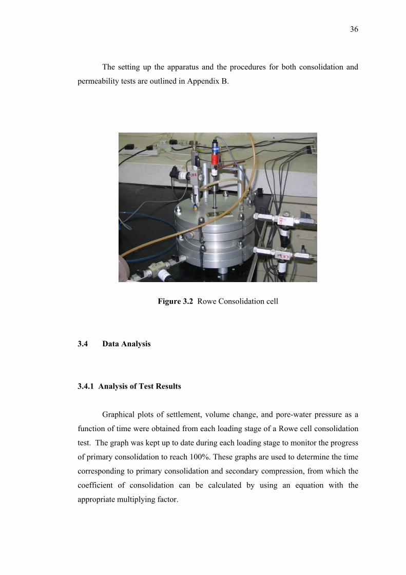
structural arrangement of the soil as the basis for the analysis on the horizontal

coefficient of consolidation and the effect of secondary compression on the

consolidation of the peat. The test follows the standard procedure outlined in ASTM

F 1392-93.

3.3 Large Strain Consolidation Test

Evaluation of the coefficient of consolidation in vertical and horizontal

direction was performed on large strain consolidation tests using Rowe consolidation

cell (Figure 3.2) with internal diameter of 150 mm and height of 50 mm. The

vertical consolidation was tested under two-way vertical drainage, while the

horizontal consolidation was evaluated by horizontal drainage to periphery. Under

both conditions, the soil samples were subjected to hydraulic consolidation pressures

of 25, 50, 100, and 200 kPa.

The effect of consolidation pressure on fabric arrangement and therefore the

permeability of the peat were studied by carrying out permeability test on Rowe cell

under consolidation pressure of 100 and 200 kPa for vertical and horizontal drainage.

36

The setting up the apparatus and the procedures for both consolidation and

permeability tests are outlined in Appendix B.

Figure 3.2 Rowe Consolidation cell

3.4 Data Analysis

3.4.1 Analysis of Test Results

Graphical plots of settlement, volume change, and pore-water pressure as a

function of time were obtained from each loading stage of a Rowe cell consolidation

test. The graph was kept up to date during each loading stage to monitor the progress

of primary consolidation to reach 100%. These graphs are used to determine the time

corresponding to primary consolidation and secondary compression, from which the

coefficient of consolidation can be calculated by using an equation with the

appropriate multiplying factor.

37

Wherever possible, it is better to use the pore pressure dissipation graph

rather than the settlement or volume change curve because the end points (0% and

100% dissipation) are both clearly defined and t50 or t90 can be read directly from the

graph. The t50 point is preferable because the mid portion of the curve best fit to the

theoretical curve. Settlement and volume-change measurements are governed by the

deformation of the sample as a whole, and analysis is dependent on an overall

‘average’ behavior.

Besides the time compression curve, a graph relating the void ratio at the end

of each loading stage with the effective pressure on a linear or logarithmic scale was

plotted for a complete set of consolidation test data. The e–p’ curve is used to obtain

coefficient of axial compressibility av and thus the coefficient of volume

compressibility mv, while the e–log p’ is used to obtain compression and

recompression indexes, cc and cr respectively. Pre-consolidation pressure can also be

obtained if possible. These data are required for evaluation of the magnitude of

primary settlement and to obtain the ratio of cα/cc for calculation of secondary

compression.

3.4.2 Analysis of Time-Compression Curve

The time-compression curves derived from test results were analyzed based

on Cassagrande and Robinson methods. The secondary compression index as well as

the beginning and end of secondary compression are among the parameters required

for the analysis of secondary compression. Furthermore the settlement and the

coefficient of rate of consolidation cv was calculated based on the curve.

Cassagrande method requires a compression–log time curve to evaluate the

parameters. The detailed procedure for analysis of time–compression curve by

Cassagrande method is outlined in Sections 2.2.1 and 2.2.2. Besides the

compression–log time curve, the pore-water pressure–log time curve is required for

evaluation of the parameters by Robinson’s method. These plots are used to develop

compression–degree of consolidation graph as the basis for determination of

38

settlement and cv. The procedures for evaluation of settlement and coefficient of

consolidation cv by Robinson’s method is outlined in Section 2.4.

3.4.3 Analysis of output

As pointed out in the beginning, the output of the study is presented in terms

of coefficient of consolidation and permeability in horizontal and vertical directions

ch, cv, kh, kv, as well as the effect of secondary compression cα, These values were

evaluated and compared. The ratios of ch/cv and kh/kv can be used for analysis on the

effect of fabric on the properties. The ratio of cα/cc can be used as a basis for

evaluation of secondary compression of the peat. These results were compared to the

published data on similar type of soil.

39

CHAPTER 4

RESULTS AND DISCUSSION

4.1 Introduction

The discussion in this chapter will follow the stated objectives of the study

mentioned in Chapter 1. Section 4.2 presents the results of the laboratory test on

the soil identification and consolidation characteristics based on the standard

Oedometer test obtained from previous research (UTM Fundamental vot 75137).

Section 4.3 deals with the study on the fiber orientation of the soil sample which

is very useful on the analysis of horizontal coefficient of consolidation.

The main focus of the study is to determine the horizontal coefficient of

consolidation on Rowe consolidation test, and the results are compared with the

vertical coefficient of consolidation. The results of the test and the analysis of the

compression curves obtained from the tests are given in Section 4.4. Effect of

secondary compression on the consolidation behavior in both directions is

discussed in Section 4.5.

Fiber orientation influences the permeability of soil and application of

pressure affects the fiber orientation, thus; permeability characteristics are

evaluated in the study. Section 4.6 presents the analysis on the initial

40

permeability obtained from constant head permeability test, permeability obtained

from consolidation test and the permeability calculated from the coefficient of

consolidation. Comparisons on the horizontal and vertical permeability are also

subject of analysis.

4.2 Soil identification

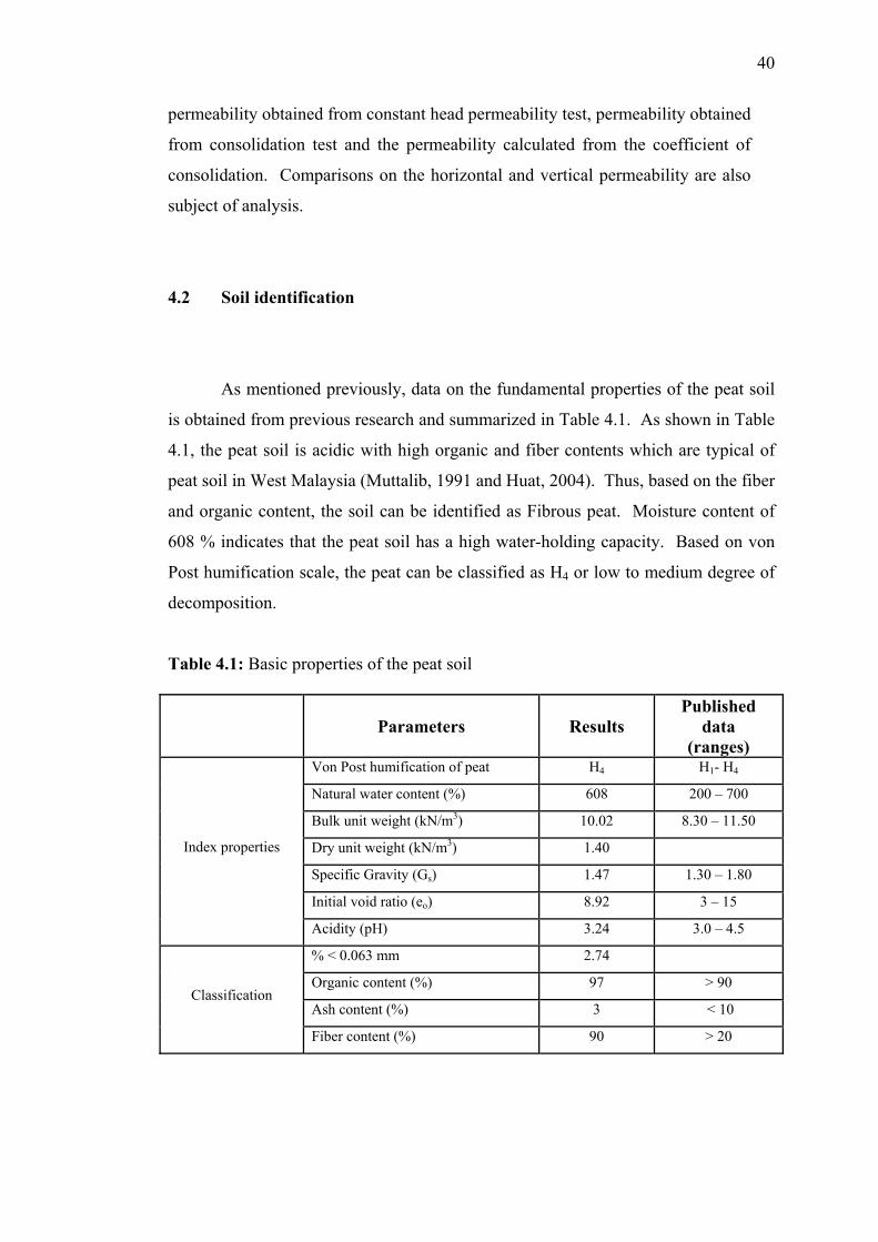
As mentioned previously, data on the fundamental properties of the peat soil

is obtained from previous research and summarized in Table 4.1. As shown in Table

4.1, the peat soil is acidic with high organic and fiber contents which are typical of

peat soil in West Malaysia (Muttalib, 1991 and Huat, 2004). Thus, based on the fiber

and organic content, the soil can be identified as Fibrous peat. Moisture content of

608 % indicates that the peat soil has a high water-holding capacity. Based on von

Post humification scale, the peat can be classified as H4 or low to medium degree of

decomposition.

Table 4.1: Basic properties of the peat soil

Parameters

Results

Published data

(ranges) Von Post humification of peat H4 H1- H4

Natural water content (%) 608 200 – 700

Bulk unit weight (kN/m3) 10.02 8.30 – 11.50

Dry unit weight (kN/m3) 1.40

Specific Gravity (Gs) 1.47 1.30 – 1.80

Initial void ratio (eo) 8.92 3 – 15

Index properties

Acidity (pH) 3.24 3.0 – 4.5

% < 0.063 mm 2.74

Organic content (%) 97 > 90

Ash content (%) 3 < 10 Classification

Fiber content (%) 90 > 20

41

Standard Oedometer test was conducted on 12 samples. Each of the samples

has a thickness of 20.13 mm, a diameter of 50.23 mm, and was subjected to

consolidation pressures of 12.5 kPa, 25 kPa, 50 kPa, 100 kPa, 200 kPa, and 400 kPa.

The results indicate that primary consolidation and secondary compression

characteristics of the soil can be easily identified from consolidation curves.

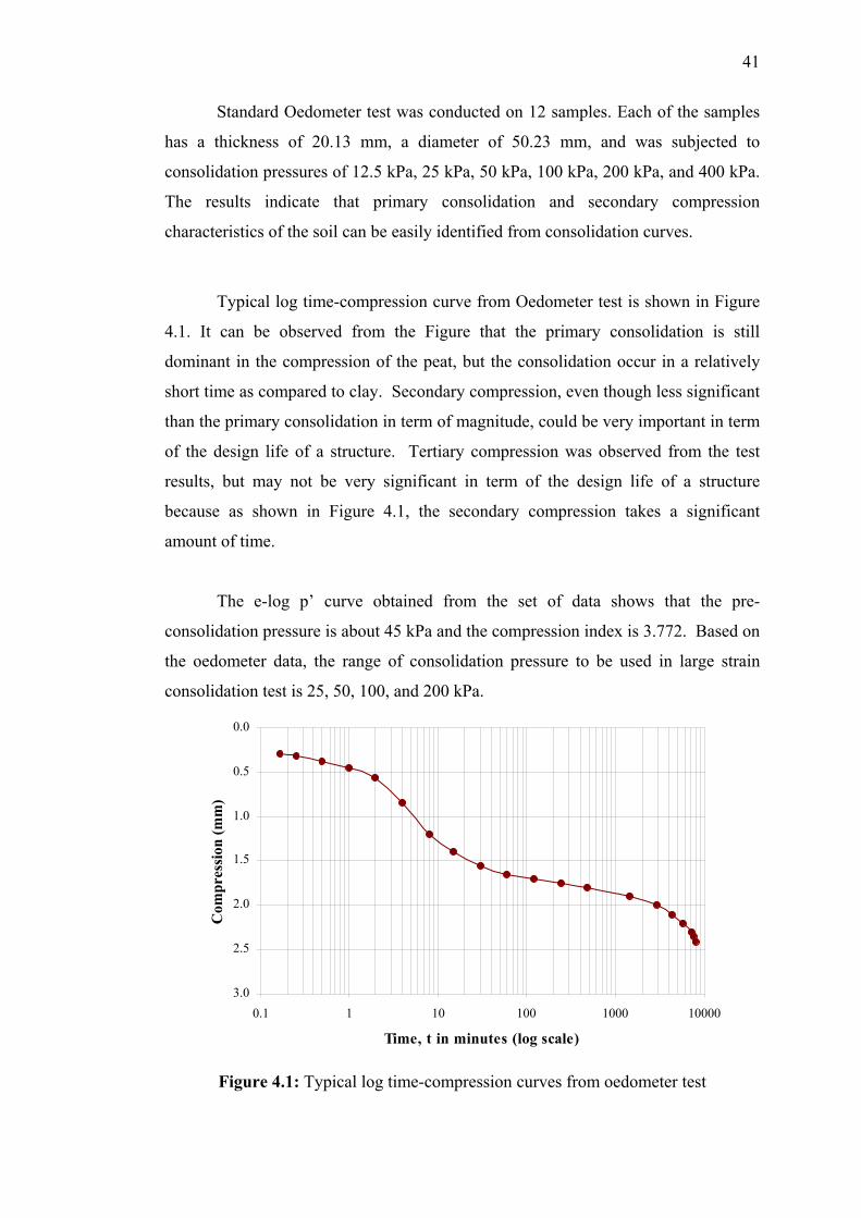
Typical log time-compression curve from Oedometer test is shown in Figure

4.1. It can be observed from the Figure that the primary consolidation is still

dominant in the compression of the peat, but the consolidation occur in a relatively

short time as compared to clay. Secondary compression, even though less significant

than the primary consolidation in term of magnitude, could be very important in term

of the design life of a structure. Tertiary compression was observed from the test

results, but may not be very significant in term of the design life of a structure

because as shown in Figure 4.1, the secondary compression takes a significant

amount of time.

The e-log p’ curve obtained from the set of data shows that the pre-

consolidation pressure is about 45 kPa and the compression index is 3.772. Based on

the oedometer data, the range of consolidation pressure to be used in large strain

consolidation test is 25, 50, 100, and 200 kPa.

0.0

0.5

1.0

1.5

2.0

2.5

3.00.1 1 10 100 1000 10000

Time, t in minutes (log scale)

Com

pres

sion

(mm

)

Figure 4.1: Typical log time-compression curves from oedometer test

42

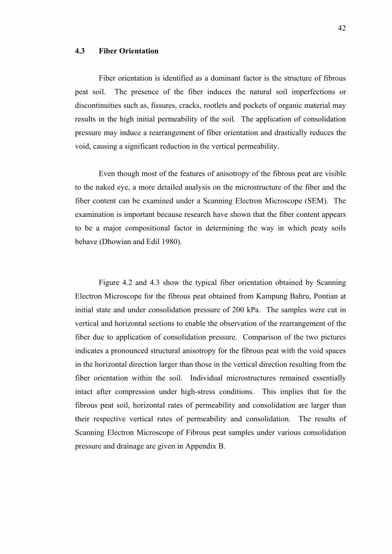
4.3 Fiber Orientation

Fiber orientation is identified as a dominant factor is the structure of fibrous

peat soil. The presence of the fiber induces the natural soil imperfections or

discontinuities such as, fissures, cracks, rootlets and pockets of organic material may

results in the high initial permeability of the soil. The application of consolidation

pressure may induce a rearrangement of fiber orientation and drastically reduces the

void, causing a significant reduction in the vertical permeability.

Even though most of the features of anisotropy of the fibrous peat are visible

to the naked eye, a more detailed analysis on the microstructure of the fiber and the

fiber content can be examined under a Scanning Electron Microscope (SEM). The

examination is important because research have shown that the fiber content appears

to be a major compositional factor in determining the way in which peaty soils

behave (Dhowian and Edil 1980).

Figure 4.2 and 4.3 show the typical fiber orientation obtained by Scanning

Electron Microscope for the fibrous peat obtained from Kampung Bahru, Pontian at

initial state and under consolidation pressure of 200 kPa. The samples were cut in

vertical and horizontal sections to enable the observation of the rearrangement of the

fiber due to application of consolidation pressure. Comparison of the two pictures

indicates a pronounced structural anisotropy for the fibrous peat with the void spaces

in the horizontal direction larger than those in the vertical direction resulting from the

fiber orientation within the soil. Individual microstructures remained essentially

intact after compression under high-stress conditions. This implies that for the

fibrous peat soil, horizontal rates of permeability and consolidation are larger than

their respective vertical rates of permeability and consolidation. The results of

Scanning Electron Microscope of Fibrous peat samples under various consolidation

pressure and drainage are given in Appendix B.

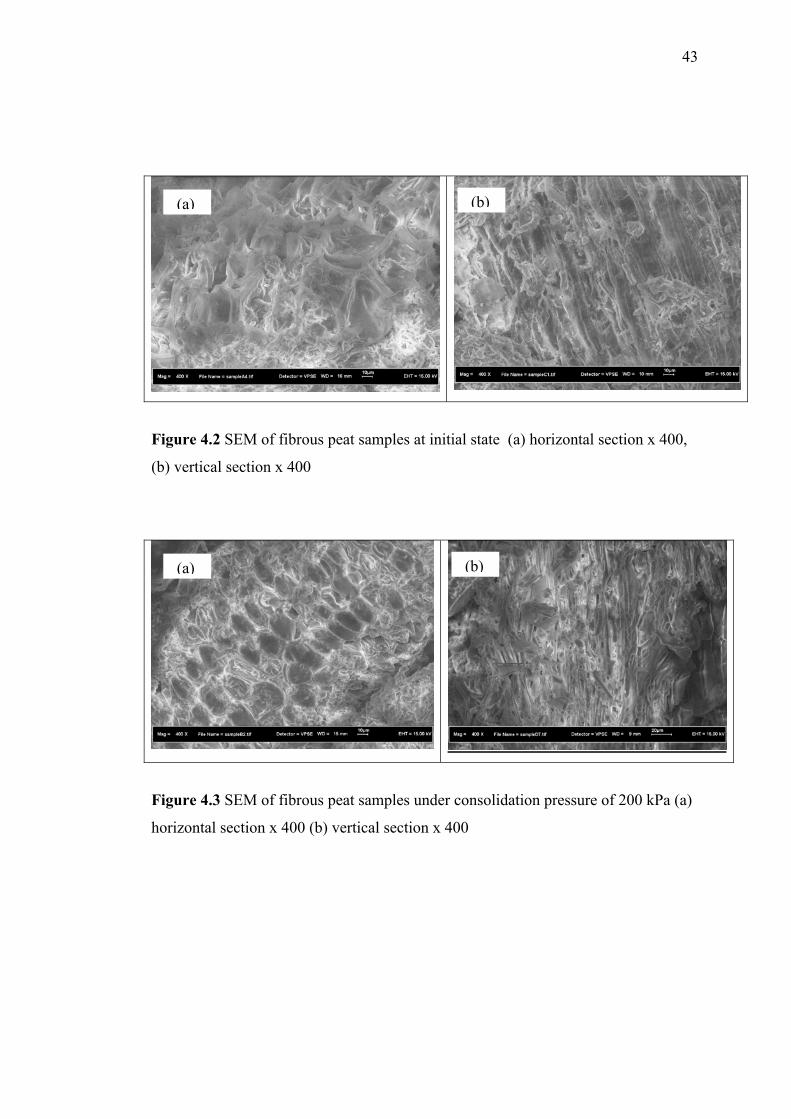
43

(b) (a)

Figure 4.2 SEM of fibrous peat samples at initial state (a) horizontal section x 400,

(b) vertical section x 400

(b) (a)

Figure 4.3 SEM of fibrous peat samples under consolidation pressure of 200 kPa (a)

horizontal section x 400 (b) vertical section x 400

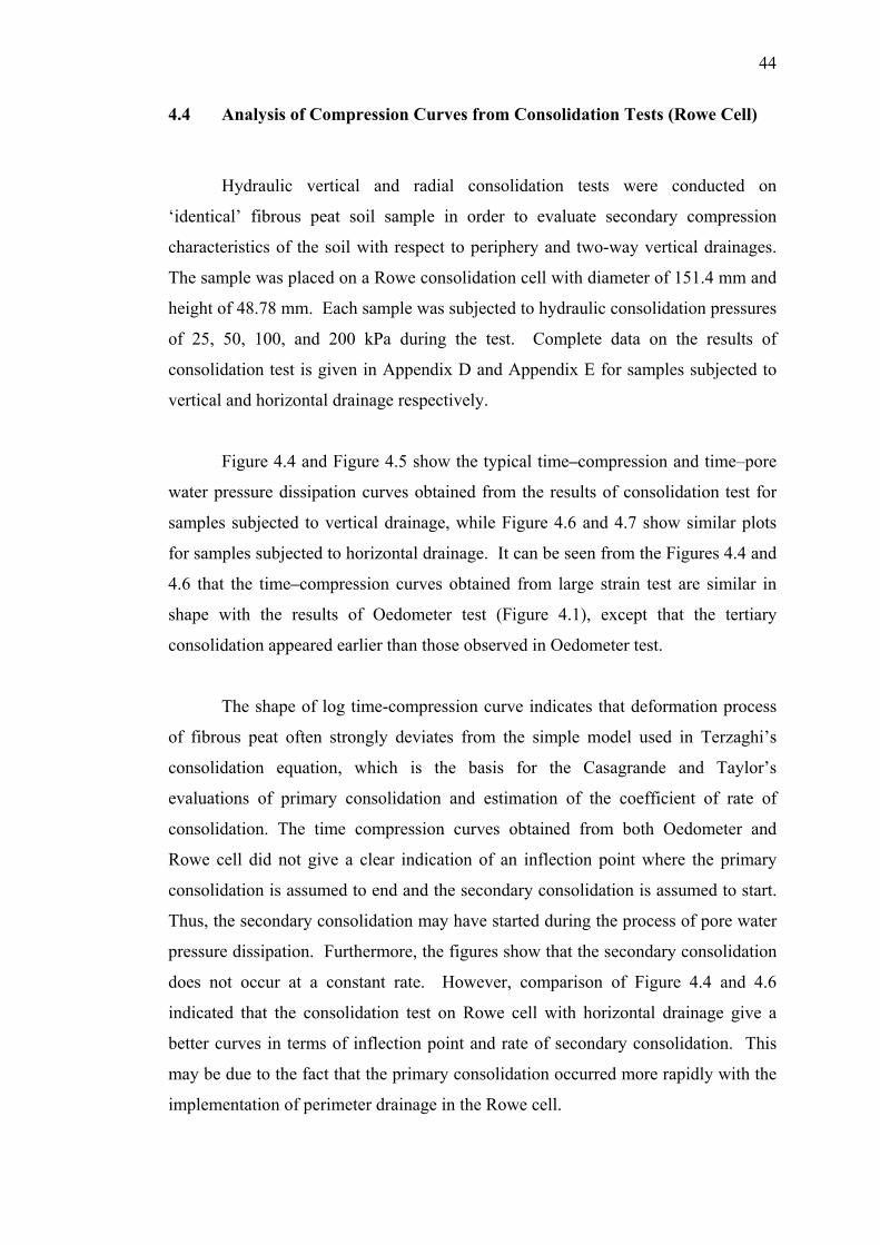
44

4.4 Analysis of Compression Curves from Consolidation Tests (Rowe Cell)

Hydraulic vertical and radial consolidation tests were conducted on

‘identical’ fibrous peat soil sample in order to evaluate secondary compression

characteristics of the soil with respect to periphery and two-way vertical drainages.

The sample was placed on a Rowe consolidation cell with diameter of 151.4 mm and

height of 48.78 mm. Each sample was subjected to hydraulic consolidation pressures

of 25, 50, 100, and 200 kPa during the test. Complete data on the results of

consolidation test is given in Appendix D and Appendix E for samples subjected to

vertical and horizontal drainage respectively.

Figure 4.4 and Figure 4.5 show the typical time–compression and time–pore

water pressure dissipation curves obtained from the results of consolidation test for

samples subjected to vertical drainage, while Figure 4.6 and 4.7 show similar plots

for samples subjected to horizontal drainage. It can be seen from the Figures 4.4 and

4.6 that the time–compression curves obtained from large strain test are similar in

shape with the results of Oedometer test (Figure 4.1), except that the tertiary

consolidation appeared earlier than those observed in Oedometer test.

The shape of log time-compression curve indicates that deformation process

of fibrous peat often strongly deviates from the simple model used in Terzaghi’s

consolidation equation, which is the basis for the Casagrande and Taylor’s

evaluations of primary consolidation and estimation of the coefficient of rate of

consolidation. The time compression curves obtained from both Oedometer and

Rowe cell did not give a clear indication of an inflection point where the primary

consolidation is assumed to end and the secondary consolidation is assumed to start.

Thus, the secondary consolidation may have started during the process of pore water

pressure dissipation. Furthermore, the figures show that the secondary consolidation

does not occur at a constant rate. However, comparison of Figure 4.4 and 4.6

indicated that the consolidation test on Rowe cell with horizontal drainage give a

better curves in terms of inflection point and rate of secondary consolidation. This

may be due to the fact that the primary consolidation occurred more rapidly with the

implementation of perimeter drainage in the Rowe cell.

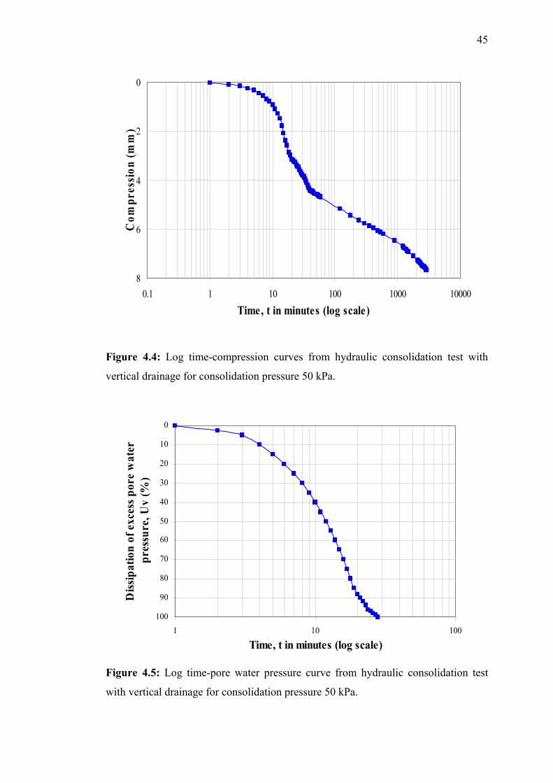
45

0

2

4

6

80.1 1 10 100 1000 10000

Time, t in minutes (log scale)

Com

pres

sion

(mm

)

Figure 4.4: Log time-compression curves from hydraulic consolidation test with

vertical drainage for consolidation pressure 50 kPa.

0

10

20

30

40

50

60

70

80

90

1001 10 100

Time, t in minutes (log scale)

Diss

ipat

ion

of e

xces

s por

e w

ater

pr

essu

re, U

v (%

)

Figure 4.5: Log time-pore water pressure curve from hydraulic consolidation test

with vertical drainage for consolidation pressure 50 kPa.

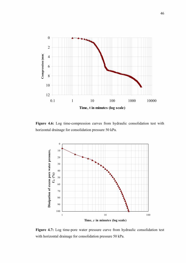
46

0

2

4

6

8

10

120.1 1 10 100 1000 10000

Time, t in minutes (log scale)

Com

pres

sion

(mm

)

Figure 4.6: Log time-compression curves from hydraulic consolidation test with

horizontal drainage for consolidation pressure 50 kPa.

0

10

20

30

40

50

60

70

80

90

1001 10 100

Time, t in minutes (log scale)

Diss

ipat

ion

of e

xces

s por

e w

ater

pre

ssur

e,U

h (%

)

Figure 4.7: Log time-pore water pressure curve from hydraulic consolidation test

with horizontal drainage for consolidation pressure 50 kPa.

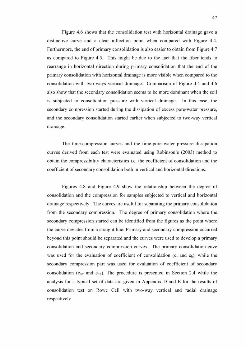
47

Figure 4.6 shows that the consolidation test with horizontal drainage gave a

distinctive curve and a clear inflection point when compared with Figure 4.4.

Furthermore, the end of primary consolidation is also easier to obtain from Figure 4.7

as compared to Figure 4.5. This might be due to the fact that the fiber tends to

rearrange in horizontal direction during primary consolidation that the end of the

primary consolidation with horizontal drainage is more visible when compared to the

consolidation with two ways vertical drainage. Comparison of Figure 4.4 and 4.6

also show that the secondary consolidation seems to be more dominant when the soil

is subjected to consolidation pressure with vertical drainage. In this case, the

secondary compression started during the dissipation of excess pore-water pressure,

and the secondary consolidation started earlier when subjected to two-way vertical

drainage.

The time-compression curves and the time-pore water pressure dissipation

curves derived from each test were evaluated using Robinson’s (2003) method to

obtain the compressibility characteristics i.e. the coefficient of consolidation and the

coefficient of secondary consolidation both in vertical and horizontal directions.

Figures 4.8 and Figure 4.9 show the relationship between the degree of

consolidation and the compression for samples subjected to vertical and horizontal

drainage respectively. The curves are useful for separating the primary consolidation

from the secondary compression. The degree of primary consolidation where the

secondary compression started can be identified from the figures as the point where

the curve deviates from a straight line. Primary and secondary compression occurred

beyond this point should be separated and the curves were used to develop a primary

consolidation and secondary compression curves. The primary consolidation cuve

was used for the evaluation of coefficient of consolidation (cv and ch), while the

secondary compression part was used for evaluation of coefficient of secondary

consolidation (cαv and cαh). The procedure is presented in Section 2.4 while the

analysis for a typical set of data are given in Appendix D and E for the results of

consolidation test on Rowe Cell with two-way vertical and radial drainage

respectively.

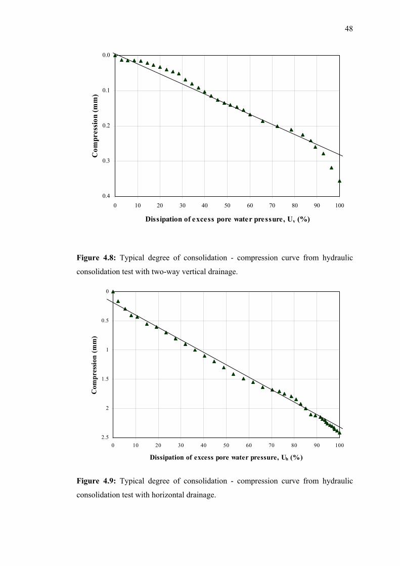
48

0.0

0.1

0.2

0.3

0.40 10 20 30 40 50 60 70 80 90 100

Dissipation of excess pore water pressure, Uv (%)

Com

pres

sion

(mm

)

Figure 4.8: Typical degree of consolidation - compression curve from hydraulic

consolidation test with two-way vertical drainage.

0

0.5

1

1.5

2

2.50 10 20 30 40 50 60 70 80 90 10

Dissipation of excess pore water pressure, Uh (%)

Com

pres

sion

(mm

)

0

Figure 4.9: Typical degree of consolidation - compression curve from hydraulic

consolidation test with horizontal drainage.

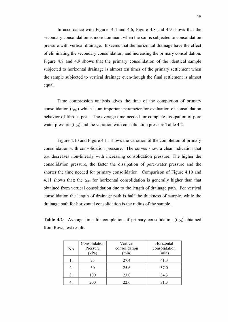
49

In accordance with Figures 4.4 and 4.6, Figure 4.8 and 4.9 shows that the

secondary consolidation is more dominant when the soil is subjected to consolidation

pressure with vertical drainage. It seems that the horizontal drainage have the effect

of eliminating the secondary consolidation, and increasing the primary consolidation.

Figure 4.8 and 4.9 shows that the primary consolidation of the identical sample

subjected to horizontal drainage is almost ten times of the primary settlement when

the sample subjected to vertical drainage even-though the final settlement is almost

equal.

Time compression analysis gives the time of the completion of primary

consolidation (t100) which is an important parameter for evaluation of consolidation

behavior of fibrous peat. The average time needed for complete dissipation of pore

water pressure (t100) and the variation with consolidation pressure Table 4.2.

Figure 4.10 and Figure 4.11 shows the variation of the completion of primary

consolidation with consolidation pressure. The curves show a clear indication that

t100 decreases non-linearly with increasing consolidation pressure. The higher the

consolidation pressure, the faster the dissipation of pore-water pressure and the

shorter the time needed for primary consolidation. Comparison of Figure 4.10 and

4.11 shows that: the t100 for horizontal consolidation is generally higher than that

obtained from vertical consolidation due to the length of drainage path. For vertical

consolidation the length of drainage path is half the thickness of sample, while the

drainage path for horizontal consolidation is the radius of the sample.

Table 4.2: Average time for completion of primary consolidation (t100) obtained

from Rowe test results

No

ConsolidationPressure

(kPa)

Vertical consolidation

(min)

Horizontal consolidation

(min)

1. 25 27.4 41.3

2. 50 25.6 37.0

3. 100 23.0 34.3

4. 200 22.6 31.3

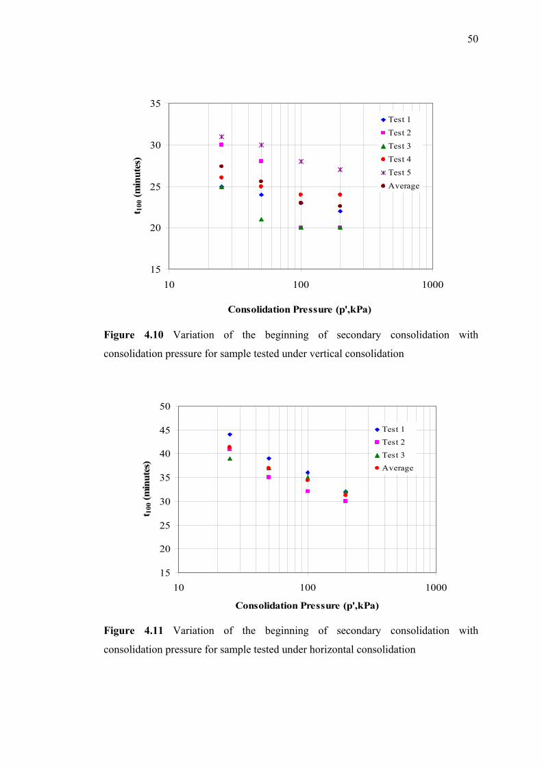
50

15

20

25

30

35

10 100 1000

Consolidation Pressure (p',kPa)

t 100

(min

utes

)

Test 1Test 2Test 3Test 4Test 5Average

Figure 4.10 Variation of the beginning of secondary consolidation with

consolidation pressure for sample tested under vertical consolidation

15

20

25

30

35

40

45

50

10 100 1000

Consolidation Pressure (p',kPa)

t 100

(min

utes

)

Test 1Test 2Test 3Average

Figure 4.11 Variation of the beginning of secondary consolidation with

consolidation pressure for sample tested under horizontal consolidation

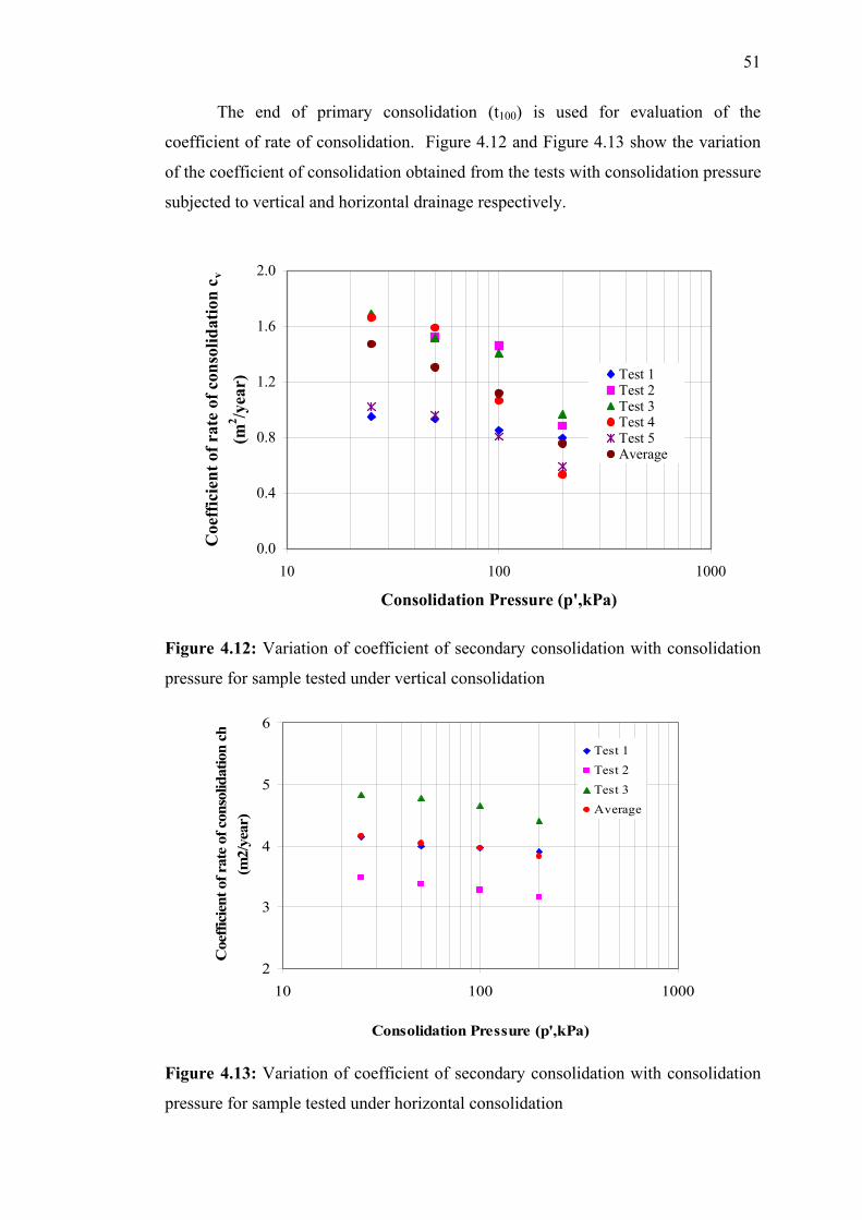
51

The end of primary consolidation (t100) is used for evaluation of the

coefficient of rate of consolidation. Figure 4.12 and Figure 4.13 show the variation

of the coefficient of consolidation obtained from the tests with consolidation pressure

subjected to vertical and horizontal drainage respectively.

0.0

0.4

0.8

1.2

1.6

2.0

10 100 1000

Consolidation Pressure (p',kPa)

Coe

ffic

ient

of r

ate

of c

onso

lidat

ion

c v(m

2 /yea

r) Test 1Test 2Test 3Test 4Test 5Average

Figure 4.12: Variation of coefficient of secondary consolidation with consolidation

pressure for sample tested under vertical consolidation

2

3

4

5

6

10 100 1000

Consolidation Pressure (p',kPa)

Coe

ffici

ent o

f rat

e of

con

solid

atio

n ch

(m2/

year

)

Test 1Test 2Test 3Average

Figure 4.13: Variation of coefficient of secondary consolidation with consolidation

pressure for sample tested under horizontal consolidation

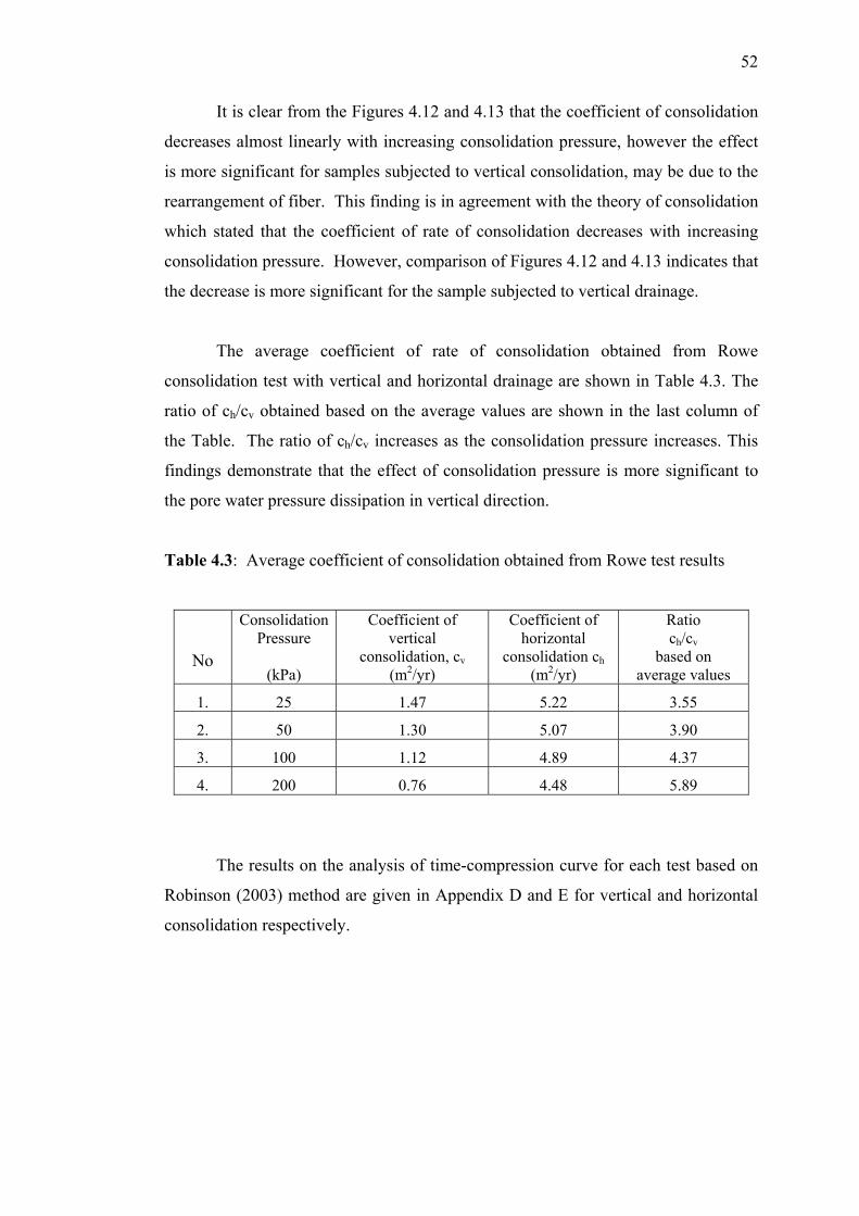
52

It is clear from the Figures 4.12 and 4.13 that the coefficient of consolidation

decreases almost linearly with increasing consolidation pressure, however the effect

is more significant for samples subjected to vertical consolidation, may be due to the

rearrangement of fiber. This finding is in agreement with the theory of consolidation

which stated that the coefficient of rate of consolidation decreases with increasing

consolidation pressure. However, comparison of Figures 4.12 and 4.13 indicates that

the decrease is more significant for the sample subjected to vertical drainage.

The average coefficient of rate of consolidation obtained from Rowe

consolidation test with vertical and horizontal drainage are shown in Table 4.3. The

ratio of ch/cv obtained based on the average values are shown in the last column of

the Table. The ratio of ch/cv increases as the consolidation pressure increases. This

findings demonstrate that the effect of consolidation pressure is more significant to

the pore water pressure dissipation in vertical direction.

Table 4.3: Average coefficient of consolidation obtained from Rowe test results

No

Consolidation Pressure

(kPa)

Coefficient of vertical

consolidation, cv (m2/yr)

Coefficient of horizontal

consolidation ch (m2/yr)

Ratio ch/cv

based on average values

1. 25 1.47 5.22 3.55

2. 50 1.30 5.07 3.90

3. 100 1.12 4.89 4.37

4. 200 0.76 4.48 5.89

The results on the analysis of time-compression curve for each test based on

Robinson (2003) method are given in Appendix D and E for vertical and horizontal

consolidation respectively.

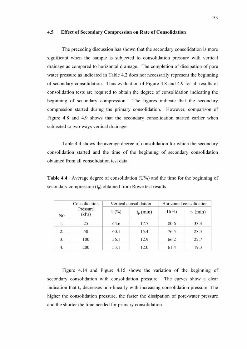
53

4.5 Effect of Secondary Compression on Rate of Consolidation

The preceding discussion has shown that the secondary consolidation is more

significant when the sample is subjected to consolidation pressure with vertical

drainage as compared to horizontal drainage. The completion of dissipation of pore

water pressure as indicated in Table 4.2 does not necessarily represent the beginning

of secondary consolidation. Thus evaluation of Figure 4.8 and 4.9 for all results of

consolidation tests are required to obtain the degree of consolidation indicating the

beginning of secondary compression. The figures indicate that the secondary

compression started during the primary consolidation. However, comparison of

Figure 4.8 and 4.9 shows that the secondary consolidation started earlier when

subjected to two-ways vertical drainage.

Table 4.4 shows the average degree of consolidation for which the secondary

consolidation started and the time of the beginning of secondary consolidation

obtained from all consolidation test data.

Table 4.4: Average degree of consolidation (U%) and the time for the beginning of

secondary compression (tp) obtained from Rowe test results

Vertical consolidation Horizontal consolidation

No

Consolidation Pressure

(kPa) U(%) tp (min) U(%) tp (min)

1. 25 64.6 17.7 80.6 33.3

2. 50 60.1 15.4 76.5 28.3

3. 100 56.1 12.9 66.2 22.7

4. 200 53.1 12.0 61.4 19.3

Figure 4.14 and Figure 4.15 shows the variation of the beginning of

secondary consolidation with consolidation pressure. The curves show a clear

indication that tp decreases non-linearly with increasing consolidation pressure. The

higher the consolidation pressure, the faster the dissipation of pore-water pressure

and the shorter the time needed for primary consolidation.

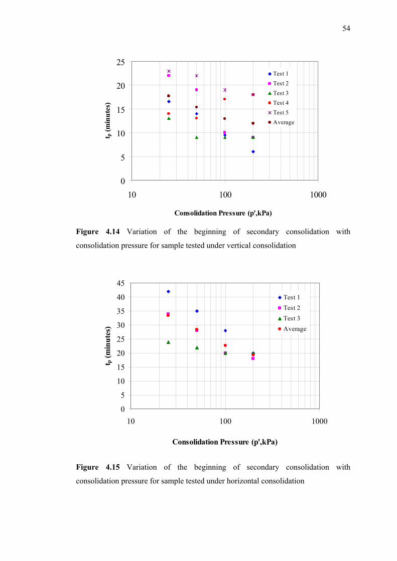
54

0

5

10

15

20

25

10 100 1000

Consolidation Pressure (p',kPa)

t p (m

inut

es)

Test 1Test 2Test 3Test 4Test 5Average

Figure 4.14 Variation of the beginning of secondary consolidation with

consolidation pressure for sample tested under vertical consolidation

0

5

10

15

20

25

30

35

40

45

10 100 1000

Consolidation Pressure (p',kPa)

t p (m

inut

es)

Test 1Test 2Test 3Average

Figure 4.15 Variation of the beginning of secondary consolidation with

consolidation pressure for sample tested under horizontal consolidation

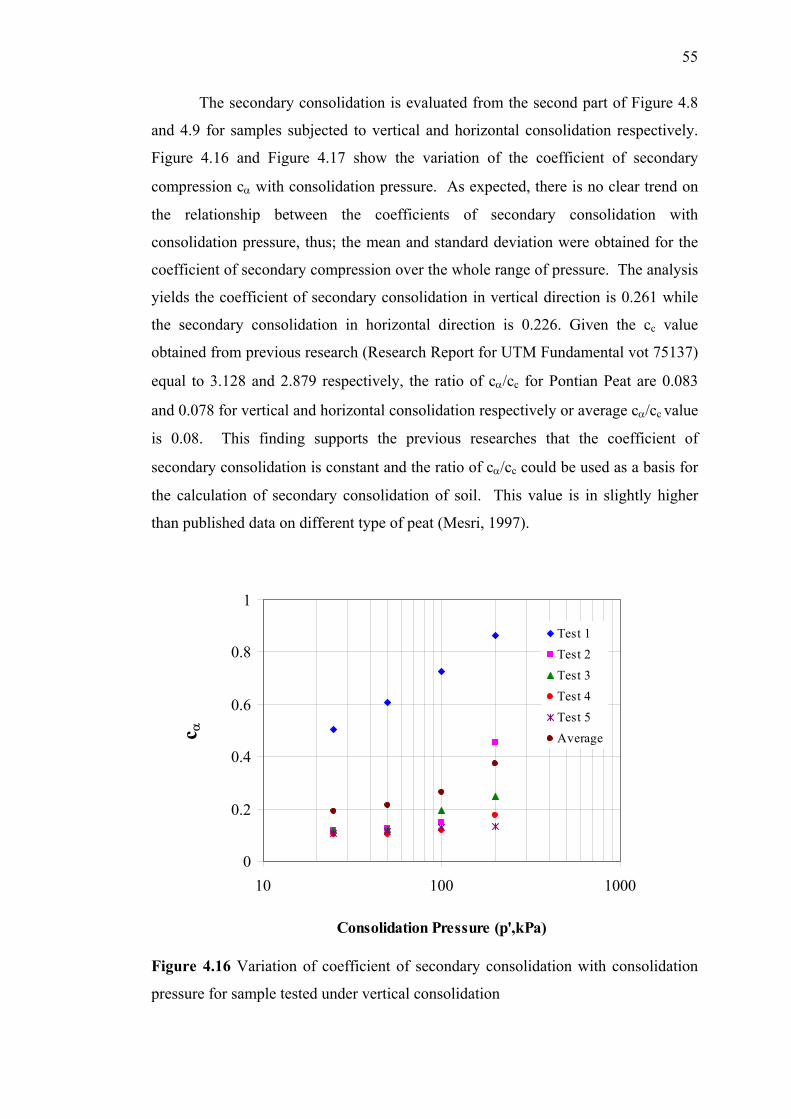
55

The secondary consolidation is evaluated from the second part of Figure 4.8

and 4.9 for samples subjected to vertical and horizontal consolidation respectively.

Figure 4.16 and Figure 4.17 show the variation of the coefficient of secondary

compression cα with consolidation pressure. As expected, there is no clear trend on

the relationship between the coefficients of secondary consolidation with

consolidation pressure, thus; the mean and standard deviation were obtained for the

coefficient of secondary compression over the whole range of pressure. The analysis

yields the coefficient of secondary consolidation in vertical direction is 0.261 while

the secondary consolidation in horizontal direction is 0.226. Given the cc value

obtained from previous research (Research Report for UTM Fundamental vot 75137)

equal to 3.128 and 2.879 respectively, the ratio of cα/cc for Pontian Peat are 0.083

and 0.078 for vertical and horizontal consolidation respectively or average cα/cc value

is 0.08. This finding supports the previous researches that the coefficient of

secondary consolidation is constant and the ratio of cα/cc could be used as a basis for

the calculation of secondary consolidation of soil. This value is in slightly higher

than published data on different type of peat (Mesri, 1997).

0

0.2

0.4

0.6

0.8

1

10 100 1000

Consolidation Pressure (p',kPa)

c α

Test 1Test 2Test 3Test 4Test 5Average

Figure 4.16 Variation of coefficient of secondary consolidation with consolidation

pressure for sample tested under vertical consolidation

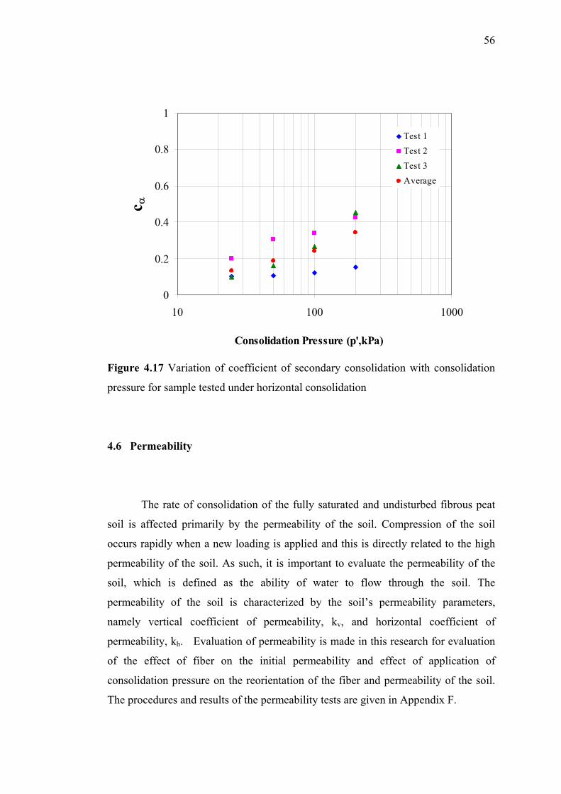
56

0

0.2

0.4

0.6

0.8

1

10 100 1000

Consolidation Pressure (p',kPa)

c αTest 1Test 2Test 3Average

Figure 4.17 Variation of coefficient of secondary consolidation with consolidation

pressure for sample tested under horizontal consolidation

4.6 Permeability

The rate of consolidation of the fully saturated and undisturbed fibrous peat

soil is affected primarily by the permeability of the soil. Compression of the soil

occurs rapidly when a new loading is applied and this is directly related to the high

permeability of the soil. As such, it is important to evaluate the permeability of the

soil, which is defined as the ability of water to flow through the soil. The

permeability of the soil is characterized by the soil’s permeability parameters,

namely vertical coefficient of permeability, kv, and horizontal coefficient of

permeability, kh. Evaluation of permeability is made in this research for evaluation

of the effect of fiber on the initial permeability and effect of application of

consolidation pressure on the reorientation of the fiber and permeability of the soil.

The procedures and results of the permeability tests are given in Appendix F.

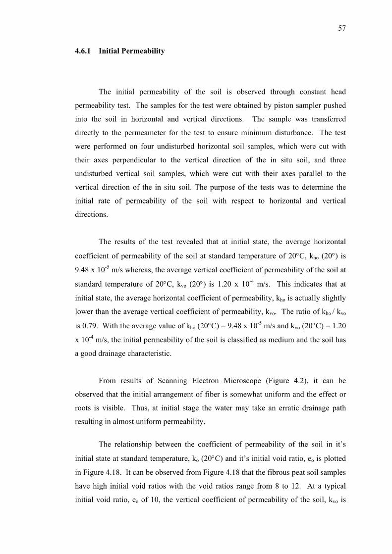
57

4.6.1 Initial Permeability

The initial permeability of the soil is observed through constant head

permeability test. The samples for the test were obtained by piston sampler pushed

into the soil in horizontal and vertical directions. The sample was transferred

directly to the permeameter for the test to ensure minimum disturbance. The test

were performed on four undisturbed horizontal soil samples, which were cut with

their axes perpendicular to the vertical direction of the in situ soil, and three

undisturbed vertical soil samples, which were cut with their axes parallel to the

vertical direction of the in situ soil. The purpose of the tests was to determine the

initial rate of permeability of the soil with respect to horizontal and vertical

directions.

The results of the test revealed that at initial state, the average horizontal

coefficient of permeability of the soil at standard temperature of 20°C, kho (20°) is

9.48 x 10-5 m/s whereas, the average vertical coefficient of permeability of the soil at

standard temperature of 20°C, kvo (20°) is 1.20 x 10-4 m/s. This indicates that at

initial state, the average horizontal coefficient of permeability, kho is actually slightly

lower than the average vertical coefficient of permeability, kvo. The ratio of kho / kvo

is 0.79. With the average value of kho (20°C) = 9.48 x 10-5 m/s and kvo (20°C) = 1.20

x 10-4 m/s, the initial permeability of the soil is classified as medium and the soil has

a good drainage characteristic.

From results of Scanning Electron Microscope (Figure 4.2), it can be

observed that the initial arrangement of fiber is somewhat uniform and the effect or

roots is visible. Thus, at initial stage the water may take an erratic drainage path

resulting in almost uniform permeability.

The relationship between the coefficient of permeability of the soil in it’s

initial state at standard temperature, ko (20°C) and it’s initial void ratio, eo is plotted

in Figure 4.18. It can be observed from Figure 4.18 that the fibrous peat soil samples

have high initial void ratios with the void ratios range from 8 to 12. At a typical

initial void ratio, eo of 10, the vertical coefficient of permeability of the soil, kvo is

58

about 1.32 times higher than the horizontal coefficient of permeability, kho. It can

also be observed from Figure 4.16 that initial permeability of the soil varies from

sample to sample. This shows that the soil is anisotropic and the anisotropy in initial

permeability of the soil results from the natural soil imperfections or discontinuities,

such as root holes, animal burrows, joints, fissures, seams, and soil cracks, that

significantly contribute to high initial permeability of the soil. A significant visual

observation on all the soil samples after the tests is the presence of horizontal as well

as vertical rootlets that create many open voids and channels, and that explain why

the fibrous peat soil is as porous as clean sand.

HorizontalR2 = 0.99

VerticalR2 = 0.96

1.00E-07

1.00E-04

2.00E-04

3.00E-04

4.00E-04

5.00E-04

6.00E-04

7.00E-04

8.00E-04

9.00E-04

1.00E-03

8.00 8.50 9.00 9.50 10.00 10.50 11.00 11.50 12.00

Initial void ratio, e o

Coe

ffic

ient

of p

erm

eabi

lity,

ko (

20癈

) (m

/s)

Figure 4.18: Graph of coefficient of permeability at standard temperature of 20°C,

ko (20°C) versus initial void ratio, eo of the fibrous peat soil samples

4.5.2 Effect of Consolidation Pressure on Permeability

Hydraulic permeability test was carried out at a consolidation pressure of 100

and 200 kPa and an inlet pressure of 90 and 180 kPa on the soil sample. The outlet

pressure was determined by the height of the water collected by a burette connected

to the outlet of water flow from the Rowe consolidometer. The burette has an

internal diameter of 12.19 mm, an external diameter of 15.15 mm and a maximum

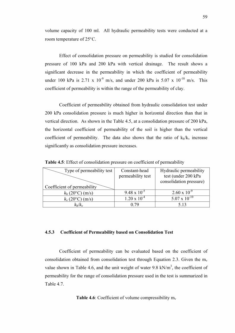
59

volume capacity of 100 ml. All hydraulic permeability tests were conducted at a

room temperature of 25°C.

Effect of consolidation pressure on permeability is studied for consolidation

pressure of 100 kPa and 200 kPa with vertical drainage. The result shows a

significant decrease in the permeability in which the coefficient of permeability

under 100 kPa is 2.71 x 10-9 m/s, and under 200 kPa is 5.07 x 10-10 m/s. This

coefficient of permeability is within the range of the permeability of clay.

Coefficient of permeability obtained from hydraulic consolidation test under

200 kPa consolidation pressure is much higher in horizontal direction than that in

vertical direction. As shown in the Table 4.5, at a consolidation pressure of 200 kPa,

the horizontal coefficient of permeability of the soil is higher than the vertical

coefficient of permeability. The data also shows that the ratio of kh/kv increase

significantly as consolidation pressure increases.

Table 4.5: Effect of consolidation pressure on coefficient of permeability

Type of permeability test Coefficient of permeability

Constant-head permeability test

Hydraulic permeability test (under 200 kPa

consolidation pressure)

kh (20°C) (m/s) 9.48 x 10-5 2.60 x 10-9

kv (20°C) (m/s) 1.20 x 10-4 5.07 x 10-10

kh/kv 0.79 5.13

4.5.3 Coefficient of Permeability based on Consolidation Test

Coefficient of permeability can be evaluated based on the coefficient of

consolidation obtained from consolidation test through Equation 2.3. Given the mv

value shown in Table 4.6, and the unit weight of water 9.8 kN/m3, the coefficient of

permeability for the range of consolidation pressure used in the test is summarized in

Table 4.7.

Table 4.6: Coefficient of volume compressibility mv

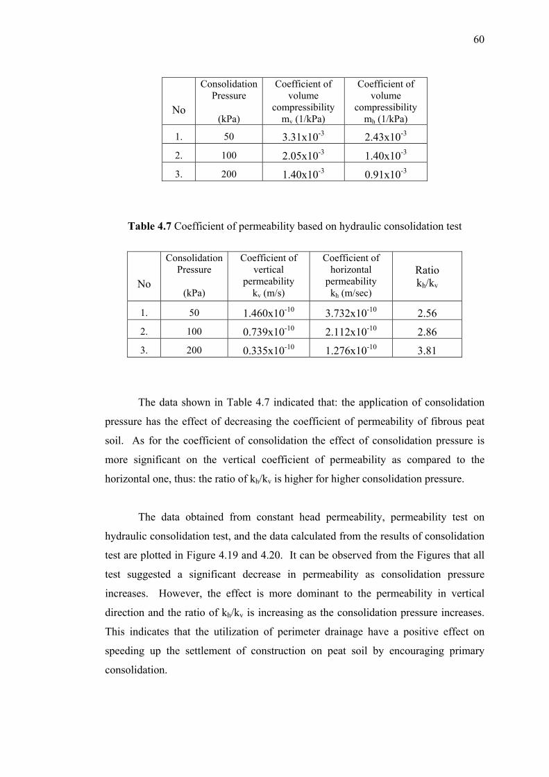
60

No

ConsolidationPressure

(kPa)

Coefficient of volume

compressibility mv (1/kPa)

Coefficient of volume

compressibility mh (1/kPa)

1. 50 3.31x10-3 2.43x10-3

2. 100 2.05x10-3 1.40x10-3

3. 200 1.40x10-3 0.91x10-3

Table 4.7 Coefficient of permeability based on hydraulic consolidation test

No

Consolidation Pressure

(kPa)

Coefficient of vertical

permeability kv (m/s)

Coefficient of horizontal

permeability kh (m/sec)

Ratio kh/kv

1. 50 1.460x10-10 3.732x10-10 2.56 2. 100 0.739x10-10 2.112x10-10 2.86 3. 200 0.335x10-10 1.276x10-10 3.81

The data shown in Table 4.7 indicated that: the application of consolidation

pressure has the effect of decreasing the coefficient of permeability of fibrous peat

soil. As for the coefficient of consolidation the effect of consolidation pressure is

more significant on the vertical coefficient of permeability as compared to the

horizontal one, thus: the ratio of kh/kv is higher for higher consolidation pressure.

The data obtained from constant head permeability, permeability test on

hydraulic consolidation test, and the data calculated from the results of consolidation

test are plotted in Figure 4.19 and 4.20. It can be observed from the Figures that all

test suggested a significant decrease in permeability as consolidation pressure

increases. However, the effect is more dominant to the permeability in vertical

direction and the ratio of kh/kv is increasing as the consolidation pressure increases.

This indicates that the utilization of perimeter drainage have a positive effect on

speeding up the settlement of construction on peat soil by encouraging primary

consolidation.

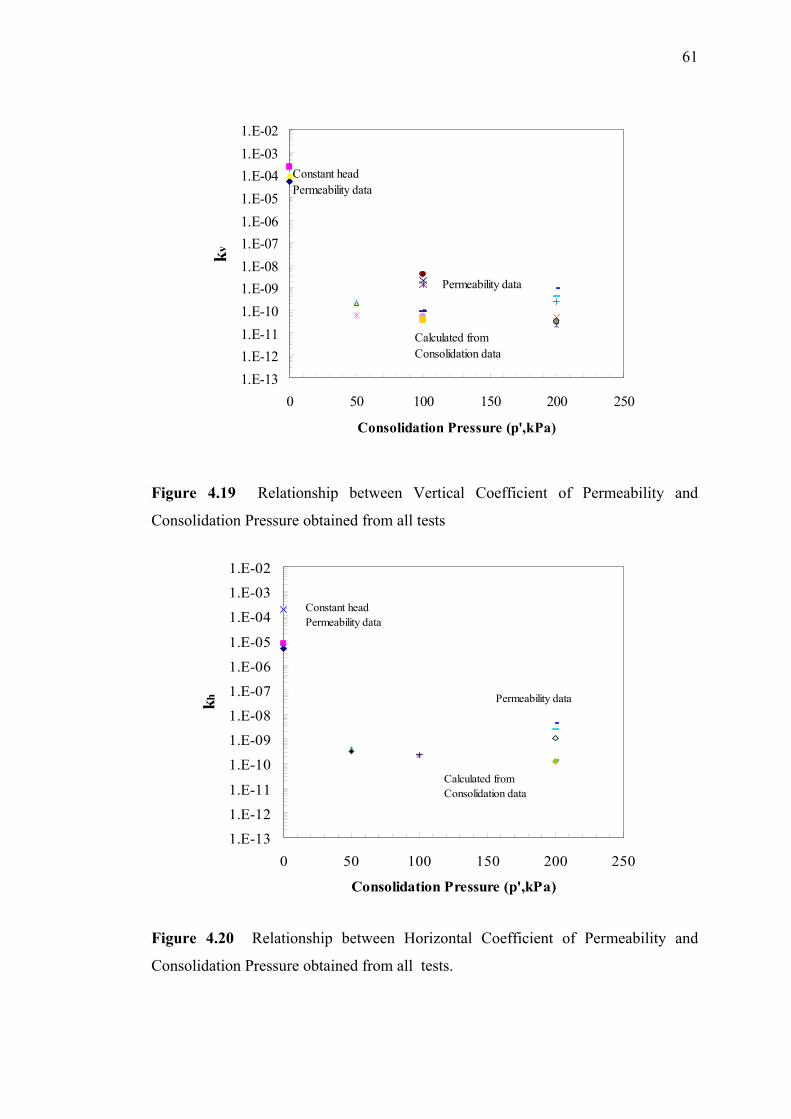
61

1.E-131.E-121.E-111.E-101.E-091.E-081.E-071.E-061.E-051.E-041.E-031.E-02

0 50 100 150 200 250

Consolidation Pressure (p',kPa)

kv

Constant headPermeability data

Calculated fromConsolidation data

Permeability data

Figure 4.19 Relationship between Vertical Coefficient of Permeability and

Consolidation Pressure obtained from all tests

1.E-13

1.E-12

1.E-11

1.E-10

1.E-09

1.E-08

1.E-07

1.E-06

1.E-05

1.E-04

1.E-03

1.E-02

0 50 100 150 200 250

Consolidation Pressure (p',kPa)

kh Permeability data

Calculated fromConsolidation data

Constant headPermeability data

Figure 4.20 Relationship between Horizontal Coefficient of Permeability and

Consolidation Pressure obtained from all tests.

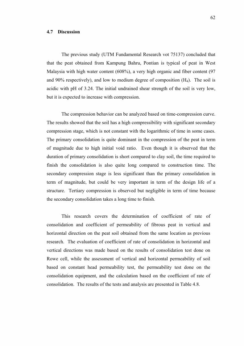
62

4.7 Discussion

The previous study (UTM Fundamental Research vot 75137) concluded that

that the peat obtained from Kampung Bahru, Pontian is typical of peat in West

Malaysia with high water content (608%), a very high organic and fiber content (97

and 90% respectively), and low to medium degree of composition (H4). The soil is

acidic with pH of 3.24. The initial undrained shear strength of the soil is very low,

but it is expected to increase with compression.

The compression behavior can be analyzed based on time-compression curve.

The results showed that the soil has a high compressibility with significant secondary

compression stage, which is not constant with the logarithmic of time in some cases.

The primary consolidation is quite dominant in the compression of the peat in term

of magnitude due to high initial void ratio. Even though it is observed that the

duration of primary consolidation is short compared to clay soil, the time required to

finish the consolidation is also quite long compared to construction time. The

secondary compression stage is less significant than the primary consolidation in

term of magnitude, but could be very important in term of the design life of a

structure. Tertiary compression is observed but negligible in term of time because

the secondary consolidation takes a long time to finish.

This research covers the determination of coefficient of rate of

consolidation and coefficient of permeability of fibrous peat in vertical and

horizontal direction on the peat soil obtained from the same location as previous

research. The evaluation of coefficient of rate of consolidation in horizontal and

vertical directions was made based on the results of consolidation test done on

Rowe cell, while the assessment of vertical and horizontal permeability of soil

based on constant head permeability test, the permeability test done on the

consolidation equipment, and the calculation based on the coefficient of rate of

consolidation. The results of the tests and analysis are presented in Table 4.8.

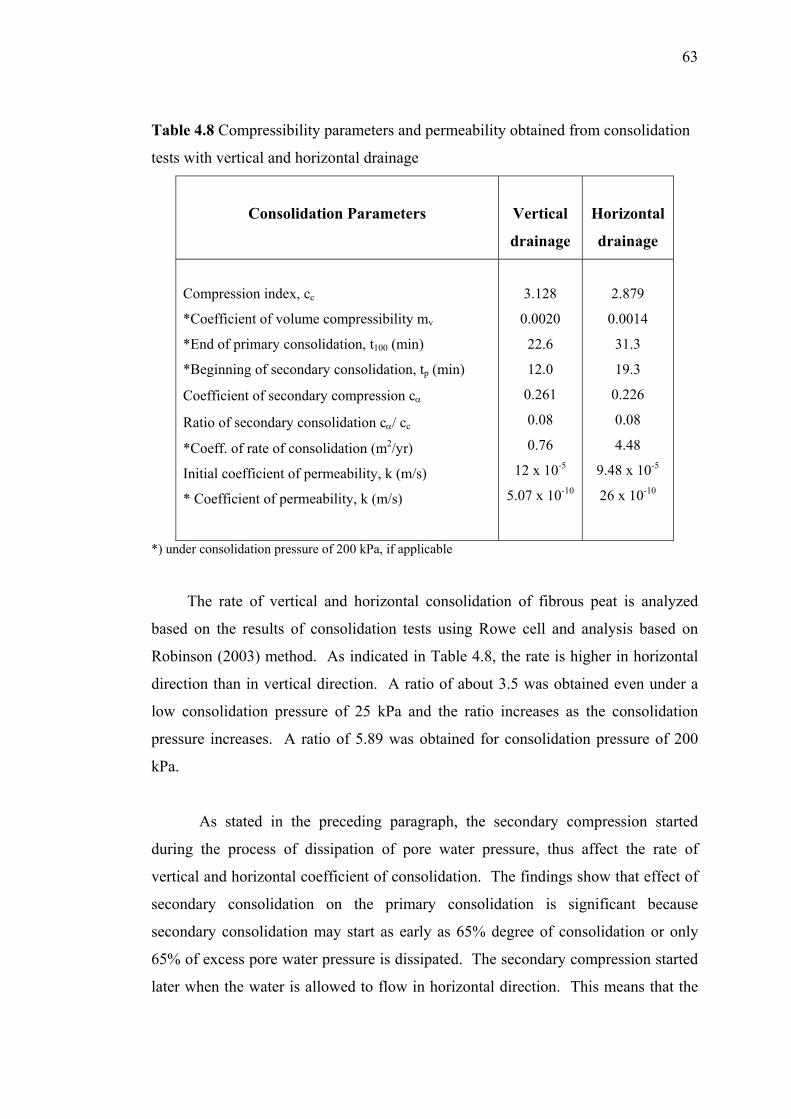
63

Table 4.8 Compressibility parameters and permeability obtained from consolidation

tests with vertical and horizontal drainage

Consolidation Parameters

Vertical

drainage

Horizontal

drainage

Compression index, cc

*Coefficient of volume compressibility mv

*End of primary consolidation, t100 (min)

*Beginning of secondary consolidation, tp (min)

Coefficient of secondary compression cα

Ratio of secondary consolidation cα/ cc

*Coeff. of rate of consolidation (m2/yr)

Initial coefficient of permeability, k (m/s)

* Coefficient of permeability, k (m/s)

3.128

0.0020

22.6

12.0

0.261

0.08

0.76

12 x 10-5

5.07 x 10-10

2.879

0.0014

31.3

19.3

0.226

0.08

4.48

9.48 x 10-5

26 x 10-10

*) under consolidation pressure of 200 kPa, if applicable

The rate of vertical and horizontal consolidation of fibrous peat is analyzed

based on the results of consolidation tests using Rowe cell and analysis based on

Robinson (2003) method. As indicated in Table 4.8, the rate is higher in horizontal

direction than in vertical direction. A ratio of about 3.5 was obtained even under a

low consolidation pressure of 25 kPa and the ratio increases as the consolidation

pressure increases. A ratio of 5.89 was obtained for consolidation pressure of 200

kPa.

As stated in the preceding paragraph, the secondary compression started

during the process of dissipation of pore water pressure, thus affect the rate of

vertical and horizontal coefficient of consolidation. The findings show that effect of

secondary consolidation on the primary consolidation is significant because

secondary consolidation may start as early as 65% degree of consolidation or only

65% of excess pore water pressure is dissipated. The secondary compression started

later when the water is allowed to flow in horizontal direction. This means that the

64

effect of secondary compression on primary consolidation can be minimized by

providing vertical drain in fibrous peat deposit.

The ratio of secondary compression to the compression index is proofed to be

almost constant with consolidation pressure as well as the direction of drainage. The

study suggests a ratio of 0.08 which is slightly higher than published data (Ajlouni,

2002). This might be due to the high fiber content of the soil.

Initial permeability of the peat is very high and it is comparable to sand.

However, the data also showed that the permeability is highly affected by

compression or reduction in void ratio. The coefficient of permeability decreases

drastically as consolidation increases. The initial permeability is 1.2 x 10-4 m/s,

while the coefficient of permeability under consolidation pressure of 200 kPa is

found as 5.07 x 10-10 m/s. The lower coefficient of permeability was assessed from

the results of consolidation test through cv values. For this case, the coefficient of

permeability calculated based on the coefficient of rate of consolidation are 7.39 x 10 -11 m/s 3.35 x 10 -11 m/s for the consolidation pressure of 100 and 200 kPa

respectively.

Permeability of the fibrous peat soil is affected by the arrangement fiber in the

soil mass. Scanning Electron micrograph was taken on samples of fibrous peat cut in

vertical and horizontal direction under various consolidation pressures. It is the

objective of the research to evaluate the effect of fiber orientation and to compare the

vertical and horizontal coefficient of permeability, (kh and kv) of fibrous peat soil

under a range of consolidation pressure. Comparison of the results of SEM on

samples cut in vertical and horizontal direction demonstrates the difference in the

fiber arrangement in both direction and the effect of application of consolidation

pressure on the fiber arrangement. It is clear that the effect of consolidation pressure

can be reduced if the water is allowed to flow in horizontal direction. The ratio of

kh/kv increases from 0.79 for initial condition to about 5 under consolidation pressure

of 200 kPa.

65

The final objective of the study was to outline the use of knowledge of

horizontal coefficient of consolidation, ch on the development of soil improvement

method for construction on fibrous peat soil. In general, the results of the study

indicate that the utilization of vertical drainage on the perimeter improves the

compressibility of fibrous peat soil in terms of both primary consolidation and

secondary compression. The coefficient of rate of consolidation increases

significantly by application of the perimeter drainage and it is not much affected by

the application of consolidation pressure. The rate of secondary consolidation is also

improved by the application of vertical drainage even though the time needed to

finish consolidation is much slower due to the length of drainage path. This can be

improved by designing an optimum distance of vertical drainage. The effect of

secondary consolidation on primary consolidation stage can also be improved by the

utilization of vertical drain.

The results of this study suggested that sand column or other means of

vertical drainage could be an effective method of soil improvement for fibrous peat

soil. Besides reducing the compressibility of the soil and increasing the rate of

primary consolidation, the drainage can have a positive effect on increasing the shear

strength of the soil, thus; the height of fill can be improved. The method should be

combined with confinement because the most critical problem involving peat soil is

lateral spreading of the soil. This method has been applied successfully for peat soil

deposits in Japan and many other countries.

66

CHAPTER 5

CONCLUSIONS AND RECOMMENDATION FOR FUTURE STUDY

5.1 Conclusions

The first objective of the study is to determine the horizontal coefficient of

consolidation on Rowe consolidation test, and how it compared with the vertical

coefficient of consolidation. It is found that the coefficient of rate of consolidation is

higher in the horizontal direction than in the vertical direction.

The effect of secondary consolidation on the primary consolidation is

significant, thus: it is recommended to perform large strain consolidation test on

Rowe cell. The secondary compression is less dominant when the soil is subjected to

horizontal drainage, thus utilization of vertical drainage will reduce the secondary

compression. Furthermore the study indicated that the coefficient of secondary

consolidation decreases when water is allowed to flow in horizontal direction. The

cα/cc ratio obtained from this study is 0.08 which is in higher end of the range

suggested by previous researchers.

Application of consolidation pressure has the effect of decreasing the

coefficient of consolidation; however the horizontal rate of consolidation decreases

in a slower rate than the vertical coefficient of consolidation due to the

rearrangement of the fiber in the soil. The ratio of ch/cv is increasing from 3.5 to 6.0

for consolidation pressure of 25 to 200 kPa.

67

The fourth objective of the research is to evaluate the effect of fiber orientation

and to compare the vertical and horizontal coefficient of permeability, (kh and kv) of

fibrous peat soil under a range of consolidation pressure. Results show that the ratio

of kh/kv increases from 0.79 for initial condition to about 5 under consolidation

pressure of 200 kPa. Thus the permeability of the soil in horizontal direction is not

greatly affected by the application of consolidation pressure.

The final objective of the research was to outline the use of knowledge of

horizontal coefficient of consolidation, ch on the development of soil improvement

method for construction on fibrous peat soil. The results shows that utilization of

perimeter drainage has a positive effect on speeding up the primary consolidation

process, thus the post-construction estimation of the settlement could be made based

only on the secondary compression.

5.2 Recommendation for Future Study

The research conducted in this study has been limited to the laboratory

evaluation of compressibility characteristics of fibrous peat soil. Results have shown

that utilization of perimeter or any form of vertical drainage could be a good

improvement method when construction is to take place on fibrous peat deposit. The

method has been applied successfully for peat soil deposits in Japan and many other

countries. The method has the advantage of increasing shear strength and at the

same time increasing the rate of primary consolidation process.

Further study involving field investigation on the fibrous peat soil needs to be

done to justify the laboratory investigation on the soil from this study and to test the

suitability of the method. An evaluation on the increase in shear strength due to

application of consolidation pressure and draining process is recommended as an

extension of this research because the shear strength of the soil determine the amount

of fill that could be placed to induce consolidation and compression.

68

REFERENCES

Adams, J. (1965). The Engineering Behavior of a Canadian Muskeg. Proc., 6th Int.

Conf. Soil Mech. Found. Engrg. Montreal, Canada, 1: 3-7.

Ajlouni, M.A. (2000) Geotechnical Properties of Peat and RelatedEengineering

Problems. Thesis. University of Illinois at Urbana-Champaign.

American Society for Testing and Materials. (1994) Annual Book of ASTM Standard.

Vol. 04.08 and 04.09

Asaoka, A. (1978). Observational Procedure of Settlement Prediction. Soils and

Foundation, 18(4):87-101.

British Standards Institution. (1981). Methods of Test for Soils for Civil Engineering

Purposes. London, BS 1377.

Clarke, B. G., Carter, J. P. and Wroth, C. P. (1979). In Situ Determination of the

ConsolidationCharacteristics of Saturated Clays.Proc. 7th Eur. Conf. Soil Mech.,

Brighton, 2:207-211 .

Colley, B. E. (1950). Construction of Highways Over Peat and Muck Areas.

American Highway, 29(1): 3-7.

Colleselli, F., Cortellazzo, G., and Cola, S., (2000). Laboratory Testing of Italian

Peat Soils, Geotechnics of High Water Content Materials, ASTM STP 1374, Edil,

T.B., and Fox, P.J. (Eds.), American Society for Testing and Materials, West

Conshohocken, PA.

Dhowian, A. W. and Edil, T. B. (1980). Consolidation Behavior of Peats. Geotech.

Testing J., 3(3): 105-114.

Edil, T.B. and A. W. Dhowian. (1981). At-rest Lateral Pressure of Peat Soils. Conf.

on Sedimentation and Consolidation Model, ASCE, San Fransisco, 411 – 424.

Edil, T.B. (2001) Site Characterization in Peat and Organic Soils. In Proceeding of

the International Conference on In Situ Measurement of Soil Properties and Case

Histories, 49-59, Bali, Indonesia.

69

Edil, T.B. (2003). Recent Advances in Geotechnical Characterization and

Construction Over Peats and Organic Soils. Putrajaya (Malaysia): 2nd

International Conferences in Soft Soil Engineering and Technology.

Escario, V. and Uriel, S. (1961). Detremining the Coefficient of Consolidation and

Horizontal Permeability by Radial Drainage. 5th ICSMFE, 1:83-87.

Fox, P.J., and Edil, T.B. (1966). Effects of Stress and Temperature on Secondary

Compression of Peat. Canadian Geotechnical Journal. 33(3): 405-415.

Hanrahan, E. T. (1954). An Investigation of Some Physical Properties of Peat."

Geotechnique, London, England, 4(2): 108-123.

Hartlen, J. and J. Wolski. (1996). Embankments on Organic Soils. Developemnet in

Geotechnical Engineering, Elsevier. 425.

Head, K.H., (1981). Manual of Soil Laboratory Testing, Volume 1,2, and 3. Pentech

Press, London.

Head, K.H. (1982). Manual of Soil Laboratory Testing, Volume 2: Permeability,

Shear Strength and Compressibility Tests. London: Pentech Press Limited.

Head, K.H. (1986). Manual of Soil Laboratory Testing, Volume 3: Effective Stress

Tests. London: Pentech Press Limited.

Hillis, S. F.and C. O. Brawner, (1961). The Compressibility of Peat with references

to Construction of Major Highways in B. C. Proc. 7th Muskeg Res. Conf., Ottawa.

Huat, Bujang, B.K., (2004) Organic and Peat Soil Engineering. Univ. Putra

Malaysia Press.

Hobbs, N. B. (1986). Mire Morphology and the Properties and Behaviour of Some

British and Foreign Peats. Q. I Eng. Geol., London, 19(1): 7-80.

Holtz, R.D. and Kovacs, W.D. (1981). An Introduction to Geotechnical Engineering.

Prentice-Hall, Inc., Englewood Cliffs, New Jersey.

Karlsson, R. and Hansbo, S. (1981). (In Collaboration with the Laboratory

Committee of the Swedish Geotechnical Society). Soil Classification and

Identification. Swedish Council for Building Research. D8:81. Stockholm.

Kogure, K., Yamaguchi, H., and Shogaki, T. (1993). Physical and Pore Properties

of Fibrous Peat Deposit. Singapore: 11th Southeast Asian Geotechnical

Conference. 1993.

Lan, l.T. (1992). A Model for One-dimensional Compression of Peat. Ph.D. thesis.

University of Wisconsin, Madison, U.S.A.

70

Landva, A. O., Pheeney, P. E. and Mersereau, D. E. (1983). Undisturbed Sampling

of peat. Testing of Peat and Organic Soils, ASTM STP 820, 141-156.

Landva,A.O. and La Rochelle, P. (1983). Compressibility and Shear Characteristics

of Radforth Peats, Testing of Peat and Organic Soils, ASTM STP, 820: 157-191.

Lea, N., D. and Browner, C. 0. (1963). Highway Design and Construction Over Peat

Deposits in the Lower British Colombia. Highway Research Record, (7): 1-32.

Leonards, G.A. and P. Girault. (1961). A Study of The One-dimensional

Consolidation Test.Proceeding 9th ICSMFE, Paris, 1:116-130.

Mesri, G., Stark, T. D. and Chen, C. S. (1994). Cc/Cα Concept Applied to

Compression of Peat. Discussion, J. of Geotech. Engrg., ASCE, 118(8): 764-766.

Mesri, G., T.D. Statark, M.A. Ajlouni and C. S. Chen (1997). Secondary

Compression of Peat With or Without Surcharging. J. Geotech. Geoev. Engr.

123(5): 411-421.

Miyakawa, J. (1960). Soils Engineering Research on Peats Alluvia. Reports 1-3.

Civil Enggrg. Research Institute. Hokkaido Development Bureau Bulletin No. 20

Mokhtar, N.E. (1998). Perbedaan Perilaku Teknis Tanah Lempung dan Tanah

Gambut (Peat Soil), Jurnal Geoteknik, Himpunan Ahli Teknik Tanah Indonesia,

3(1): 16-34.

Muskeg Engineering Handbook. (1969). I.C. Macfarlane. Univ of Toronto Press.

Nurly Gofar and Yulindasari Sutejo. (2005). Engineering Properties of Fibrous Peat,

Proc. Seminar Penyelidikan Kej. Awam (SEPKA), Johor Bahru. 119-129.

Noto, Shigeyuki. (1991). Peat Engineering Handbook. Civil Engineering Research

Institute, Hokkaido development Agency, Prime Minister’s Office, Japan.

Robinson, R. G. (1997). Determination of Radial Coefficient of Consolidation by the

Inflection Point Method, Geotechnique, 47(5): 1079-1081.

Robinson, R. G. (2003). A Study on the Beginning of Secondary Compression of

Soils. Journal of Testing and Evaluation. 31(5): 1-10.

Rowe, P.W. and Barden, L. (1966). A New Consolidation Cell. Geotechnique. 16:

162-169.

Tortensson, B. A. (1975). The Pore Pressure Sounding Instrument. Proceeding ASCE

Speciality Conference on In Situ Measurement of Soil Properties. Raleigh 2. New

York. American Society of Civil Engineering. 48-54.

Wilkinson,W. B. (1968). Constan Head In Situ Permeability Tests in Clay Strata.

Geotechnique. 18: 172-194.

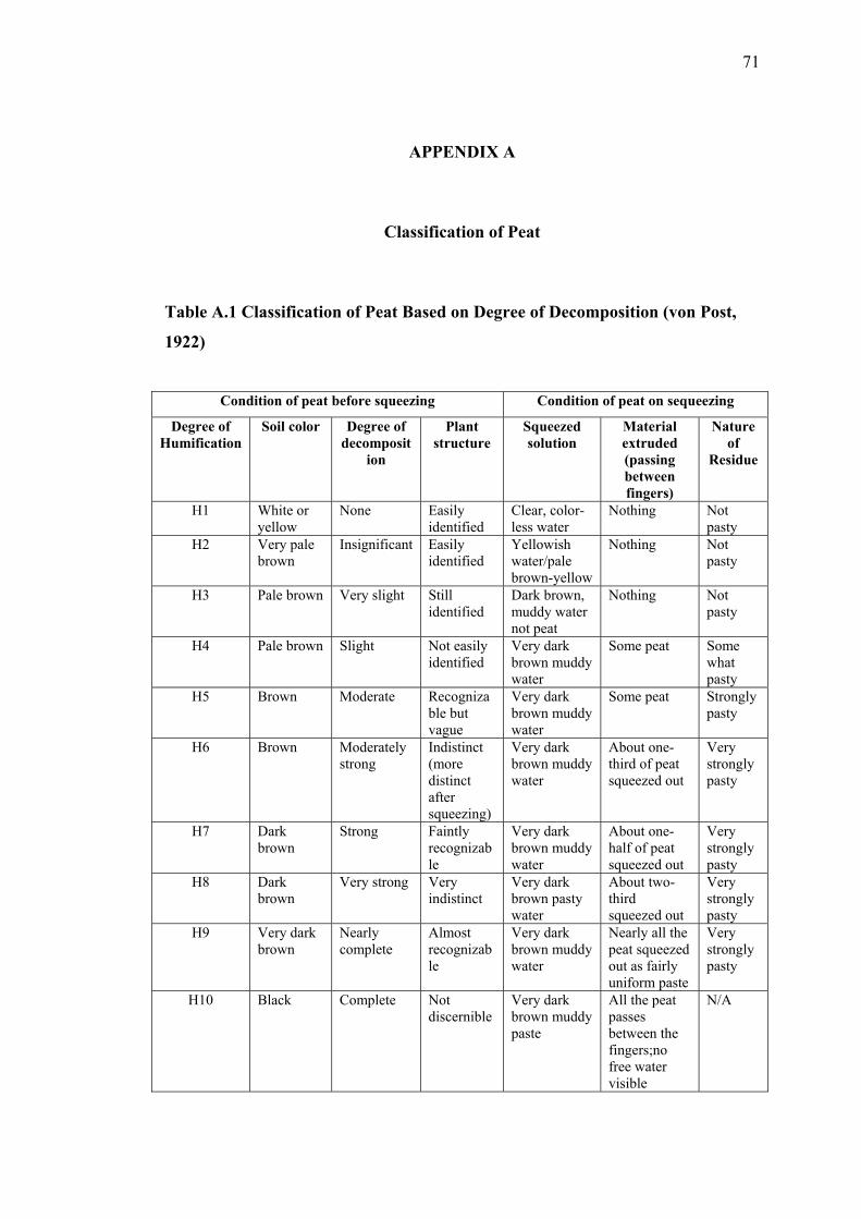
71

APPENDIX A

Classification of Peat

Table A.1 Classification of Peat Based on Degree of Decomposition (von Post,

1922)

Condition of peat before squeezing Condition of peat on sequeezing

Degree of Humification

Soil color Degree of decomposit

ion

Plant structure

Squeezed solution

Material extruded (passing between fingers)

Nature of

Residue

H1 White or yellow

None Easily identified

Clear, color-less water

Nothing Not pasty

H2 Very pale brown

Insignificant Easily identified

Yellowish water/pale brown-yellow

Nothing Not pasty

H3 Pale brown Very slight Still identified

Dark brown, muddy water not peat

Nothing Not pasty

H4 Pale brown Slight Not easily identified

Very dark brown muddy water

Some peat Some what pasty

H5 Brown Moderate Recognizable but vague

Very dark brown muddy water

Some peat Stronglypasty

H6 Brown Moderately strong

Indistinct (more distinct after squeezing)

Very dark brown muddy water

About one-third of peat squeezed out

Very stronglypasty

H7 Dark brown

Strong Faintly recognizable

Very dark brown muddy water

About one-half of peat squeezed out

Very stronglypasty

H8 Dark brown

Very strong Very indistinct

Very dark brown pasty water

About two-third squeezed out

Very stronglypasty

H9 Very dark brown

Nearly complete

Almost recognizable

Very dark brown muddy water

Nearly all the peat squeezed out as fairly uniform paste

Very stronglypasty

H10 Black Complete Not discernible

Very dark brown muddy paste

All the peat passes between the fingers;no free water visible

N/A

72

Table A.2 Clasification of Peat based on organic and fiber content

Classification peat soil based on ASTM standards

Fibric : Peat with greater than 67 % fibers

Hemic : Peat with between 33 % and 67 % fibers

Fiber Content

(ASTM D1997)

Sapric : Peat with less than 67 % fibers

Low Ash : Peat with less than 5 % ash

Medium Ash : Peat with between 5% and 15 % ash

Ash Content

(ASTM D2974)

High Ash : Peat with more than 15 % ash

Highly Acidic : Peat with a pH less than 4.5

Moderately Acidic : Peat with a pH between 4.5 and 5.5

Moderately Acidic : Peat with a pH between 4.5 and 5.5

Slighly Acidic : Peat with a pH greater than 5.5 and less than 7

Acidity

(ASTM D2976)

Basic : Peat with a pH equal or greater than 7

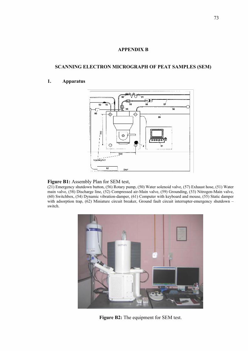
73

APPENDIX B

SCANNING ELECTRON MICROGRAPH OF PEAT SAMPLES (SEM)

1. Apparatus

Figure B1: Assembly Plan for SEM test, (21) Emergency shutdown button, (56) Rotary pump, (50) Water solenoid valve, (57) Exhaust hose, (51) Water main valve, (58) Discharge line, (52) Compressed air-Main valve, (59) Grounding, (53) Nitrogen-Main valve, (60) Switchbox, (54) Dynamic vibration-damper, (61) Computer with keyboard and mouse, (55) Static damper with adsorption trap, (62) Miniature circuit breaker, Ground fault circuit interrupter-emergency shutdown –switch.

Figure B2: The equipment for SEM test.

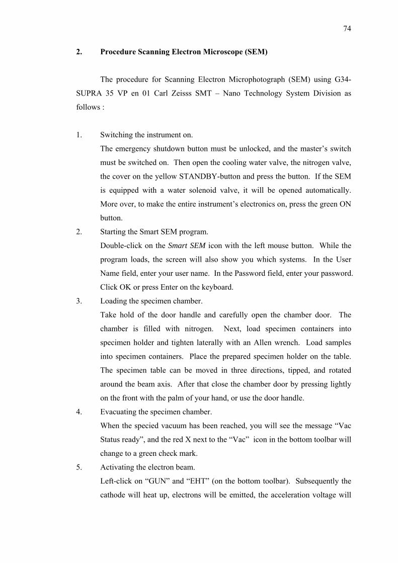
74

2. Procedure Scanning Electron Microscope (SEM)

The procedure for Scanning Electron Microphotograph (SEM) using G34-

SUPRA 35 VP en 01 Carl Zeisss SMT – Nano Technology System Division as

follows :

1. Switching the instrument on.

The emergency shutdown button must be unlocked, and the master’s switch

must be switched on. Then open the cooling water valve, the nitrogen valve,

the cover on the yellow STANDBY-button and press the button. If the SEM

is equipped with a water solenoid valve, it will be opened automatically.

More over, to make the entire instrument’s electronics on, press the green ON

button.

2. Starting the Smart SEM program.

Double-click on the Smart SEM icon with the left mouse button. While the

program loads, the screen will also show you which systems. In the User

Name field, enter your user name. In the Password field, enter your password.

Click OK or press Enter on the keyboard.

3. Loading the specimen chamber.

Take hold of the door handle and carefully open the chamber door. The

chamber is filled with nitrogen. Next, load specimen containers into

specimen holder and tighten laterally with an Allen wrench. Load samples

into specimen containers. Place the prepared specimen holder on the table.

The specimen table can be moved in three directions, tipped, and rotated

around the beam axis. After that close the chamber door by pressing lightly

on the front with the palm of your hand, or use the door handle.

4. Evacuating the specimen chamber.

When the specied vacuum has been reached, you will see the message “Vac

Status ready”, and the red X next to the “Vac” icon in the bottom toolbar will

change to a green check mark.

5. Activating the electron beam.

Left-click on “GUN” and “EHT” (on the bottom toolbar). Subsequently the

cathode will heat up, electrons will be emitted, the acceleration voltage will

75

be on, and the image on the screen will turn lighter. If the focus is (by chance)

already correct, the contours of the specimen will appear.

6. Focusing the electron beam.

The objective focuses the electron beam on the surface of the specimen. The

specimen must be placed in the correct position under the electron beam

before you bring it into focus. If the image is not sharp enough, you will

need to make further adjustments.

7. Modifying the image.

The Smart SEM program has many functions to help you obtain the desired

results. Information of interest can be accessed via Windows help, program

help, or context-based help.

8. VP-Mode.

When examining non- or only slightly conductive preparations, charges can

be induced on their surfaces, which are difficult or impossible to divert and

which result in an altered image. In VP-Mode, these surface charges are

avoided or reduced and high-quality images can be produced, even from such

preparations.

9. Finishing examination of a specimen.

You can save or print out an image if it meets your quality requirements. If

you did not order a printer with your instrument, you can move the file to

another computer with a printer and print it out from there.

10. Placing the SEM in standby mode.

Standby mode is the normal status for the SEM once you have finished

examining a specimen. The cathode will continue to heat, and the vacuum

pump will evacuate the electro-optic column and the specimen chamber.

11. Switching off the SEM.

The SEM must be shut down for maintenance, repairs, if the instrument will

not be used for an extended period of time or in case of an emergency.

12. Shutting down the SEM completely.

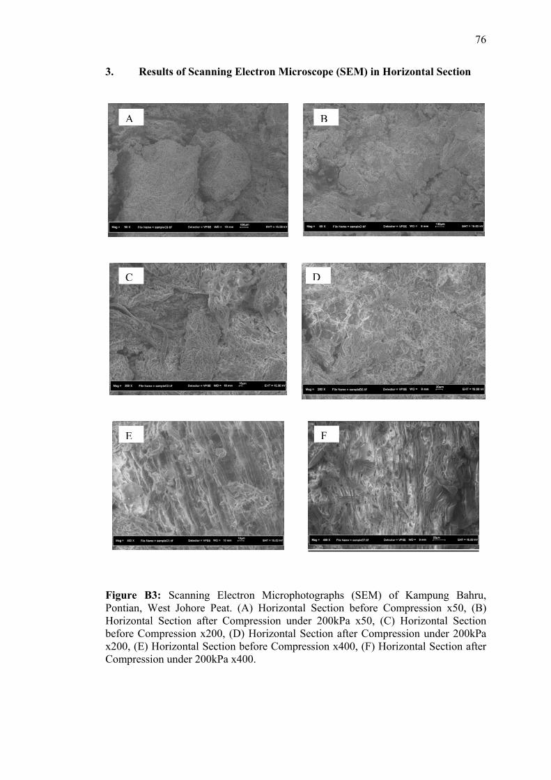
76

3. Results of Scanning Electron Microscope (SEM) in Horizontal Section

A B

DC

FE

Figure B3: Scanning Electron Microphotographs (SEM) of Kampung Bahru, Pontian, West Johore Peat. (A) Horizontal Section before Compression x50, (B) Horizontal Section after Compression under 200kPa x50, (C) Horizontal Section before Compression x200, (D) Horizontal Section after Compression under 200kPa x200, (E) Horizontal Section before Compression x400, (F) Horizontal Section after Compression under 200kPa x400.

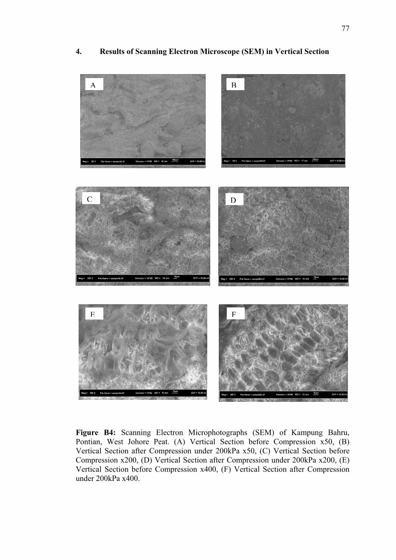
77

4. Results of Scanning Electron Microscope (SEM) in Vertical Section

A B

C

E

Figure B4: Scanning Electron MicrophotoPontian, West Johore Peat. (A) Vertical SeVertical Section after Compression under 200Compression x200, (D) Vertical Section after Vertical Section before Compression x400, (Funder 200kPa x400.

D

g

C

F

raphs (SEM) of Kampung Bahru, ction before Compression x50, (B) kPa x50, (C) Vertical Section before

ompression under 200kPa x200, (E) ) Vertical Section after Compression

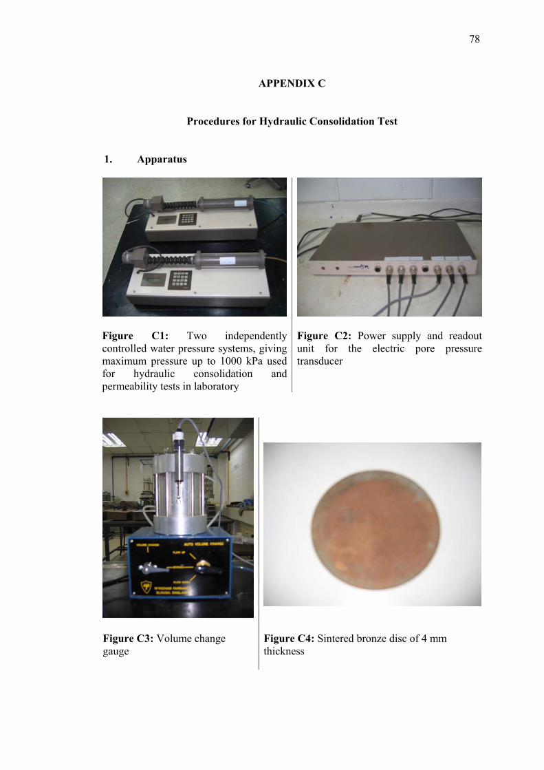
78

APPENDIX C

Procedures for Hydraulic Consolidation Test 1. Apparatus

Figure C1: Two independently controlled water pressure systems, giving maximum pressure up to 1000 kPa used for hydraulic consolidation and permeability tests in laboratory

Figure C2: Power supply and readout unit for the electric pore pressure transducer

Figure C3: Volume change gauge

Figure C4: Sintered bronze disc of 4 mm thickness

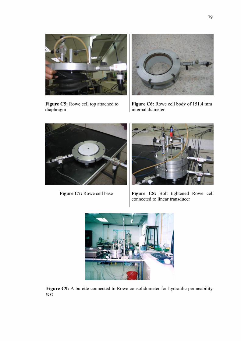
79

Figure C5: Rowe cell top attached to diaphragm

Figure C6: Rowe cell body of 151.4 mm internal diameter

Figure C7: Rowe cell base

Figure C8: Bolt tightened Rowe cell connected to linear transducer

Figure C9: A burette connected to Rowe consolidometer for hydraulic permeability test

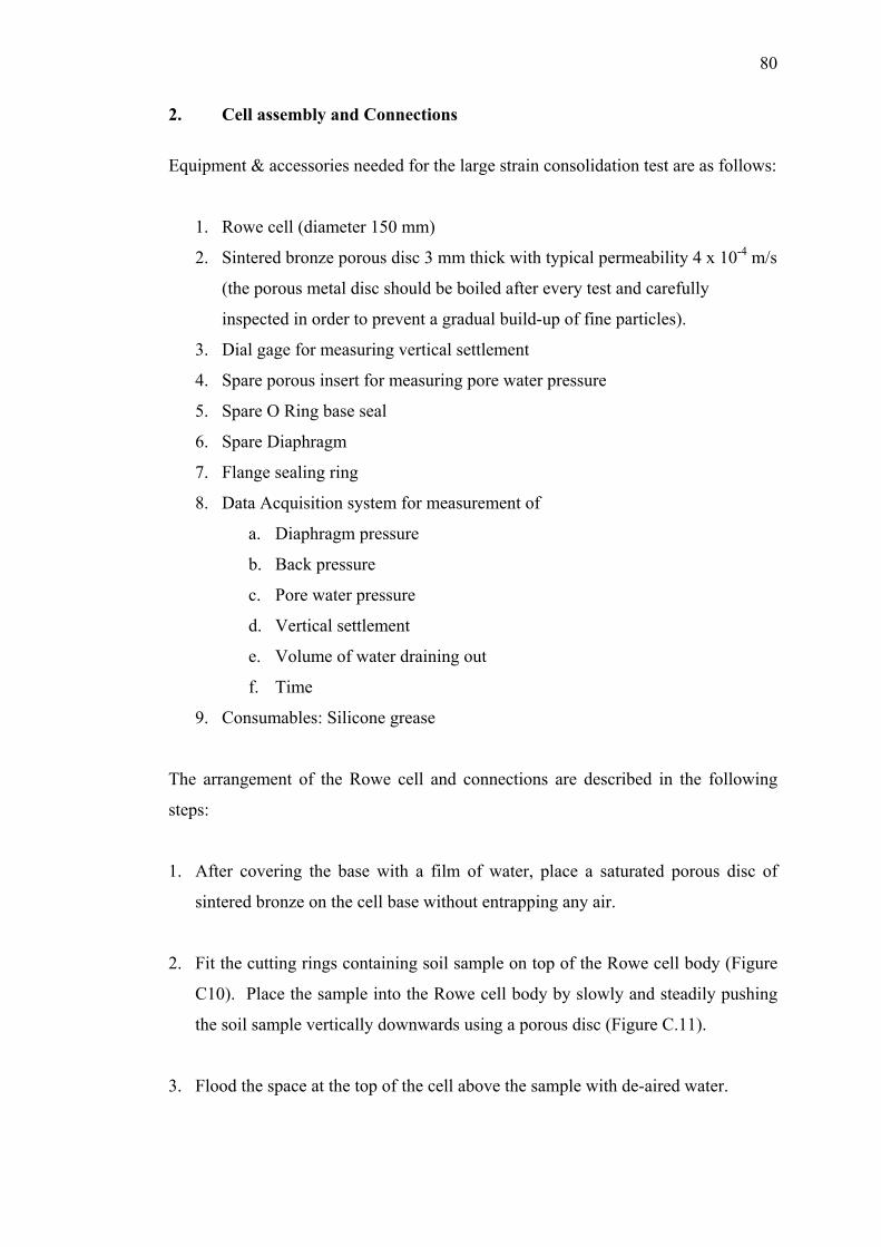
80

2. Cell assembly and Connections

Equipment & accessories needed for the large strain consolidation test are as follows:

1. Rowe cell (diameter 150 mm)

2. Sintered bronze porous disc 3 mm thick with typical permeability 4 x 10-4 m/s

(the porous metal disc should be boiled after every test and carefully

inspected in order to prevent a gradual build-up of fine particles).

3. Dial gage for measuring vertical settlement

4. Spare porous insert for measuring pore water pressure

5. Spare O Ring base seal

6. Spare Diaphragm

7. Flange sealing ring

8. Data Acquisition system for measurement of

a. Diaphragm pressure

b. Back pressure

c. Pore water pressure

d. Vertical settlement

e. Volume of water draining out

f. Time

9. Consumables: Silicone grease

The arrangement of the Rowe cell and connections are described in the following

steps:

1. After covering the base with a film of water, place a saturated porous disc of

sintered bronze on the cell base without entrapping any air.

2. Fit the cutting rings containing soil sample on top of the Rowe cell body (Figure

C10). Place the sample into the Rowe cell body by slowly and steadily pushing

the soil sample vertically downwards using a porous disc (Figure C.11).

3. Flood the space at the top of the cell above the sample with de-aired water.

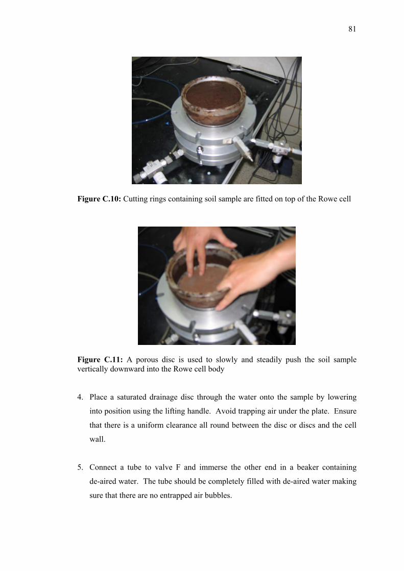
81

Figure C.10: Cutting rings containing soil sample are fitted on top of the Rowe cell

Figure C.11: A porous disc is used to slowly and steadily push the soil sample vertically downward into the Rowe cell body 4. Place a saturated drainage disc through the water onto the sample by lowering

into position using the lifting handle. Avoid trapping air under the plate. Ensure

that there is a uniform clearance all round between the disc or discs and the cell

wall.

5. Connect a tube to valve F and immerse the other end in a beaker containing

de-aired water. The tube should be completely filled with de-aired water making

sure that there are no entrapped air bubbles.

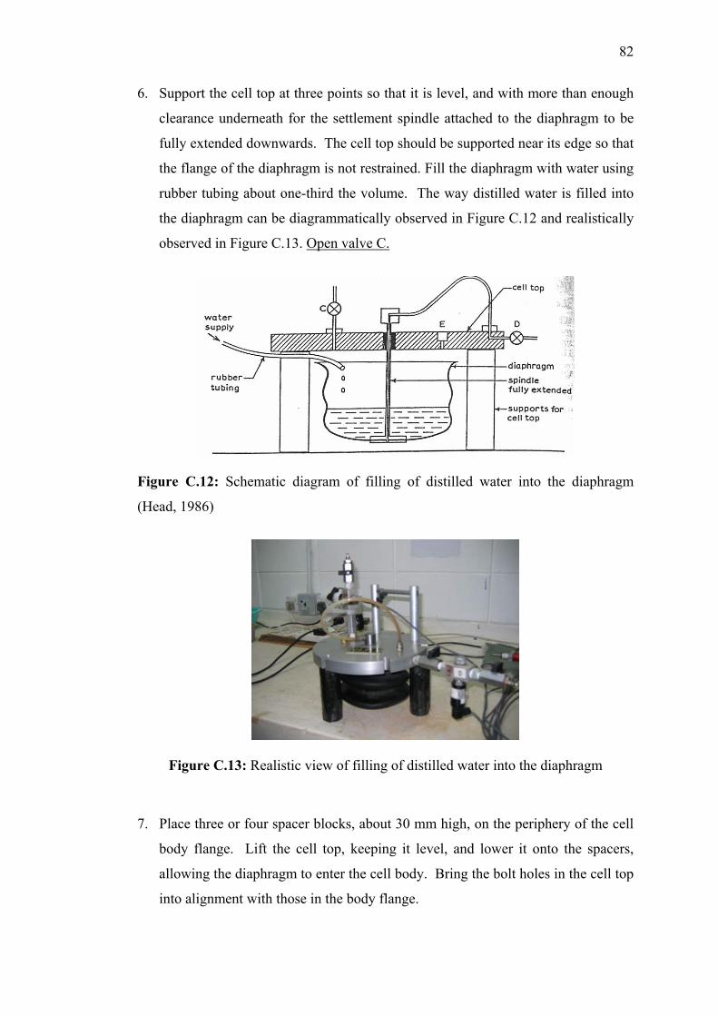
82

6. Support the cell top at three points so that it is level, and with more than enough

clearance underneath for the settlement spindle attached to the diaphragm to be

fully extended downwards. The cell top should be supported near its edge so that

the flange of the diaphragm is not restrained. Fill the diaphragm with water using

rubber tubing about one-third the volume. The way distilled water is filled into

the diaphragm can be diagrammatically observed in Figure C.12 and realistically

observed in Figure C.13. Open valve C.

Figure C.12: Schematic diagram of filling of distilled water into the diaphragm

(Head, 1986)

Figure C.13: Realistic view of filling of distilled water into the diaphragm

7. Place three or four spacer blocks, about 30 mm high, on the periphery of the cell

body flange. Lift the cell top, keeping it level, and lower it onto the spacers,

allowing the diaphragm to enter the cell body. Bring the bolt holes in the cell top

into alignment with those in the body flange.

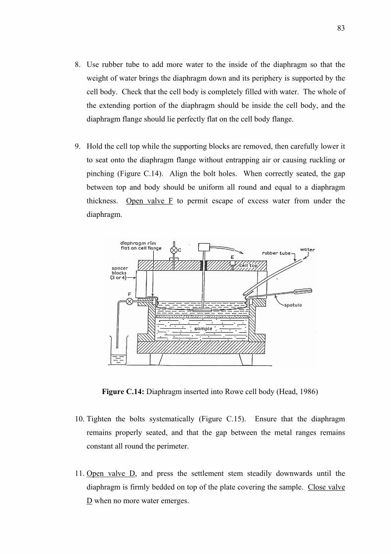
83

8. Use rubber tube to add more water to the inside of the diaphragm so that the

weight of water brings the diaphragm down and its periphery is supported by the

cell body. Check that the cell body is completely filled with water. The whole of

the extending portion of the diaphragm should be inside the cell body, and the

diaphragm flange should lie perfectly flat on the cell body flange.

9. Hold the cell top while the supporting blocks are removed, then carefully lower it

to seat onto the diaphragm flange without entrapping air or causing ruckling or

pinching (Figure C.14). Align the bolt holes. When correctly seated, the gap

between top and body should be uniform all round and equal to a diaphragm

thickness. Open valve F to permit escape of excess water from under the

diaphragm.

Figure C.14: Diaphragm inserted into Rowe cell body (Head, 1986)

10. Tighten the bolts systematically (Figure C.15). Ensure that the diaphragm

remains properly seated, and that the gap between the metal ranges remains

constant all round the perimeter.

11. Open valve D, and press the settlement stem steadily downwards until the

diaphragm is firmly bedded on top of the plate covering the sample. Close valve

D when no more water emerges.

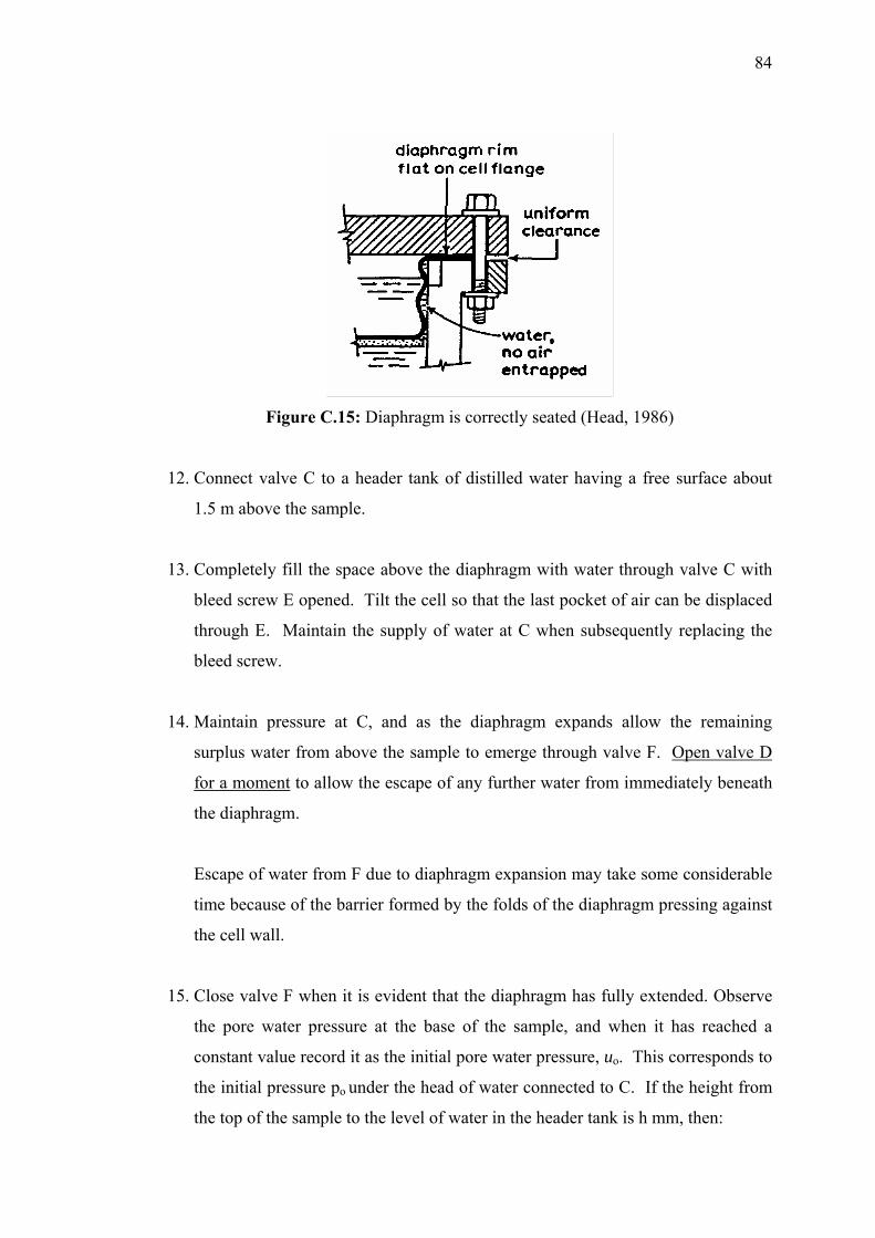
84

Figure C.15: Diaphragm is correctly seated (Head, 1986)

12. Connect valve C to a header tank of distilled water having a free surface about

1.5 m above the sample.

13. Completely fill the space above the diaphragm with water through valve C with

bleed screw E opened. Tilt the cell so that the last pocket of air can be displaced

through E. Maintain the supply of water at C when subsequently replacing the

bleed screw.

14. Maintain pressure at C, and as the diaphragm expands allow the remaining

surplus water from above the sample to emerge through valve F. Open valve D

for a moment to allow the escape of any further water from immediately beneath

the diaphragm.

Escape of water from F due to diaphragm expansion may take some considerable

time because of the barrier formed by the folds of the diaphragm pressing against

the cell wall.

15. Close valve F when it is evident that the diaphragm has fully extended. Observe

the pore water pressure at the base of the sample, and when it has reached a

constant value record it as the initial pore water pressure, uo. This corresponds to

the initial pressure po under the head of water connected to C. If the height from

the top of the sample to the level of water in the header tank is h mm, then:

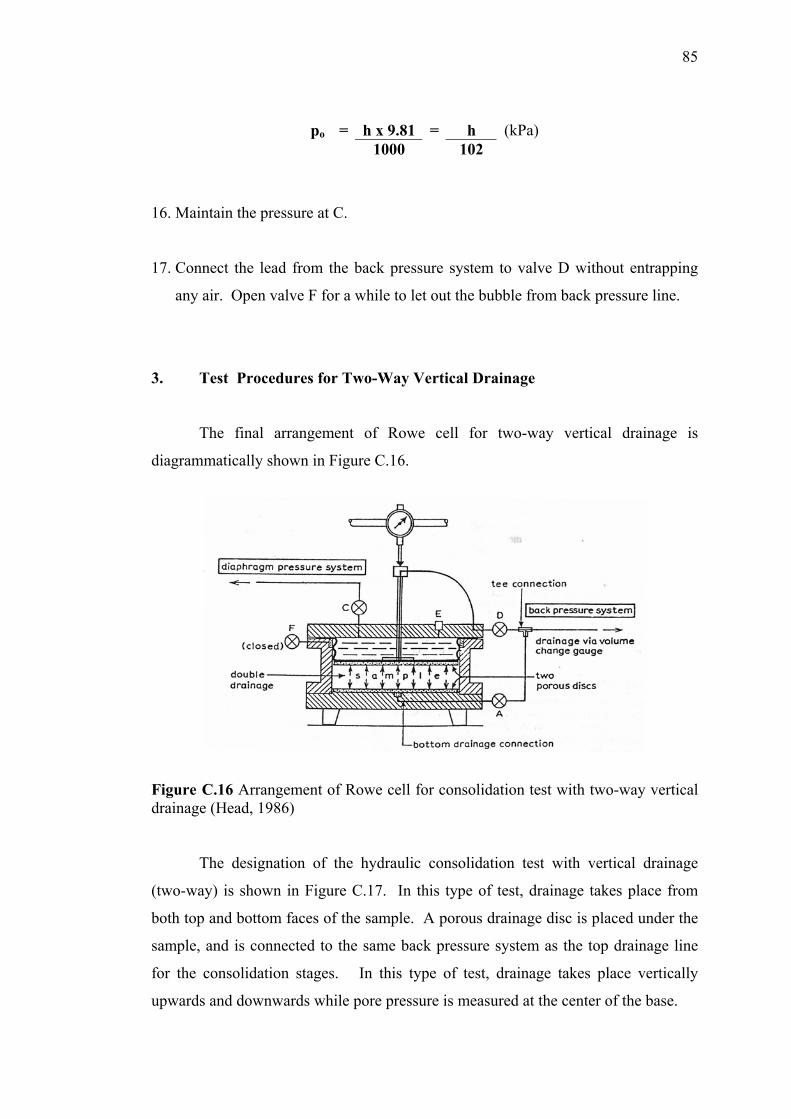
85

po = h x 9.81 = h (kPa) 1000 102

16. Maintain the pressure at C.

17. Connect the lead from the back pressure system to valve D without entrapping

any air. Open valve F for a while to let out the bubble from back pressure line.

3. Test Procedures for Two-Way Vertical Drainage

The final arrangement of Rowe cell for two-way vertical drainage is

diagrammatically shown in Figure C.16.

Figure C.16 Arrangement of Rowe cell for consolidation test with two-way vertical drainage (Head, 1986)

The designation of the hydraulic consolidation test with vertical drainage

(two-way) is shown in Figure C.17. In this type of test, drainage takes place from

both top and bottom faces of the sample. A porous drainage disc is placed under the

sample, and is connected to the same back pressure system as the top drainage line

for the consolidation stages. In this type of test, drainage takes place vertically

upwards and downwards while pore pressure is measured at the center of the base.

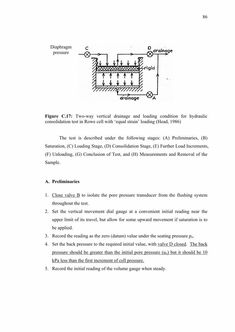
86

Diaphragm pressure

Figure C.17: Two-way vertical drainage and loading condition for hydraulic consolidation test in Rowe cell with ‘equal strain’ loading (Head, 1986)

The test is described under the following stages: (A) Preliminaries, (B)

Saturation, (C) Loading Stage, (D) Consolidation Stage, (E) Further Load Increments,

(F) Unloading, (G) Conclusion of Test, and (H) Measurements and Removal of the

Sample.

A. Preliminaries

1. Close valve B to isolate the pore pressure transducer from the flushing system

throughout the test.

2. Set the vertical movement dial gauge at a convenient initial reading near the

upper limit of its travel, but allow for some upward movement if saturation is to

be applied.

3. Record the reading as the zero (datum) value under the seating pressure po.

4. Set the back pressure to the required initial value, with valve D closed. The back

pressure should be greater than the initial pore pressure (uo) but it should be 10

kPa less than the first increment of cell pressure.

5. Record the initial reading of the volume gauge when steady.

87

B. Saturation

Saturation by the application of increments of back pressure is desirable for

undisturbed samples taken from above water table. For this type of test, application

of 10 kPa back pressure is used.

Saturation is generally accepted as being complete when the value of the pore

pressure parameter B reaches about 0.96.

C. Loading Stage

1. With the drainage lines valve A and valve D closed and valve C open, increase

the diaphragm pressure steadily to the first increment. Open valve A valve D

when set.

First increment of diaphragm pressure is taken as 50 kPa for this type of test.

2. Open valve F to allow excess water to escape from behind the diaphragm for a

short time just to allow excess water from the top of the sample.

3. Wait until the pore pressure reaches a steady value equal to diaphragm pressure.

If the sample is virtually saturated the increase in pore pressure should almost

equal the pressure increment applied to the sample.

4. Record any settlement indicated by the dial gauge before starting consolidation.

D. Consolidation Stage

Consolidation is started by opening the drainage outlets (valve A and valve D in

Figure C.9) and at the same instant starting the clock. Read the following data:

a. Vertical settlement

b. Pore water pressure

c. Volume change on back pressure line

d. Diaphragm pressure (check)

The primary consolidation phase is completed when the pore pressure has fallen to

the value of the back pressure. Wait for secondary consolidation to take place.

88

E. Further Load Increments

1. Increase the diaphragm pressure to give the next value of effective stress. Allow

excess water to drain from behind the diaphragm (valve F) if necessary.

2. The pore pressure should then be allowed to reach equilibrium before

proceedings to the next consolidation stage.

3. Repeat the above steps for 100 kPa and 200 kPa consolidation pressures.

F. Unloading

Unloading is needed for evaluation of the effect of surcharge on the compressibility

characteristics of peat. In this case, the sample was loaded to the pre-consolidation

pressure (estimated based on oedometer test data, 30 kPa) and loaded to 100 kPa. At

the end of consolidation test under 100 kPa, the soil was unloaded back to 30 kPa.

For unloading stage, diaphragm pressure is reduced with valve D closed. It should

be followed by swelling stage with valve D open, during which upward movement,

volume increase and pore-pressure readings are taken in the same way as

consolidation process. The pore-pressure should be allowed to reach equilibrium at

the end of each stage before proceeding to the next stage of loading. The following

stage of loading in this case is 100 kPa and 150 kPa.

G. Conclusion of Test

1. Reduce the pressure to the initial seating pressure, po

2. When equilibrium has been achieved, record the final settlement, volume change

and pore pressure readings.

3. Close valve A and open valves C, D and F, allowing surplus water to escape.

Unbolt and remove the cell top and place it on the bench supports.

H. Measurement and Removal of Sample

1. Remove the porous disc to expose the sample surface. Measure the diameter and

height of the sample.

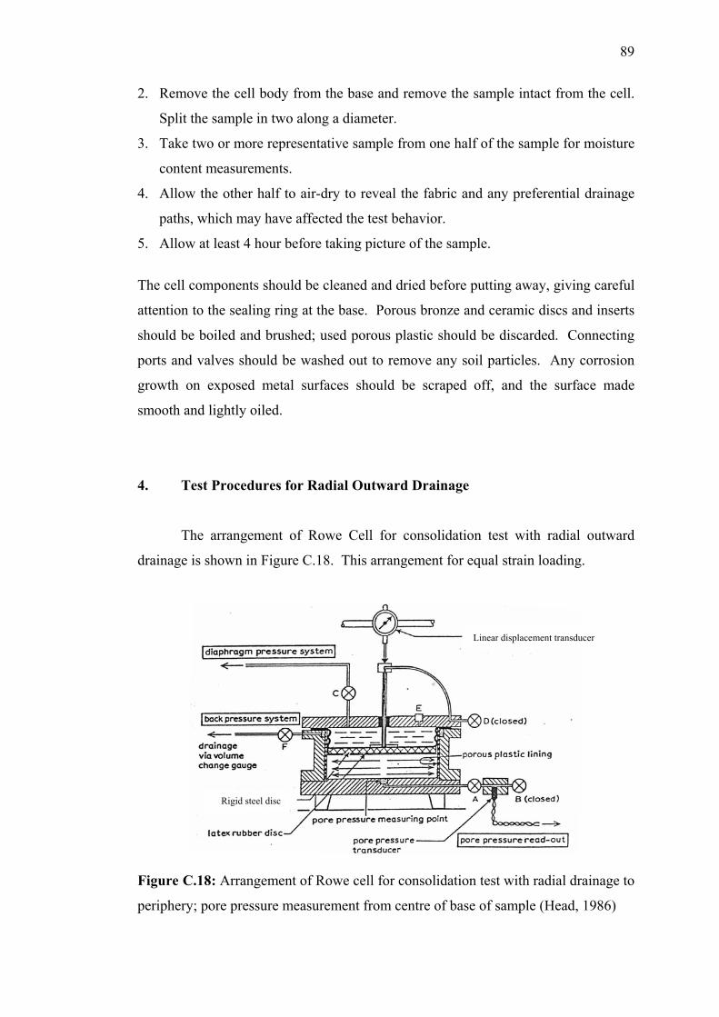
89

2. Remove the cell body from the base and remove the sample intact from the cell.

Split the sample in two along a diameter.

3. Take two or more representative sample from one half of the sample for moisture

content measurements.

4. Allow the other half to air-dry to reveal the fabric and any preferential drainage

paths, which may have affected the test behavior.

5. Allow at least 4 hour before taking picture of the sample.

The cell components should be cleaned and dried before putting away, giving careful

attention to the sealing ring at the base. Porous bronze and ceramic discs and inserts

should be boiled and brushed; used porous plastic should be discarded. Connecting

ports and valves should be washed out to remove any soil particles. Any corrosion

growth on exposed metal surfaces should be scraped off, and the surface made

smooth and lightly oiled.

4. Test Procedures for Radial Outward Drainage

The arrangement of Rowe Cell for consolidation test with radial outward

drainage is shown in Figure C.18. This arrangement for equal strain loading.

Linear displacement transducer

Rigid steel disc

Figure C.18: Arrangement of Rowe cell for consolidation test with radial drainage to

periphery; pore pressure measurement from centre of base of sample (Head, 1986)

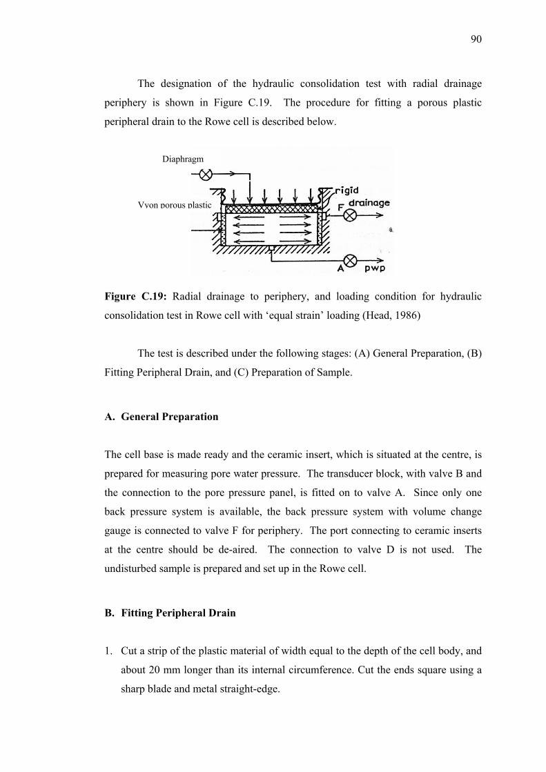
90

The designation of the hydraulic consolidation test with radial drainage

periphery is shown in Figure C.19. The procedure for fitting a porous plastic

peripheral drain to the Rowe cell is described below.

Diaphragm

Vyon porous plastic

Figure C.19: Radial drainage to periphery, and loading condition for hydraulic

consolidation test in Rowe cell with ‘equal strain’ loading (Head, 1986)

The test is described under the following stages: (A) General Preparation, (B)

Fitting Peripheral Drain, and (C) Preparation of Sample.

A. General Preparation

The cell base is made ready and the ceramic insert, which is situated at the centre, is

prepared for measuring pore water pressure. The transducer block, with valve B and

the connection to the pore pressure panel, is fitted on to valve A. Since only one

back pressure system is available, the back pressure system with volume change

gauge is connected to valve F for periphery. The port connecting to ceramic inserts

at the centre should be de-aired. The connection to valve D is not used. The

undisturbed sample is prepared and set up in the Rowe cell.

B. Fitting Peripheral Drain

1. Cut a strip of the plastic material of width equal to the depth of the cell body, and

about 20 mm longer than its internal circumference. Cut the ends square using a

sharp blade and metal straight-edge.

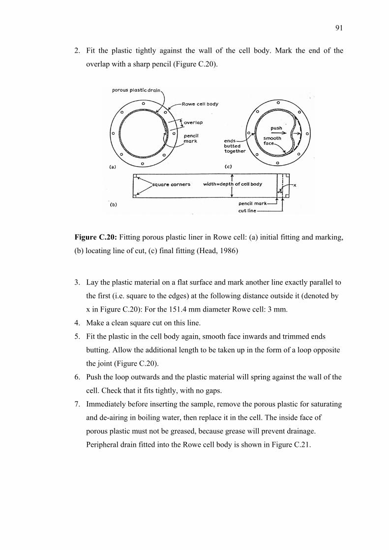
91

2. Fit the plastic tightly against the wall of the cell body. Mark the end of the

overlap with a sharp pencil (Figure C.20).

Figure C.20: Fitting porous plastic liner in Rowe cell: (a) initial fitting and marking,

(b) locating line of cut, (c) final fitting (Head, 1986)

3. Lay the plastic material on a flat surface and mark another line exactly parallel to

the first (i.e. square to the edges) at the following distance outside it (denoted by

x in Figure C.20): For the 151.4 mm diameter Rowe cell: 3 mm.

4. Make a clean square cut on this line.

5. Fit the plastic in the cell body again, smooth face inwards and trimmed ends

butting. Allow the additional length to be taken up in the form of a loop opposite

the joint (Figure C.20).

6. Push the loop outwards and the plastic material will spring against the wall of the

cell. Check that it fits tightly, with no gaps.

7. Immediately before inserting the sample, remove the porous plastic for saturating

and de-airing in boiling water, then replace it in the cell. The inside face of

porous plastic must not be greased, because grease will prevent drainage.

Peripheral drain fitted into the Rowe cell body is shown in Figure C.21.

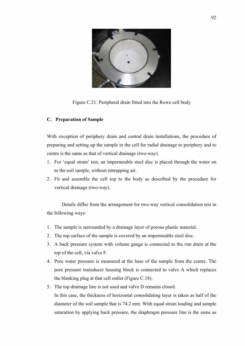
92

Figure C.21: Peripheral drain fitted into the Rowe cell body

C. Preparation of Sample

With exception of periphery drain and central drain installations, the procedure of

preparing and setting up the sample in the cell for radial drainage to periphery and to

centre is the same as that of vertical drainage (two-way).

1. For ‘equal strain’ test, an impermeable steel disc is placed through the water on

to the soil sample, without entrapping air.

2. Fit and assemble the cell top to the body as described by the procedure for

vertical drainage (two-way).

Details differ from the arrangement for two-way vertical consolidation test in

the following ways:

1. The sample is surrounded by a drainage layer of porous plastic material.

2. The top surface of the sample is covered by an impermeable steel disc.

3. A back pressure system with volume gauge is connected to the rim drain at the

top of the cell, via valve F.

4. Pore water pressure is measured at the base of the sample from the centre. The

pore pressure transducer housing block is connected to valve A which replaces

the blanking plug at that cell outlet (Figure C.18).

5. The top drainage line is not used and valve D remains closed.

In this case, the thickness of horizontal consolidating layer is taken as half of the

diameter of the soil sample that is 74.2 mm. With equal strain loading and sample

saturation by applying back pressure, the diaphragm pressure line is the same as

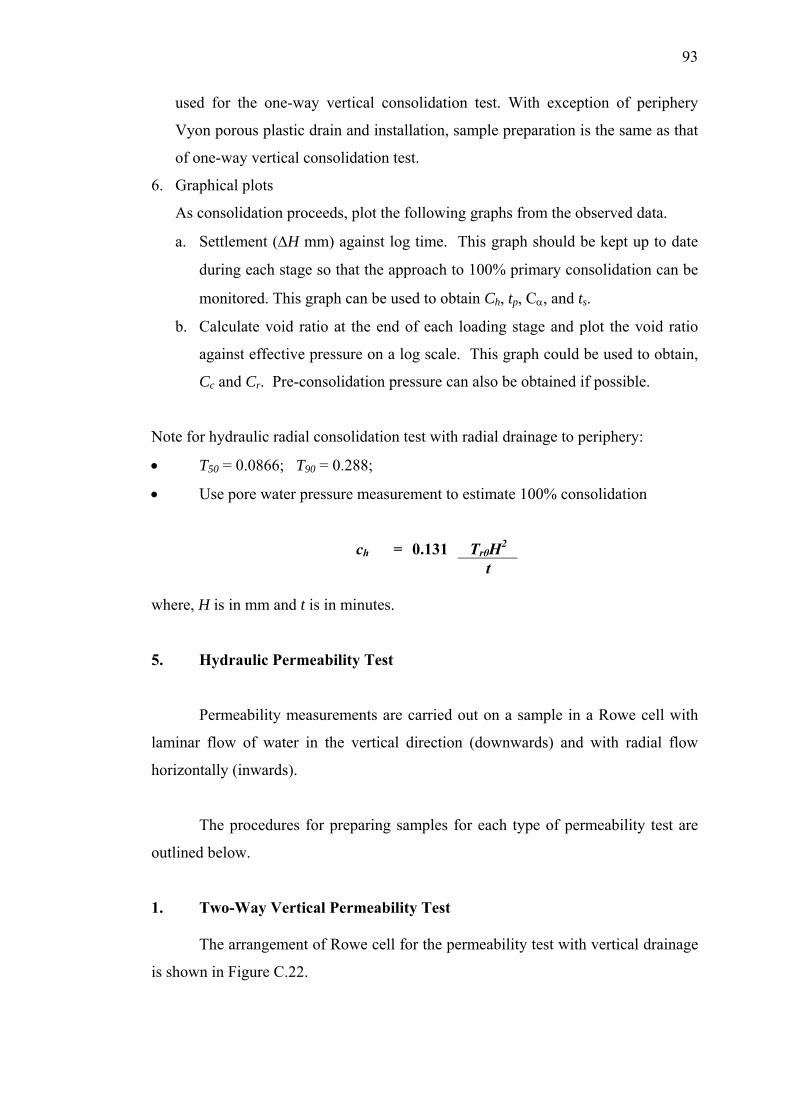
93

used for the one-way vertical consolidation test. With exception of periphery

Vyon porous plastic drain and installation, sample preparation is the same as that

of one-way vertical consolidation test.

6. Graphical plots

As consolidation proceeds, plot the following graphs from the observed data.

a. Settlement (∆H mm) against log time. This graph should be kept up to date

during each stage so that the approach to 100% primary consolidation can be

monitored. This graph can be used to obtain Ch, tp, Cα, and ts.

b. Calculate void ratio at the end of each loading stage and plot the void ratio

against effective pressure on a log scale. This graph could be used to obtain,

Cc and Cr. Pre-consolidation pressure can also be obtained if possible.

Note for hydraulic radial consolidation test with radial drainage to periphery:

• T50 = 0.0866; T90 = 0.288;

• Use pore water pressure measurement to estimate 100% consolidation

ch = 0.131 TrθH2

t

where, H is in mm and t is in minutes.

5. Hydraulic Permeability Test

Permeability measurements are carried out on a sample in a Rowe cell with

laminar flow of water in the vertical direction (downwards) and with radial flow

horizontally (inwards).

The procedures for preparing samples for each type of permeability test are

outlined below.

1. Two-Way Vertical Permeability Test

The arrangement of Rowe cell for the permeability test with vertical drainage

is shown in Figure C.22.

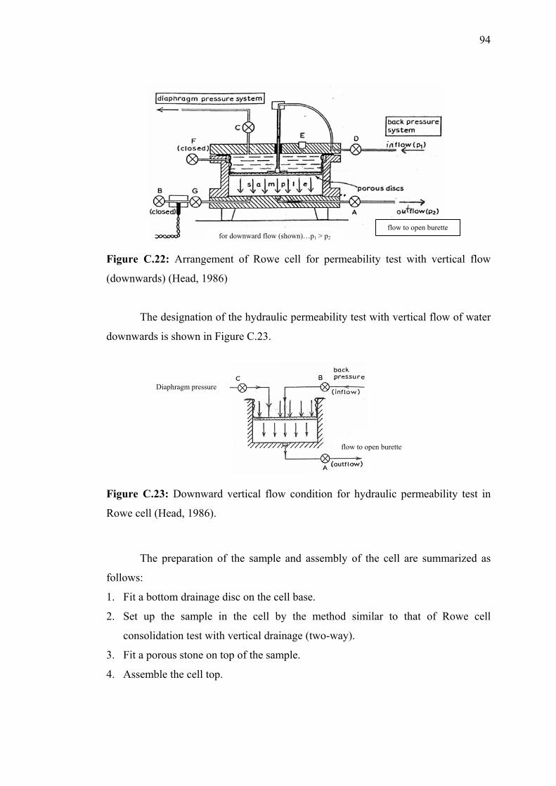
94

flow to open burette

for downward flow (shown)…p1 > p2

Figure C.22: Arrangement of Rowe cell for permeability test with vertical flow

(downwards) (Head, 1986)

The designation of the hydraulic permeability test with vertical flow of water

downwards is shown in Figure C.23.

Diaphragm pressure

flow to open burette

Figure C.23: Downward vertical flow condition for hydraulic permeability test in

Rowe cell (Head, 1986).

The preparation of the sample and assembly of the cell are summarized as

follows:

1. Fit a bottom drainage disc on the cell base.

2. Set up the sample in the cell by the method similar to that of Rowe cell

consolidation test with vertical drainage (two-way).

3. Fit a porous stone on top of the sample.

4. Assemble the cell top.

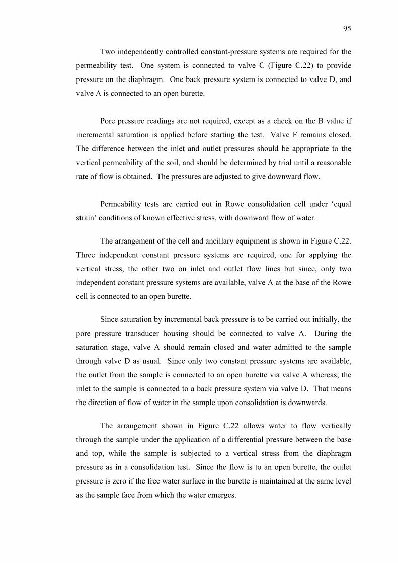
95

Two independently controlled constant-pressure systems are required for the

permeability test. One system is connected to valve C (Figure C.22) to provide

pressure on the diaphragm. One back pressure system is connected to valve D, and

valve A is connected to an open burette.

Pore pressure readings are not required, except as a check on the B value if

incremental saturation is applied before starting the test. Valve F remains closed.

The difference between the inlet and outlet pressures should be appropriate to the

vertical permeability of the soil, and should be determined by trial until a reasonable

rate of flow is obtained. The pressures are adjusted to give downward flow.

Permeability tests are carried out in Rowe consolidation cell under ‘equal

strain’ conditions of known effective stress, with downward flow of water.

The arrangement of the cell and ancillary equipment is shown in Figure C.22.

Three independent constant pressure systems are required, one for applying the

vertical stress, the other two on inlet and outlet flow lines but since, only two

independent constant pressure systems are available, valve A at the base of the Rowe

cell is connected to an open burette.

Since saturation by incremental back pressure is to be carried out initially, the

pore pressure transducer housing should be connected to valve A. During the

saturation stage, valve A should remain closed and water admitted to the sample

through valve D as usual. Since only two constant pressure systems are available,

the outlet from the sample is connected to an open burette via valve A whereas; the

inlet to the sample is connected to a back pressure system via valve D. That means

the direction of flow of water in the sample upon consolidation is downwards.

The arrangement shown in Figure C.22 allows water to flow vertically

through the sample under the application of a differential pressure between the base

and top, while the sample is subjected to a vertical stress from the diaphragm

pressure as in a consolidation test. Since the flow is to an open burette, the outlet

pressure is zero if the free water surface in the burette is maintained at the same level

as the sample face from which the water emerges.

96

The sample is first consolidated to the required effective stress by the

application of diaphragm loading. Consolidation should be virtually completed, i.e.

the excess pore pressure should be at least 95% dissipated before starting a

permeability test.

The procedure for two-way vertical permeability test using Rowe cell is as follows: 1. The test is first carried out by adjusting the pressure difference across the sample

to provide a reasonable rate of flow through it. The hydraulic gradient required

to induce flow should be ascertained by trial, starting with equal pressures on the

inlet and outlet lines and progressively increasing the inlet pressure, which must

never exceed the diaphragm pressure. Since only one back pressure system is

used, the outlet drainage is connected to an open burette as shown in Figure C.12.

Figure C.24: Arrangement for hydraulic vertical permeability test using one back

pressure system for downward flow (Head, 1986)

2. When a steady rate of flow has been established, measure the time required for a

given volume to pass through. The volume of water is measured from an open

burette incorporated in the outlet of the soil sample via valve A.

3. Calculate the cumulative flow, Q (ml) up to the time of each reading, and plot a

graph of Q against time, t (minutes), as the test proceeds. Continue the test until

it can be seen that a steady rate of flow is reached, i.e. the graph is linear.

4. From the linear part of the graph, measure the slope to calculate the rate of flow,

q (ml/minute); i.e. q = δQ / δt (ml/minute).

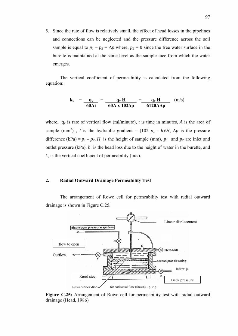
97

5. Since the rate of flow is relatively small, the effect of head losses in the pipelines

and connections can be neglected and the pressure difference across the soil

sample is equal to p1 – p2 = ∆p where, p2 = 0 since the free water surface in the

burette is maintained at the same level as the sample face from which the water

emerges.

The vertical coefficient of permeability is calculated from the following

equation:

kv = qv = qv H = qv H (m/s) 60Ai 60A x 102∆p 6120A∆p

where, qv is rate of vertical flow (ml/minute), t is time in minutes, A is the area of

sample (mm2) , I is the hydraulic gradient = (102 p1 - h)/H, ∆p is the pressure

difference (kPa) = p1 – p2, H is the height of sample (mm), p1 and p2 are inlet and

outlet pressure (kPa), h is the head loss due to the height of water in the burette, and

kv is the vertical coefficient of permeability (m/s).

2. Radial Outward Drainage Permeability Test

The arrangement of Rowe cell for permeability test with radial outward

drainage is shown in Figure C.25.

Linear displacement

flow to open

Outflow,

Inflow, p1

Rigid steel Back pressure

for horizontal flow (shown)…p1 > p2

Figure C.25: Arrangement of Rowe cell for permeability test with radial outward drainage (Head, 1986)

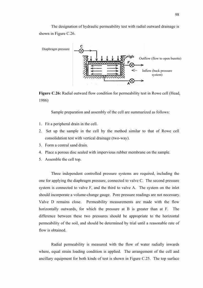
98

The designation of hydraulic permeability test with radial outward drainage is

shown in Figure C.26.

Diaphragm pressure

Outflow (flow to open burette)

Inflow (back pressure system)

Figure C.26: Radial outward flow condition for permeability test in Rowe cell (Head,

1986)

Sample preparation and assembly of the cell are summarized as follows:

1. Fit a peripheral drain in the cell.

2. Set up the sample in the cell by the method similar to that of Rowe cell

consolidation test with vertical drainage (two-way).

3. Form a central sand drain.

4. Place a porous disc sealed with impervious rubber membrane on the sample.

5. Assemble the cell top.

Three independent controlled pressure systems are required, including the

one for applying the diaphragm pressure, connected to valve C. The second pressure

system is connected to valve F, and the third to valve A. The system on the inlet

should incorporate a volume-change gauge. Pore pressure readings are not necessary.

Valve D remains close. Permeability measurements are made with the flow

horizontally outwards, for which the pressure at B is greater than at F. The

difference between these two pressures should be appropriate to the horizontal

permeability of the soil, and should be determined by trial until a reasonable rate of

flow is obtained.

Radial permeability is measured with the flow of water radially inwards

where, equal strain loading condition is applied. The arrangement of the cell and

ancillary equipment for both kinds of test is shown in Figure C.25. The top surface

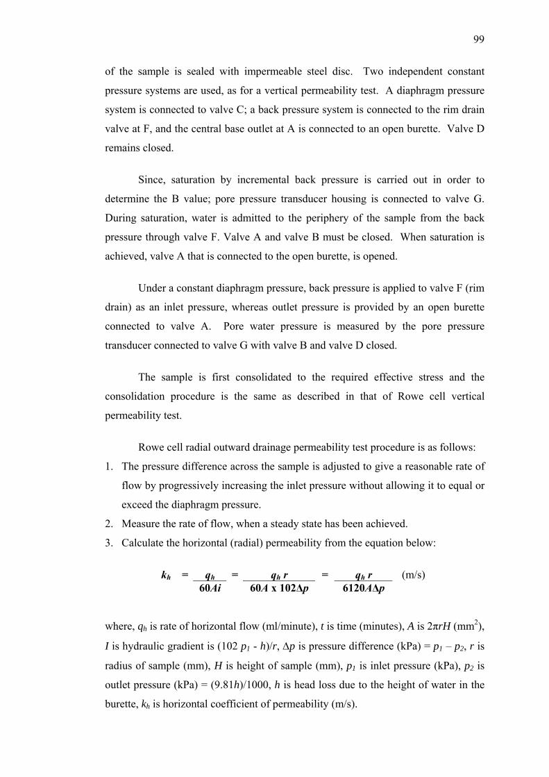
99

of the sample is sealed with impermeable steel disc. Two independent constant

pressure systems are used, as for a vertical permeability test. A diaphragm pressure

system is connected to valve C; a back pressure system is connected to the rim drain

valve at F, and the central base outlet at A is connected to an open burette. Valve D

remains closed.

Since, saturation by incremental back pressure is carried out in order to

determine the B value; pore pressure transducer housing is connected to valve G.

During saturation, water is admitted to the periphery of the sample from the back

pressure through valve F. Valve A and valve B must be closed. When saturation is

achieved, valve A that is connected to the open burette, is opened.

Under a constant diaphragm pressure, back pressure is applied to valve F (rim

drain) as an inlet pressure, whereas outlet pressure is provided by an open burette

connected to valve A. Pore water pressure is measured by the pore pressure

transducer connected to valve G with valve B and valve D closed.

The sample is first consolidated to the required effective stress and the

consolidation procedure is the same as described in that of Rowe cell vertical

permeability test.

Rowe cell radial outward drainage permeability test procedure is as follows:

1. The pressure difference across the sample is adjusted to give a reasonable rate of

flow by progressively increasing the inlet pressure without allowing it to equal or

exceed the diaphragm pressure.

2. Measure the rate of flow, when a steady state has been achieved.

3. Calculate the horizontal (radial) permeability from the equation below:

kh = qh = qh r = qh r (m/s) 60Ai 60A x 102∆p 6120A∆p

where, qh is rate of horizontal flow (ml/minute), t is time (minutes), A is 2πrH (mm2),

I is hydraulic gradient is (102 p1 - h)/r, ∆p is pressure difference (kPa) = p1 – p2, r is

radius of sample (mm), H is height of sample (mm), p1 is inlet pressure (kPa), p2 is

outlet pressure (kPa) = (9.81h)/1000, h is head loss due to the height of water in the

burette, kh is horizontal coefficient of permeability (m/s).

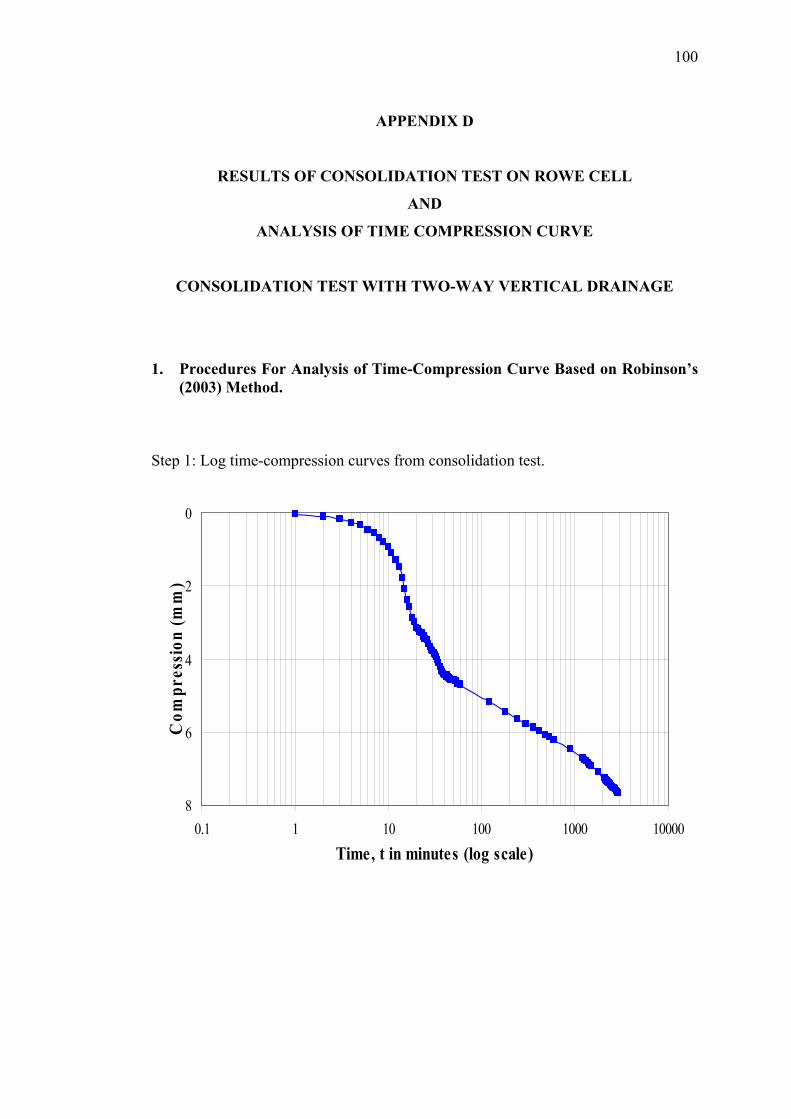
100

APPENDIX D

RESULTS OF CONSOLIDATION TEST ON ROWE CELL

AND

ANALYSIS OF TIME COMPRESSION CURVE

CONSOLIDATION TEST WITH TWO-WAY VERTICAL DRAINAGE

1. Procedures For Analysis of Time-Compression Curve Based on Robinson’s

(2003) Method. Step 1: Log time-compression curves from consolidation test.

0

2

4

6

80.1 1 10 100 1000 10000

Time, t in minutes (log scale)

Com

pres

sion

(mm

)

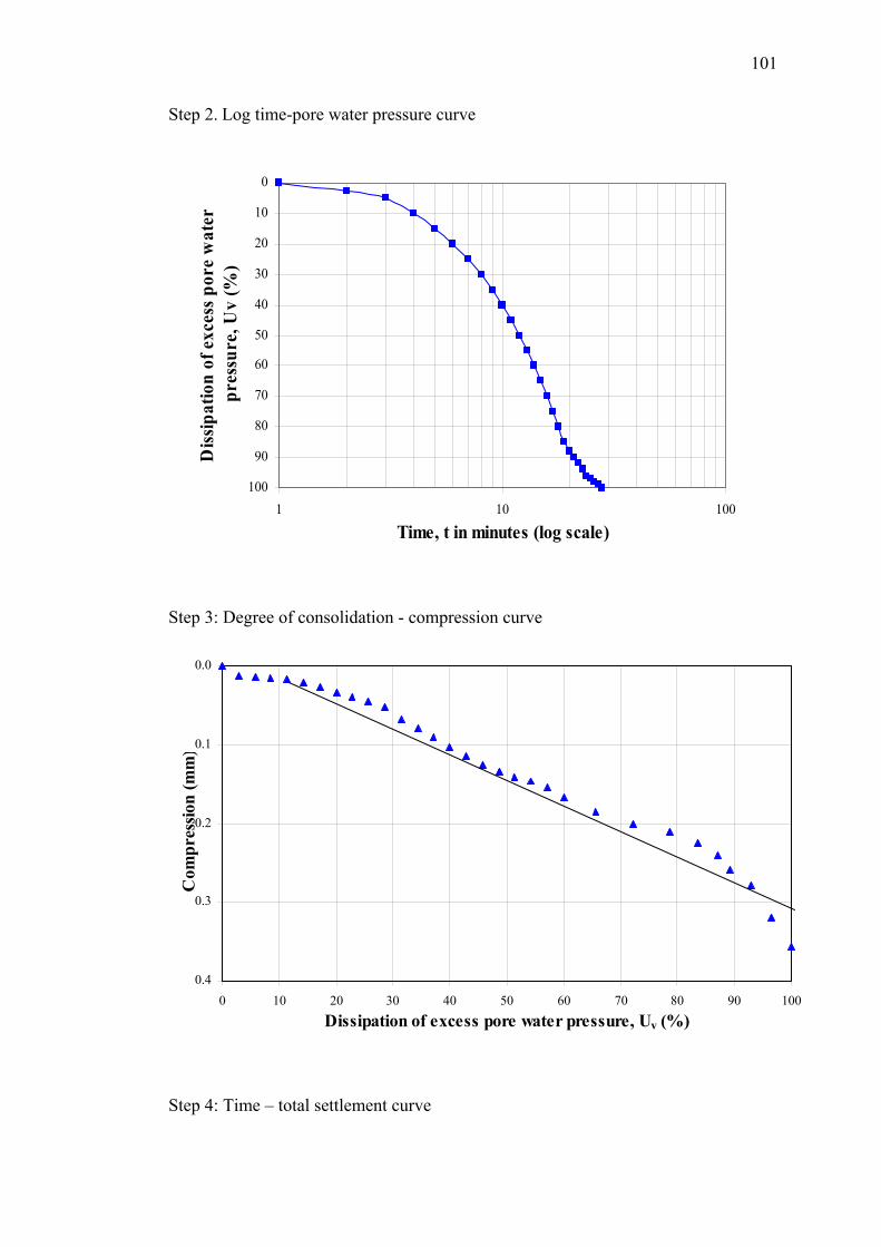
101

Step 2. Log time-pore water pressure curve

0

10

20

30

40

50

60

70

80

90

1001 10 100

Time, t in minutes (log scale)

Diss

ipat

ion

of e

xces

s por

e w

ater

pr

essu

re, U

v (%

)

Step 3: Degree of consolidation - compression curve

0.0

0.1

0.2

0.3

0.40 10 20 30 40 50 60 70 80 90 1

Dissipation of excess pore water pressure, Uv (%)

Com

pres

sion

(mm

00

)

Step 4: Time – total settlement curve

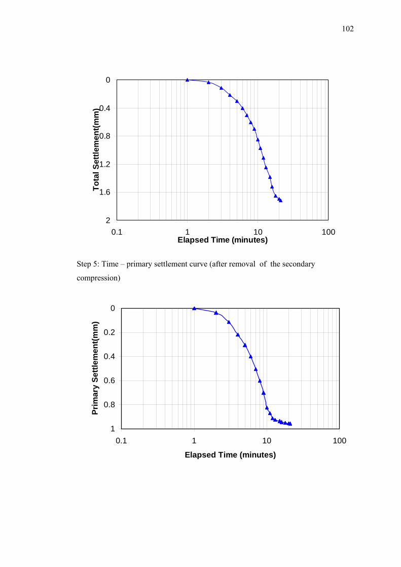
102

0

0.4

0.8

1.2

1.6

20.1 1 10 100

Elapsed Time (minutes)

Tota

l Set

tlem

ent(m

m)

Step 5: Time – primary settlement curve (after removal of the secondary

compression)

0

0.2

0.4

0.6

0.8

10.1 1 10 100

Elapsed Time (minutes)

Prim

ary

Settl

emen

t(mm

)

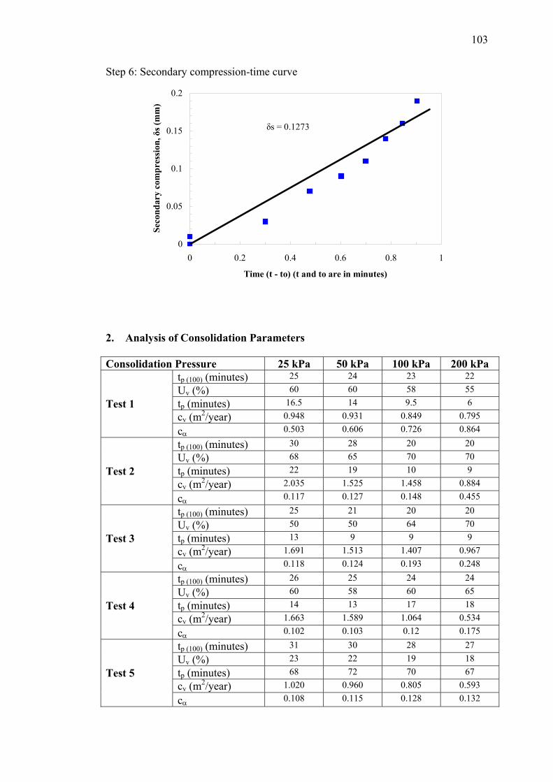
103

Step 6: Secondary compression-time curve

δs = 0.1273

0

0.05

0.1

0.15

0.2

0 0.2 0.4 0.6 0.8 1

Time (t - to) (t and to are in minutes)

Seco

ndar

y co

mpr

essi

on, δ

s (m

m)

2. Analysis of Consolidation Parameters Consolidation Pressure 25 kPa 50 kPa 100 kPa 200 kPa

tp (100) (minutes) 25 24 23 22 Uv (%) 60 60 58 55 tp (minutes) 16.5 14 9.5 6 cv (m2/year) 0.948 0.931 0.849 0.795

Test 1

cα 0.503 0.606 0.726 0.864

tp (100) (minutes) 30 28 20 20 Uv (%) 68 65 70 70 tp (minutes) 22 19 10 9 cv (m2/year) 2.035 1.525 1.458 0.884

Test 2

cα 0.117 0.127 0.148 0.455

tp (100) (minutes) 25 21 20 20 Uv (%) 50 50 64 70 tp (minutes) 13 9 9 9 cv (m2/year) 1.691 1.513 1.407 0.967

Test 3

cα 0.118 0.124 0.193 0.248

tp (100) (minutes) 26 25 24 24 Uv (%) 60 58 60 65 tp (minutes) 14 13 17 18 cv (m2/year) 1.663 1.589 1.064 0.534

Test 4

cα 0.102 0.103 0.12 0.175

tp (100) (minutes) 31 30 28 27 Uv (%) 23 22 19 18 tp (minutes) 68 72 70 67 cv (m2/year) 1.020 0.960 0.805 0.593

Test 5

cα 0.108 0.115 0.128 0.132

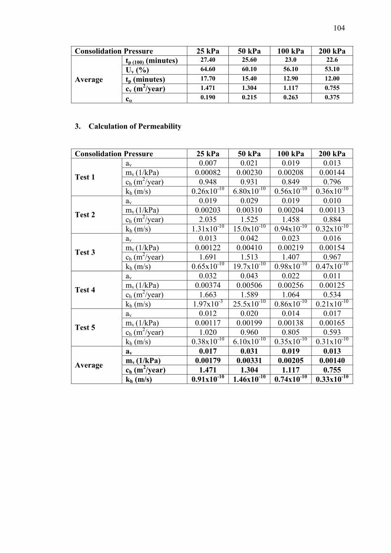
104

Consolidation Pressure 25 kPa 50 kPa 100 kPa 200 kPa tp (100) (minutes) 27.40 25.60 23.0 22.6 Uv (%) 64.60 60.10 56.10 53.10 tp (minutes) 17.70 15.40 12.90 12.00 cv (m2/year) 1.471 1.304 1.117 0.755

Average

cα 0.190 0.215 0.263 0.375

3. Calculation of Permeability Consolidation Pressure 25 kPa 50 kPa 100 kPa 200 kPa

av 0.007 0.021 0.019 0.013 mv (1/kPa) 0.00082 0.00230 0.00208 0.00144 ch (m2/year) 0.948 0.931 0.849 0.796 Test 1

kh (m/s) 0.26x10-10 6.80x10-10 0.56x10-10 0.36x10-10

av 0.019 0.029 0.019 0.010 mv (1/kPa) 0.00203 0.00310 0.00204 0.00113 ch (m2/year) 2.035 1.525 1.458 0.884 Test 2

kh (m/s) 1.31x10-10 15.0x10-10 0.94x10-10 0.32x10-10

av 0.013 0.042 0.023 0.016 mv (1/kPa) 0.00122 0.00410 0.00219 0.00154 ch (m2/year) 1.691 1.513 1.407 0.967 Test 3

kh (m/s) 0.65x10-10 19.7x10-10 0.98x10-10 0.47x10-10

av 0.032 0.043 0.022 0.011 mv (1/kPa) 0.00374 0.00506 0.00256 0.00125 ch (m2/year) 1.663 1.589 1.064 0.534 Test 4

kh (m/s) 1.97x10-3 25.5x10-10 0.86x10-10 0.21x10-10

av 0.012 0.020 0.014 0.017 mv (1/kPa) 0.00117 0.00199 0.00138 0.00165 ch (m2/year) 1.020 0.960 0.805 0.593 Test 5

kh (m/s) 0.38x10-10 6.10x10-10 0.35x10-10 0.31x10-10

av 0.017 0.031 0.019 0.013 mv (1/kPa) 0.00179 0.00331 0.00205 0.00140 ch (m2/year) 1.471 1.304 1.117 0.755 Average

kh (m/s) 0.91x10-10 1.46x10-10 0.74x10-10 0.33x10-10

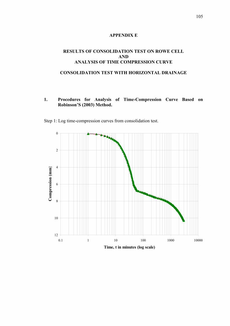
105

APPENDIX E

RESULTS OF CONSOLIDATION TEST ON ROWE CELL AND

ANALYSIS OF TIME COMPRESSION CURVE

CONSOLIDATION TEST WITH HORIZONTAL DRAINAGE

1. Procedures for Analysis of Time-Compression Curve Based on

Robinson’S (2003) Method. Step 1: Log time-compression curves from consolidation test.

0

2

4

6

8

10

120.1 1 10 100 1000 10000

Time, t in minutes (log scale)

Com

pres

sion

(mm

)

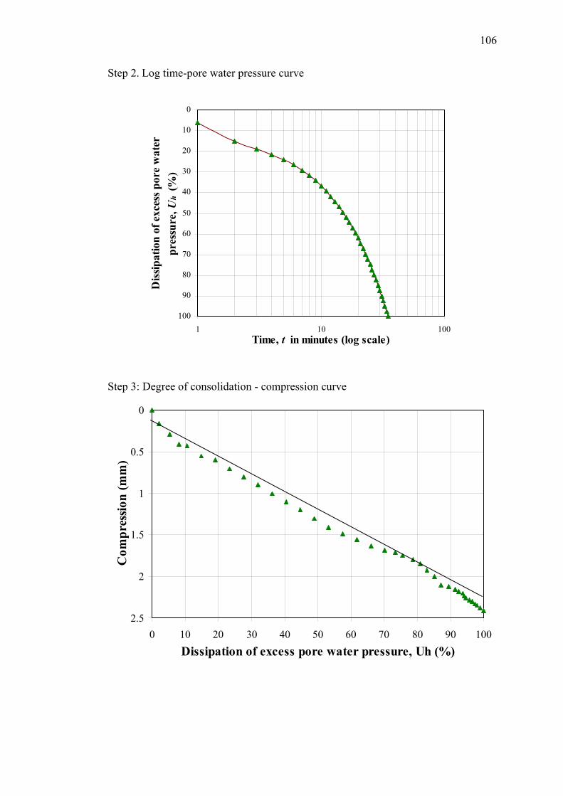
106

Step 2. Log time-pore water pressure curve

0

10

20

30

40

50

60

70

80

90

1001 10 100

Time, t in minutes (log scale)

Diss

ipat

ion

of e

xces

s por

e w

ater

pres

sure

, Uh

(%)

Step 3: Degree of consolidation - compression curve

0

0.5

1

1.5

2

2.50 10 20 30 40 50 60 70 80 90 10

Dissipation of excess pore water pressure, Uh (%)

Com

pres

sion

(mm

)

0

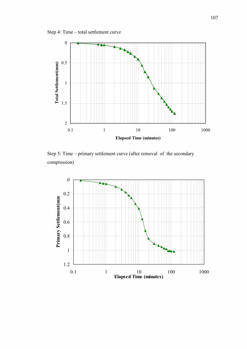
107

Step 4: Time – total settlement curve

0

0.5

1

1.5

20.1 1 10 100 1000

Elapsed Time (minutes)

Tot

al S

ettle

men

t(m

m)

Step 5: Time – primary settlement curve (after removal of the secondary

compression)

0

0.2

0.4

0.6

0.8

1

1.20.1 1 10 100 1000

Elapsed Time (minutes)

Prim

ary

Sett

lem

ent(

mm

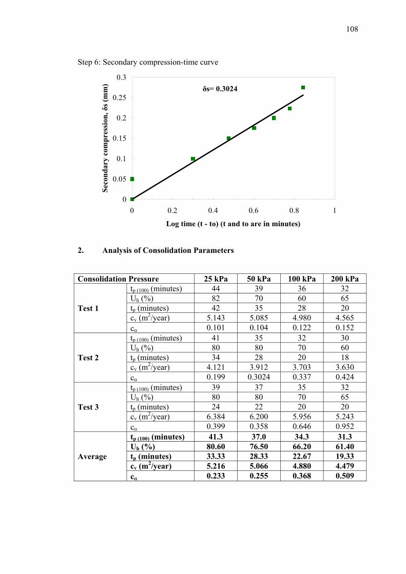
108

Step 6: Secondary compression-time curve

δs= 0.3024

0

0.05

0.1

0.15

0.2

0.25

0.3

0 0.2 0.4 0.6 0.8 1

Log time (t - to) (t and to are in minutes)

Seco

ndar

y co

mpr

essi

on, δ

s (m

m)

2. Analysis of Consolidation Parameters

Consolidation Pressure 25 kPa 50 kPa 100 kPa 200 kPa tp (100) (minutes) 44 39 36 32 Uh (%) 82 70 60 65 tp (minutes) 42 35 28 20 cv (m2/year) 5.143 5.085 4.980 4.565

Test 1

cα 0.101 0.104 0.122 0.152 tp (100) (minutes) 41 35 32 30 Uh (%) 80 80 70 60 tp (minutes) 34 28 20 18 cv (m2/year) 4.121 3.912 3.703 3.630

Test 2

cα 0.199 0.3024 0.337 0.424 tp (100) (minutes) 39 37 35 32 Uh (%) 80 80 70 65 tp (minutes) 24 22 20 20 cv (m2/year) 6.384 6.200 5.956 5.243

Test 3

cα 0.399 0.358 0.646 0.952 tp (100) (minutes) 41.3 37.0 34.3 31.3 Uh (%) 80.60 76.50 66.20 61.40 tp (minutes) 33.33 28.33 22.67 19.33 cv (m2/year) 5.216 5.066 4.880 4.479

Average

cα 0.233 0.255 0.368 0.509

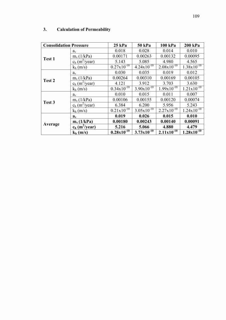
109

3. Calculation of Permeability

Consolidation Pressure 25 kPa 50 kPa 100 kPa 200 kPa av 0.018 0.028 0.014 0.010 mv (1/kPa) 0.00171 0.00263 0.00132 0.00095 ch (m2/year) 5.143 5.085 4.980 4.565 Test 1

kh (m/s) 0.27x10-10 4.24x10-10 2.08x10-10 1.38x10-10

av 0.030 0.035 0.019 0.012 mv (1/kPa) 0.00264 0.00310 0.00169 0.00105 ch (m2/year) 4.121 3.912 3.703 3.630 Test 2

kh (m/s) 0.34x10-10 3.90x10-10 1.99x10-10 1.21x10-10

av 0.010 0.015 0.011 0.007 mv (1/kPa) 0.00106 0.00155 0.00120 0.00074 ch (m2/year) 6.384 6.200 5.956 5.243 Test 3

kh (m/s) 0.21x10-10 3.05x10-10 2.27x10-10 1.24x10-10

av 0.019 0.026 0.015 0.010 mv (1/kPa) 0.00180 0.00243 0.00140 0.00091 ch (m2/year) 5.216 5.066 4.880 4.479 Average

kh (m/s) 0.28x10-10 3.73x10-10 2.11x10-10 1.28x10-10

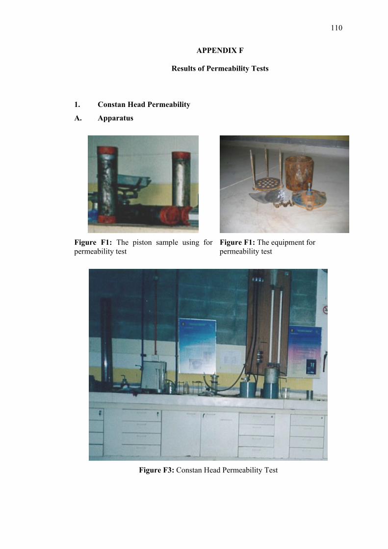
110

APPENDIX F

Results of Permeability Tests

1. Constan Head Permeability

A. Apparatus

Figure F1: The piston sample using for permeability test

Figure F1: The equipment for permeability test

Figure F3: Constan Head Permeability Test

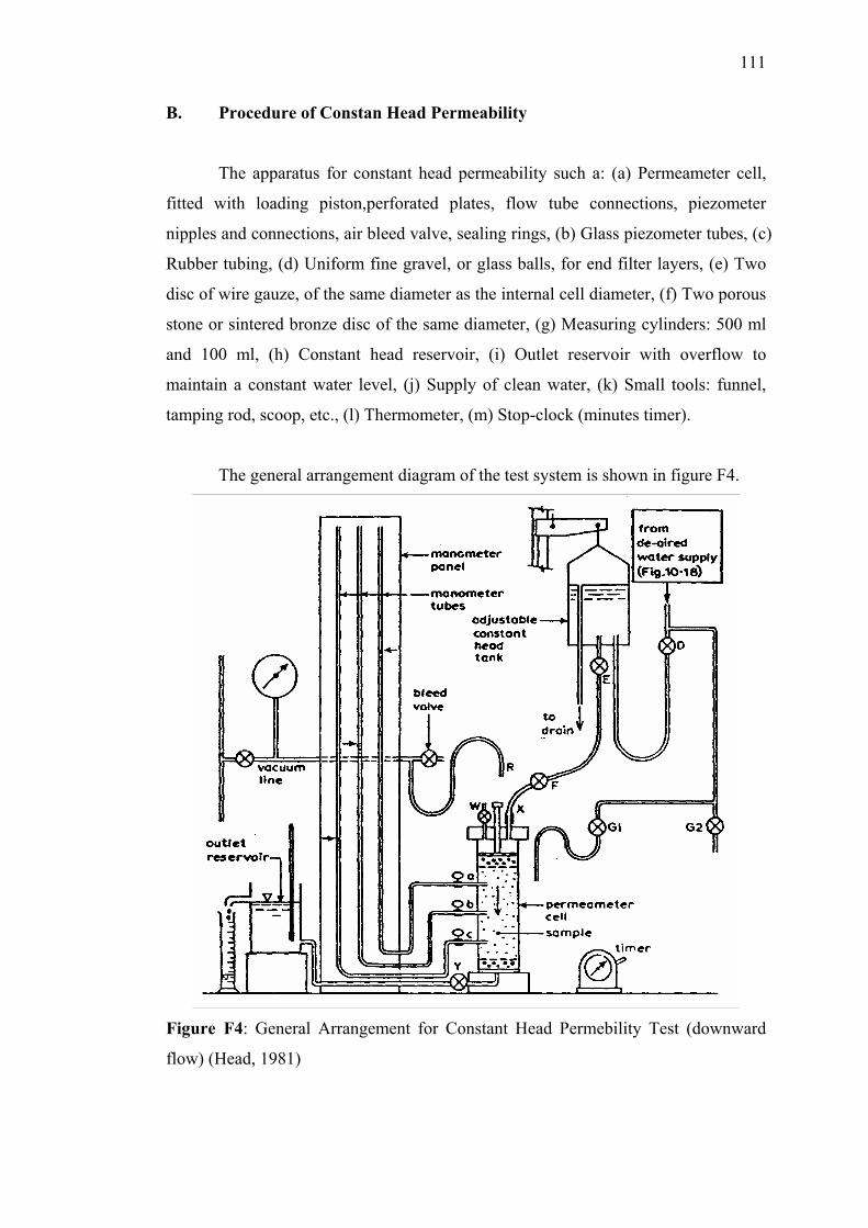
111

B. Procedure of Constan Head Permeability

The apparatus for constant head permeability such a: (a) Permeameter cell,

fitted with loading piston,perforated plates, flow tube connections, piezometer

nipples and connections, air bleed valve, sealing rings, (b) Glass piezometer tubes, (c)

Rubber tubing, (d) Uniform fine gravel, or glass balls, for end filter layers, (e) Two

disc of wire gauze, of the same diameter as the internal cell diameter, (f) Two porous

stone or sintered bronze disc of the same diameter, (g) Measuring cylinders: 500 ml

and 100 ml, (h) Constant head reservoir, (i) Outlet reservoir with overflow to

maintain a constant water level, (j) Supply of clean water, (k) Small tools: funnel,

tamping rod, scoop, etc., (l) Thermometer, (m) Stop-clock (minutes timer).

The general arrangement diagram of the test system is shown in figure F4.

Figure F4: General Arrangement for Constant Head Permebility Test (downward

flow) (Head, 1981)

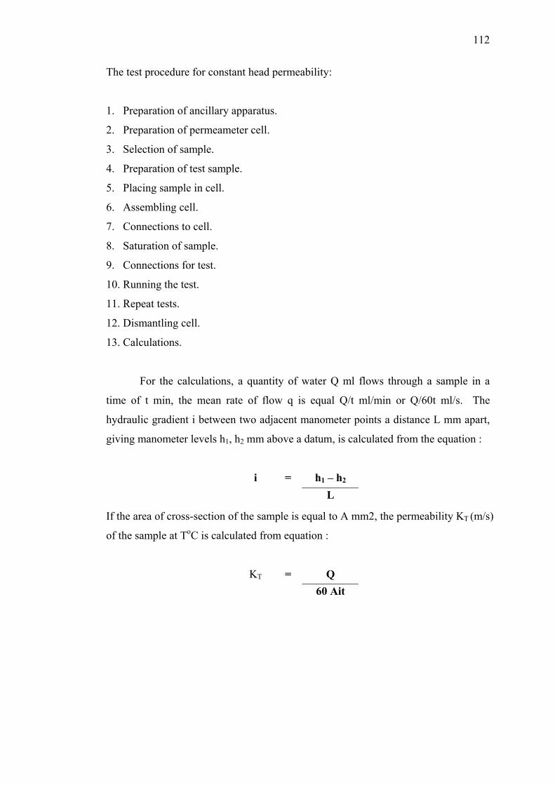
112

The test procedure for constant head permeability:

1. Preparation of ancillary apparatus.

2. Preparation of permeameter cell.

3. Selection of sample.

4. Preparation of test sample.

5. Placing sample in cell.

6. Assembling cell.

7. Connections to cell.

8. Saturation of sample.

9. Connections for test.

10. Running the test.

11. Repeat tests.

12. Dismantling cell.

13. Calculations.

For the calculations, a quantity of water Q ml flows through a sample in a

time of t min, the mean rate of flow q is equal Q/t ml/min or Q/60t ml/s. The

hydraulic gradient i between two adjacent manometer points a distance L mm apart,

giving manometer levels h1, h2 mm above a datum, is calculated from the equation :

i = h1 – h2

L

If the area of cross-section of the sample is equal to A mm2, the permeability KT (m/s)

of the sample at ToC is calculated from equation :

KT = Q

60 Ait

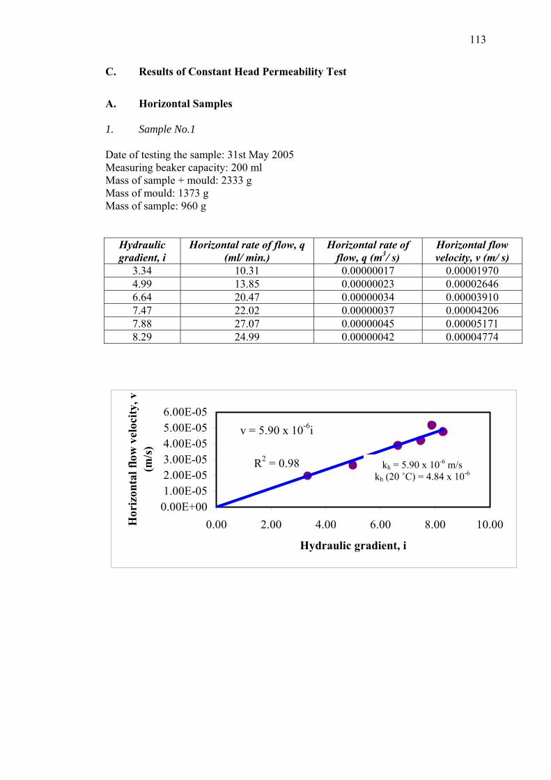
113

C. Results of Constant Head Permeability Test

A. Horizontal Samples 1. Sample No.1 Date of testing the sample: 31st May 2005 Measuring beaker capacity: 200 ml Mass of sample + mould: 2333 g Mass of mould: 1373 g Mass of sample: 960 g

Hydraulic gradient, i

Horizontal rate of flow, q (ml/ min.)

Horizontal rate of flow, q (m3/ s)

Horizontal flow velocity, v (m/ s)

3.34 10.31 0.00000017 0.00001970 4.99 13.85 0.00000023 0.00002646 6.64 20.47 0.00000034 0.00003910 7.47 22.02 0.00000037 0.00004206 7.88 27.07 0.00000045 0.00005171 8.29 24.99 0.00000042 0.00004774

v = 5.90 x 10-6i

R2 = 0.98

0.00E+001.00E-052.00E-053.00E-054.00E-055.00E-056.00E-05

0.00 2.00 4.00 6

Hydraulic grad

Hor

izon

tal f

low

vel

ocity

, v

(m/s

)

k

kh = 5.90 x 10-6 m/s h (20 ˚C) = 4.84 x 10-6

/

.00 8.00 10.00

ient, i

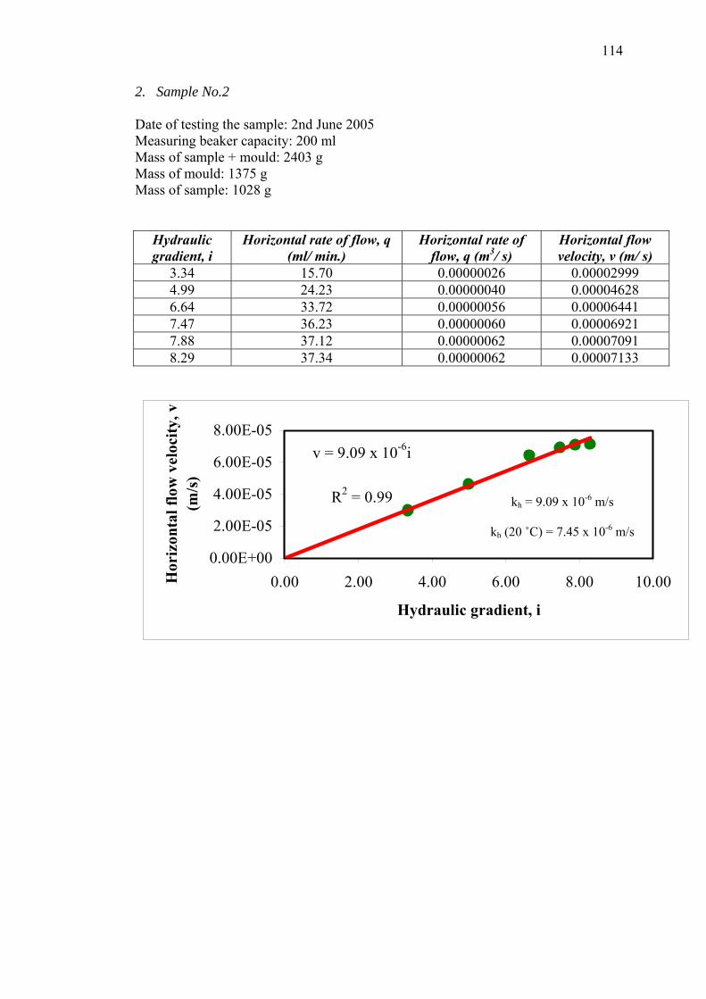
114

2. Sample No.2 Date of testing the sample: 2nd June 2005 Measuring beaker capacity: 200 ml Mass of sample + mould: 2403 g Mass of mould: 1375 g Mass of sample: 1028 g

Hydraulic gradient, i

Horizontal rate of flow, q (ml/ min.)

Horizontal rate of flow, q (m3/ s)

Horizontal flow velocity, v (m/ s)

3.34 15.70 0.00000026 0.00002999 4.99 24.23 0.00000040 0.00004628 6.64 33.72 0.00000056 0.00006441 7.47 36.23 0.00000060 0.00006921 7.88 37.12 0.00000062 0.00007091 8.29 37.34 0.00000062 0.00007133

v = 9.09 x 10-6i

R2 = 0.99

0.00E+00

2.00E-05

4.00E-05

6.00E-05

8.00E-05

0.00 2.00 4.00 6.

Hydraulic grad

Hor

izon

tal f

low

vel

ocity

, v

(m/s

)

kh

kh = 9.09 x 10-6 m/s

(20 ˚C) = 7.45 x 10-6 m/s

00 8.00 10.00

ient, i

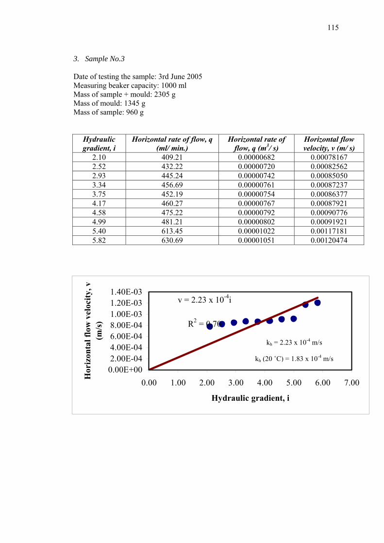
115

3. Sample No.3 Date of testing the sample: 3rd June 2005 Measuring beaker capacity: 1000 ml Mass of sample + mould: 2305 g Mass of mould: 1345 g Mass of sample: 960 g

Hydraulic gradient, i

Horizontal rate of flow, q (ml/ min.)

Horizontal rate of flow, q (m3/ s)

Horizontal flow velocity, v (m/ s)

2.10 409.21 0.00000682 0.00078167 2.52 432.22 0.00000720 0.00082562 2.93 445.24 0.00000742 0.00085050 3.34 456.69 0.00000761 0.00087237 3.75 452.19 0.00000754 0.00086377 4.17 460.27 0.00000767 0.00087921 4.58 475.22 0.00000792 0.00090776 4.99 481.21 0.00000802 0.00091921 5.40 613.45 0.00001022 0.00117181 5.82 630.69 0.00001051 0.00120474

v = 2.23 x 10-4i

R2 = 0.70

0.00E+002.00E-044.00E-046.00E-048.00E-041.00E-031.20E-031.40E-03

0.00 1.00 2.00 3.00 4

Hydraulic gra

Hor

izon

tal f

low

vel

ocity

, v

(m/s

)

kh

kh = 2.23 x 10-4 m/s

(20 ˚C) = 1.83 x 10-4 m/s

.00 5.00 6.00 7.00

dient, i

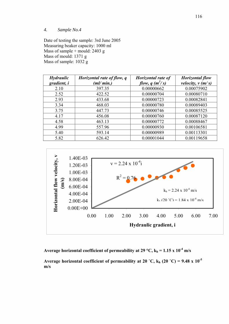
116

4. Sample No.4 Date of testing the sample: 3rd June 2005 Measuring beaker capacity: 1000 ml Mass of sample + mould: 2403 g Mass of mould: 1371 g Mass of sample: 1032 g

Hydraulic gradient, i

Horizontal rate of flow, q (ml/ min.)

Horizontal rate of flow, q (m3/ s)

Horizontal flow velocity, v (m/ s)

2.10 397.35 0.00000662 0.00075902 2.52 422.52 0.00000704 0.00080710 2.93 433.68 0.00000723 0.00082841 3.34 468.03 0.00000780 0.00089403 3.75 447.73 0.00000746 0.00085525 4.17 456.08 0.00000760 0.00087120 4.58 463.13 0.00000772 0.00088467 4.99 557.96 0.00000930 0.00106581 5.40 593.14 0.00000989 0.00113301 5.82 626.42 0.00001044 0.00119658

v = 2.24 x 10-4i

R2 = 0.76

0.00E+002.00E-044.00E-046.00E-048.00E-041.00E-031.20E-031.40E-03

0.00 1.00 2.00 3.00 4.0

Hydraulic grad

Hor

izon

tal f

low

vel

ocity

, v

(m/s

)

kh

Average horizontal coefficient of permeability at 29 °C, kh = Average horizontal coefficient of permeability at 20 ˚C, kh m/s

kh = 2.24 x 10-4 m/s

(20 ˚C) = 1.84 x 10-4 m/s

0 5.00 6.00 7.00

ient, i

1.15 x 10-4 m/s

(20 ˚C) = 9.48 x 10-5

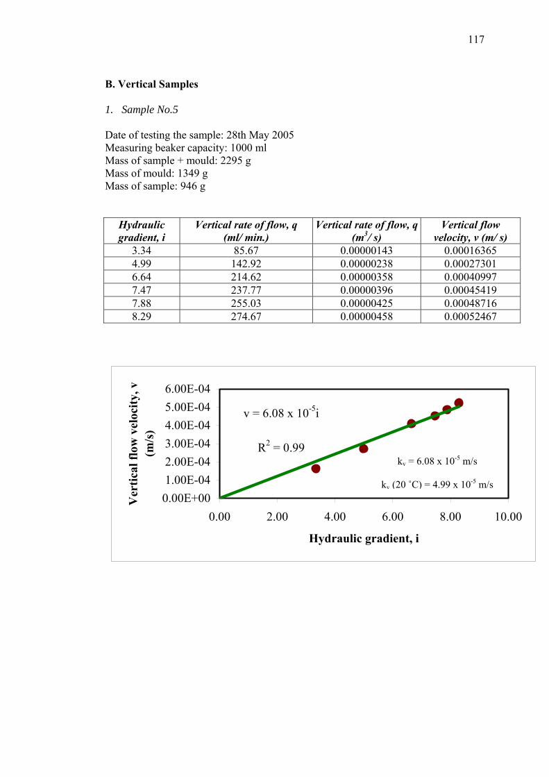
117

B. Vertical Samples 1. Sample No.5 Date of testing the sample: 28th May 2005 Measuring beaker capacity: 1000 ml Mass of sample + mould: 2295 g Mass of mould: 1349 g Mass of sample: 946 g

Hydraulic gradient, i

Vertical rate of flow, q (ml/ min.)

Vertical rate of flow, q (m3/ s)

Vertical flow velocity, v (m/ s)

3.34 85.67 0.00000143 0.00016365 4.99 142.92 0.00000238 0.00027301 6.64 214.62 0.00000358 0.00040997 7.47 237.77 0.00000396 0.00045419 7.88 255.03 0.00000425 0.00048716 8.29 274.67 0.00000458 0.00052467

v = 6.08 x 10-5i

R2 = 0.99

0.00E+001.00E-042.00E-043.00E-044.00E-045.00E-046.00E-04

0.00 2.00 4.00 6.

Hydraulic gradi

Ver

tical

flow

vel

ocity

, v

(m/s

)

kv

kv = 6.08 x 10-5 m/s

(20 ˚C) = 4.99 x 10-5 m/s

00 8.00 10.00

ent, i

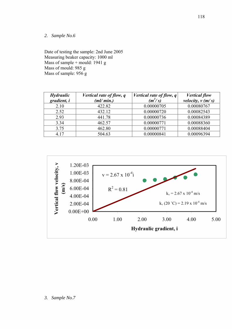
118

2. Sample No.6 Date of testing the sample: 2nd June 2005 Measuring beaker capacity: 1000 ml Mass of sample + mould: 1941 g Mass of mould: 985 g Mass of sample: 956 g

Hydraulic gradient, i

Vertical rate of flow, q (ml/ min.)

Vertical rate of flow, q (m3/ s)

Vertical flow velocity, v (m/ s)

2.10 422.82 0.00000705 0.00080767 2.52 432.12 0.00000720 0.00082543 2.93 441.78 0.00000736 0.00084389 3.34 462.57 0.00000771 0.00088360 3.75 462.80 0.00000771 0.00088404 4.17 504.63 0.00000841 0.00096394

v = 2.67 x 10-4i

R2 = 0.81

0.00E+002.00E-044.00E-046.00E-048.00E-041.00E-031.20E-03

0.00 1.00 2.00 3

Hydraulic grad

Ver

tical

flow

vel

ocity

, v

(m/s

)

kv

3. Sample No.7

kv = 2.67 x 10-4 m/s

(20 ˚C) = 2.19 x 10-4 m/s

.00 4.00 5.00

ient, i

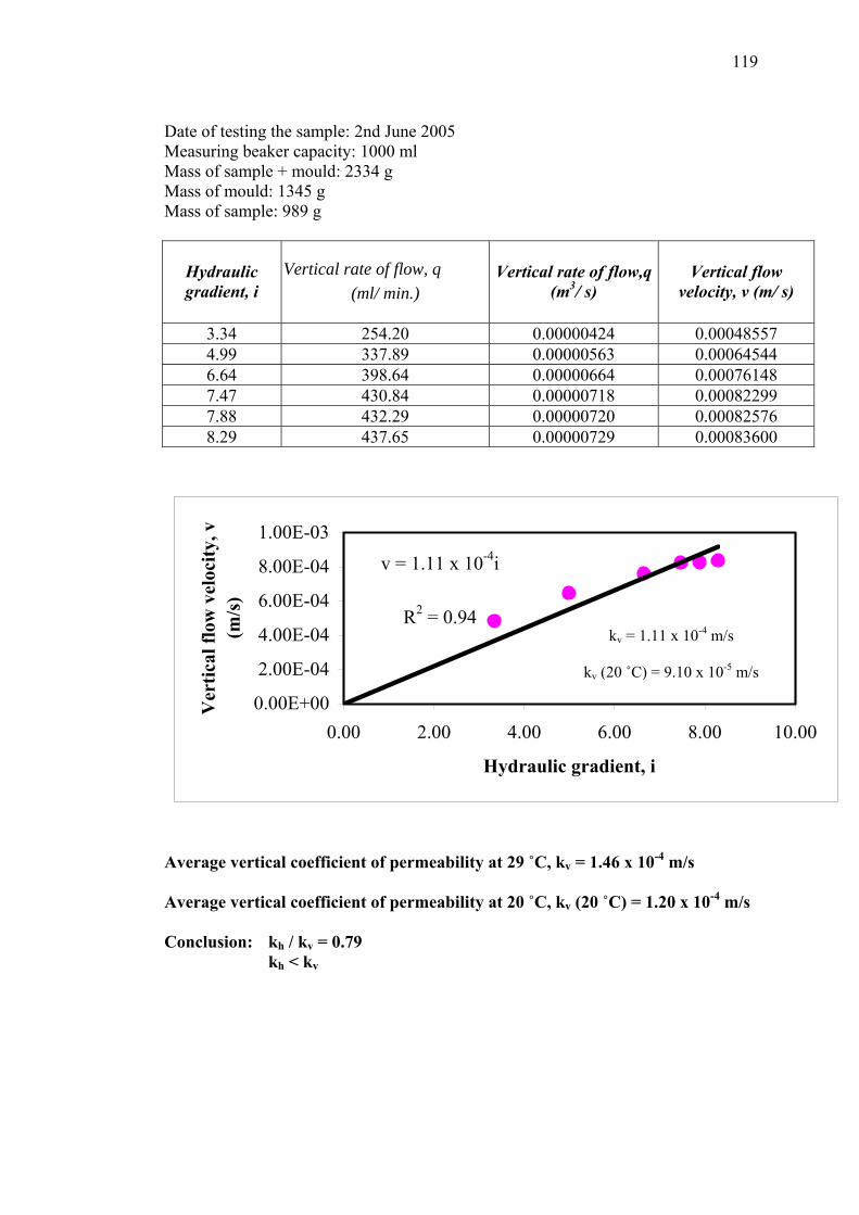
119

Date of testing the sample: 2nd June 2005 Measuring beaker capacity: 1000 ml Mass of sample + mould: 2334 g Mass of mould: 1345 g Mass of sample: 989 g

Hydraulic gradient, i

Vertical rate of flow, q (ml/ min.)

Vertical rate of flow,q

(m3/ s)

Vertical flow

velocity, v (m/ s)

3.34 254.20 0.00000424 0.00048557 4.99 337.89 0.00000563 0.00064544 6.64 398.64 0.00000664 0.00076148 7.47 430.84 0.00000718 0.00082299 7.88 432.29 0.00000720 0.00082576 8.29 437.65 0.00000729 0.00083600

verage vertical coefficient of permeability at 29 ˚C, kv = 1

verage vertical coefficient of permeability at 20 ˚C, kv (20

onclusion: kh / kv = 0.79

v = 1.11 x 10-4i

R2 = 0.94

0.00E+00

2.00E-04

4.00E-04

6.00E-04

8.00E-04

1.00E-03

0.00 2.00 4.00 6

Hydraulic gra

Ver

tical

flow

vel

ocity

, v

(m/s

)

kv

A A C kh < kv

kv = 1.11 x 10-4 m/s

(20 ˚C) = 9.10 x 10-5 m/s

.46 x 10-4 m/s

˚C) = 1.20 x 10-4 m/s

.00 8.00 10.00

dient, i

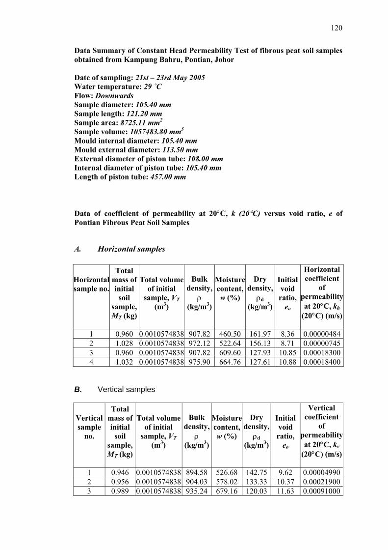
120

Data Summary of Constant Head Permeability Test of fibrous peat soil samples obtained from Kampung Bahru, Pontian, Johor Date of sampling: 21st – 23rd May 2005 Water temperature: 29 ˚C Flow: Downwards Sample diameter: 105.40 mm Sample length: 121.20 mm Sample area: 8725.11 mm2

Sample volume: 1057483.80 mm3

Mould internal diameter: 105.40 mm Mould external diameter: 113.50 mm External diameter of piston tube: 108.00 mm Internal diameter of piston tube: 105.40 mm Length of piston tube: 457.00 mm Data of coefficient of permeability at 20°C, k (20°C) versus void ratio, e of Pontian Fibrous Peat Soil Samples

A. Horizontal samples

Horizontal sample no.

Total mass of initial

soil sample, MT (kg)

Total volume

of initial sample, VT

(m3)

Bulk density,

ρ (kg/m3)

Moisture content, w (%)

Dry

density, ρd

(kg/m3)

Initial void ratio,

eo

Horizontal coefficient

of permeability at 20°C, kh

(20°C) (m/s)

1 0.960 0.0010574838 907.82 460.50 161.97 8.36 0.000004842 1.028 0.0010574838 972.12 522.64 156.13 8.71 0.000007453 0.960 0.0010574838 907.82 609.60 127.93 10.85 0.000183004 1.032 0.0010574838 975.90 664.76 127.61 10.88 0.00018400

B. Vertical samples

Vertical sample

no.

Total mass of initial

soil sample, MT (kg)

Total volume

of initial sample, VT

(m3)

Bulk density,

ρ (kg/m3)

Moisture content, w (%)

Dry

density, ρd

(kg/m3)

Initial void ratio,

eo

Vertical coefficient

of permeability at 20°C, kv

(20°C) (m/s)

1 0.946 0.0010574838 894.58 526.68 142.75 9.62 0.000049902 0.956 0.0010574838 904.03 578.02 133.33 10.37 0.000219003 0.989 0.0010574838 935.24 679.16 120.03 11.63 0.00091000

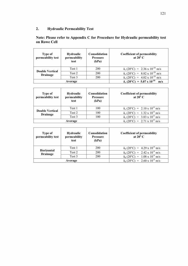
121

2. Hydraulic Permeability Test Note: Please refer to Appendix C for Procedure for Hydraulic permeability test on Rowe Cell

Type of

permeability test

Hydraulic permeability

test

ConsolidationPressure

(kPa)

Coefficient of permeability at 20o C

Test 1 200 kv (20°C) = 2.36 x 10-10 m/s Test 2 200 kv (20°C) = 8.82 x 10-10 m/s

Double Vertical Drainage

Test 3 200 kv (20°C) = 4.02 x 10-10 m/s Average kv (20°C) = 5.07 x 10-10 m/s

Type of permeability test

Hydraulic permeability

test

ConsolidationPressure

(kPa)

Coefficient of permeability at 20o C

Test 1 100 kv (20°C) = 2.10 x 10-9 m/s Test 2 100 kv (20°C) = 1.32 x 10-9 m/s

Double Vertical Drainage

Test 3 100 kv (20°C) = 3.83 x 10-9 m/s Average kv (20°C) = 2.71 x 10-9 m/s

Type of permeability test

Hydraulic permeability

test

ConsolidationPressure

(kPa)

Coefficient of permeability at 20o C

Test 1 200 kh (20°C) = 4.29 x 10-9 m/s Test 2 200 kh (20°C) = 2.42 x 10-9 m/s

Horizontal Drainage

Test 3 200 kh (20°C) = 1.08 x 10-9 m/s Average kh (20°C) = 2.60 x 10-9 m/s

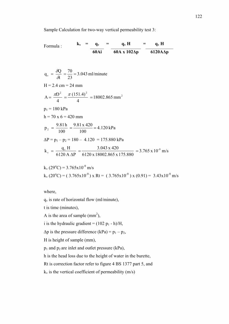
122

Sample Calculation for two-way vertical permeability test 3:

kv = qv = qv H = qv H

60Ai 60A x 102∆p 6120A∆p Formula :

ml/minute 3.043 2370

tQ qv ===

δδ

H = 2.4 cm = 24 mm

222

mm 18002.865 4

(151.4) 4D A ===

ππ

p1 = 180 kPa

h = 70 x 6 = 420 mm

kPa 4.120 100

420 x 9.81 100

h 81.9 p 2 ===

∆P = p1 – p2 = 180 – 4.120 = 175.880 kPa

m/s 10 x 3.765 175.880x 18002.865 x 6120

420 x 3.043 PA 6120

H q k 9-vv ==

∆=

kv (29oC) = 3.765x10-9 m/s

kv (20oC) = ( 3.765x10-9 ) x Rt = ( 3.765x10-9 ) x (0.91) = 3.43x10-9 m/s

where,

qv is rate of horizontal flow (ml/minute),

t is time (minutes),

A is the area of sample (mm2),

i is the hydraulic gradient = (102 p1 - h)/H,

∆p is the pressure difference (kPa) = p1 – p2,

H is height of sample (mm),

p1 and p2 are inlet and outlet pressure (kPa),

h is the head loss due to the height of water in the burette,

Rt is correction factor refer to figure 4 BS 1377 part 5, and

kv is the vertical coefficient of permeability (m/s)