cluster analysis (cont.) pertemuan 12 matakuliah: m0614 / data mining & olap tahun : feb - 2010
TRANSCRIPT


Cluster Analysis (cont.) Pertemuan 12
Matakuliah : M0614 / Data Mining & OLAP Tahun : Feb - 2010
Bina Nusantara
Pada akhir pertemuan ini, diharapkan mahasiswa
akan mampu :• Mahasiswa dapat menggunakan teknik analisis
clustering: Partitioning, hierarchical, dan model-based clustering pada data mining. (C3)
Learning Outcomes
3
Bina Nusantara
Acknowledgments
These slides have been adapted from Han, J., Kamber, M., & Pei, Y. Data Mining: Concepts and Technique and Tan, P.-N., Steinbach, M., & Kumar, V. Introduction to Data Mining.
Bina Nusantara
• A categorization of major clustering methods: Hiararchical methods
• A categorization of major clustering methods: Model-based clustering methods
• Summary
Outline Materi
5
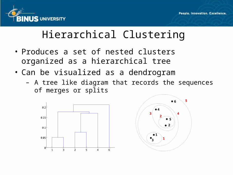
Hierarchical Clustering
• Produces a set of nested clusters organized as a hierarchical tree
• Can be visualized as a dendrogram– A tree like diagram that records the sequences of
merges or splits
1 3 2 5 4 60
0.05
0.1
0.15
0.2
1
2
3
4
5
6
1
23 4
5
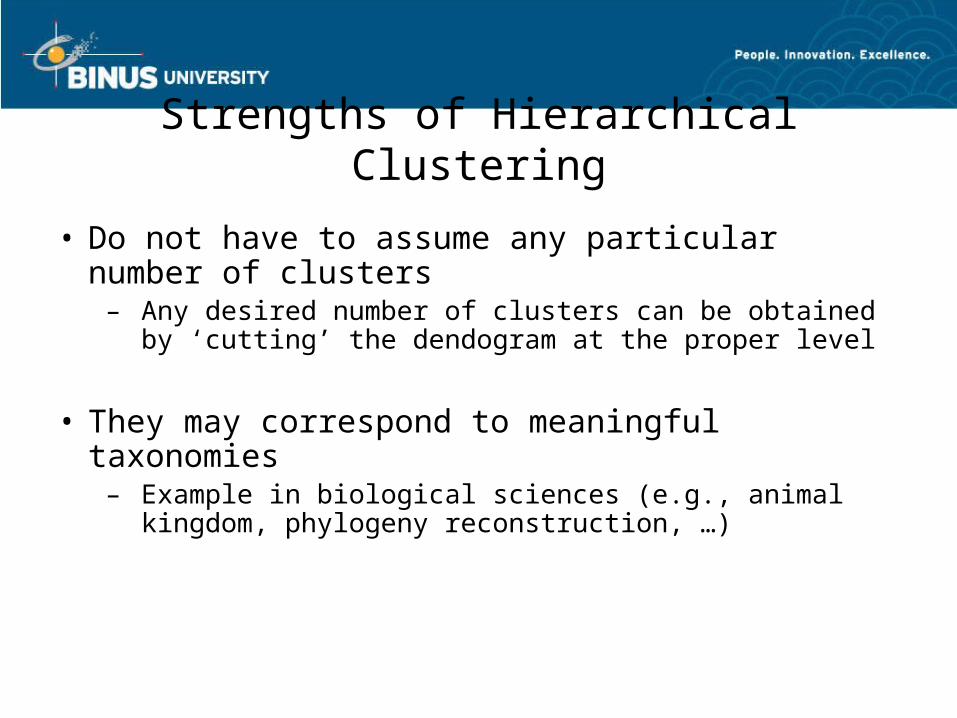
Strengths of Hierarchical Clustering
• Do not have to assume any particular number of clusters
– Any desired number of clusters can be obtained by ‘cutting’ the dendogram at the proper level
• They may correspond to meaningful taxonomies– Example in biological sciences (e.g., animal kingdom,
phylogeny reconstruction, …)
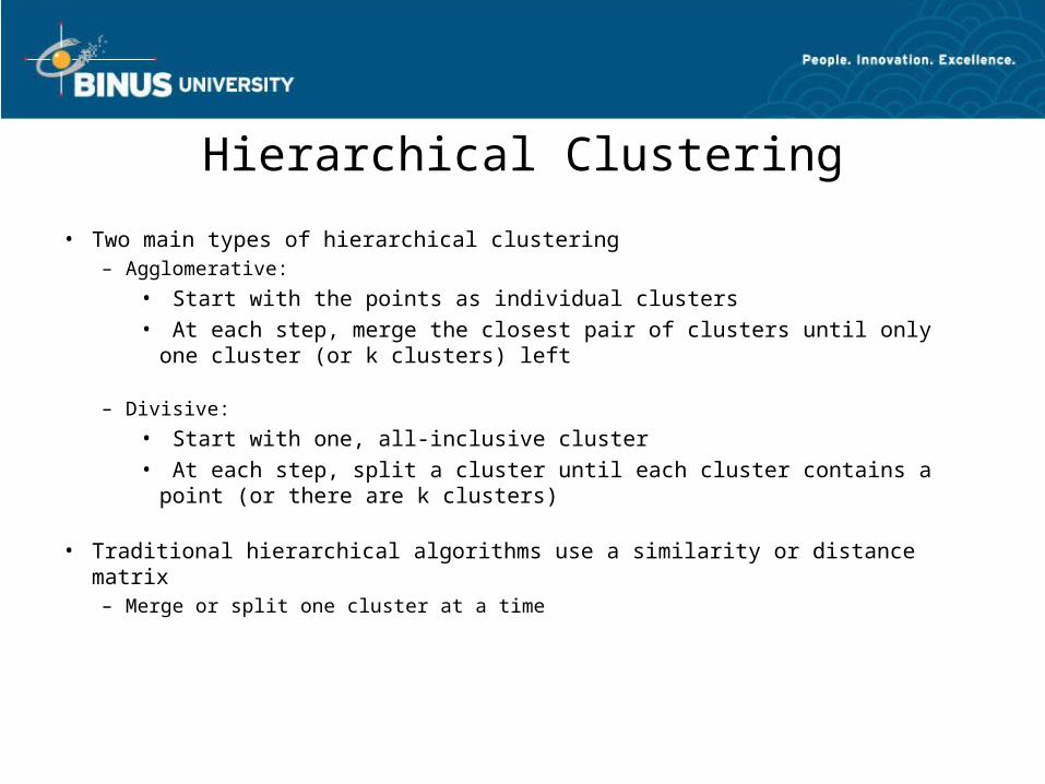
Hierarchical Clustering
• Two main types of hierarchical clustering– Agglomerative:
• Start with the points as individual clusters• At each step, merge the closest pair of clusters until only one
cluster (or k clusters) left
– Divisive:
• Start with one, all-inclusive cluster • At each step, split a cluster until each cluster contains a point (or
there are k clusters)
• Traditional hierarchical algorithms use a similarity or distance matrix– Merge or split one cluster at a time
April 21, 2023Data Mining: Concepts and
Techniques 9
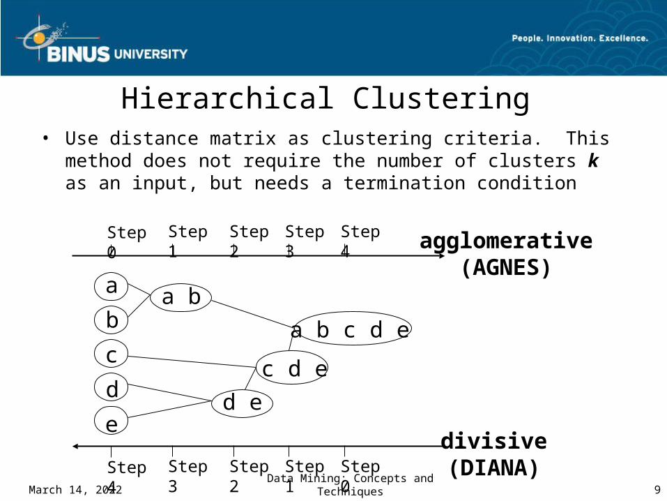
Hierarchical Clustering• Use distance matrix as clustering criteria. This method
does not require the number of clusters k as an input, but needs a termination condition
Step 0 Step 1 Step 2 Step 3 Step 4
b
d
c
e
a a b
d e
c d e
a b c d e
Step 4 Step 3 Step 2 Step 1 Step 0
agglomerative(AGNES)
divisive(DIANA)
April 21, 2023Data Mining: Concepts and
Techniques 10
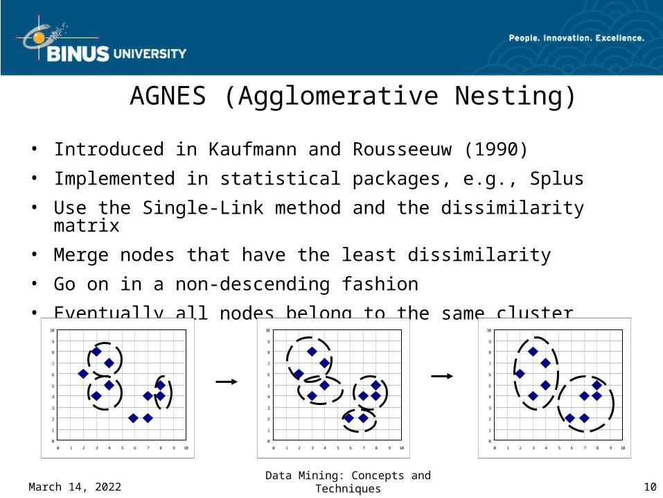
AGNES (Agglomerative Nesting)
• Introduced in Kaufmann and Rousseeuw (1990)
• Implemented in statistical packages, e.g., Splus
• Use the Single-Link method and the dissimilarity matrix
• Merge nodes that have the least dissimilarity
• Go on in a non-descending fashion
• Eventually all nodes belong to the same cluster
0
1
2
3
4
5
6
7
8
9
10
0 1 2 3 4 5 6 7 8 9 10
0
1
2
3
4
5
6
7
8
9
10
0 1 2 3 4 5 6 7 8 9 10
0
1
2
3
4
5
6
7
8
9
10
0 1 2 3 4 5 6 7 8 9 10
Agglomerative Clustering Algorithm
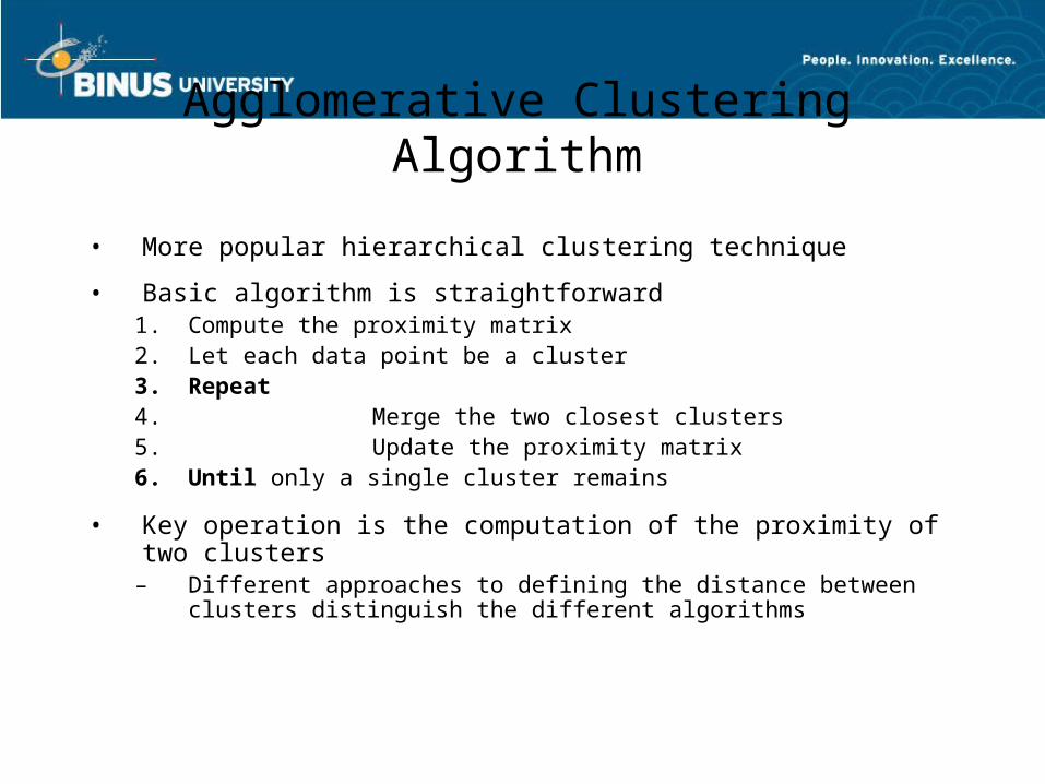
• More popular hierarchical clustering technique
• Basic algorithm is straightforward1. Compute the proximity matrix2. Let each data point be a cluster3. Repeat4. Merge the two closest clusters5. Update the proximity matrix6. Until only a single cluster remains
• Key operation is the computation of the proximity of two clusters
– Different approaches to defining the distance between clusters distinguish the different algorithms
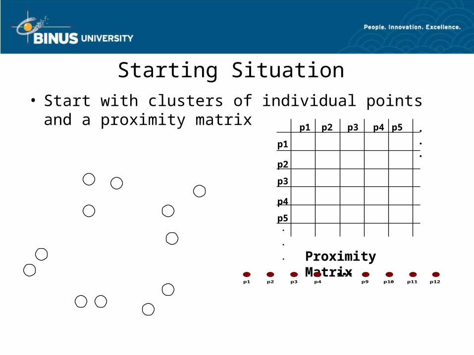
Starting Situation • Start with clusters of individual points and a
proximity matrixp1
p3
p5
p4
p2
p1 p2 p3 p4 p5 . . .
.
.
. Proximity Matrix...
p1 p2 p3 p4 p9 p10 p11 p12
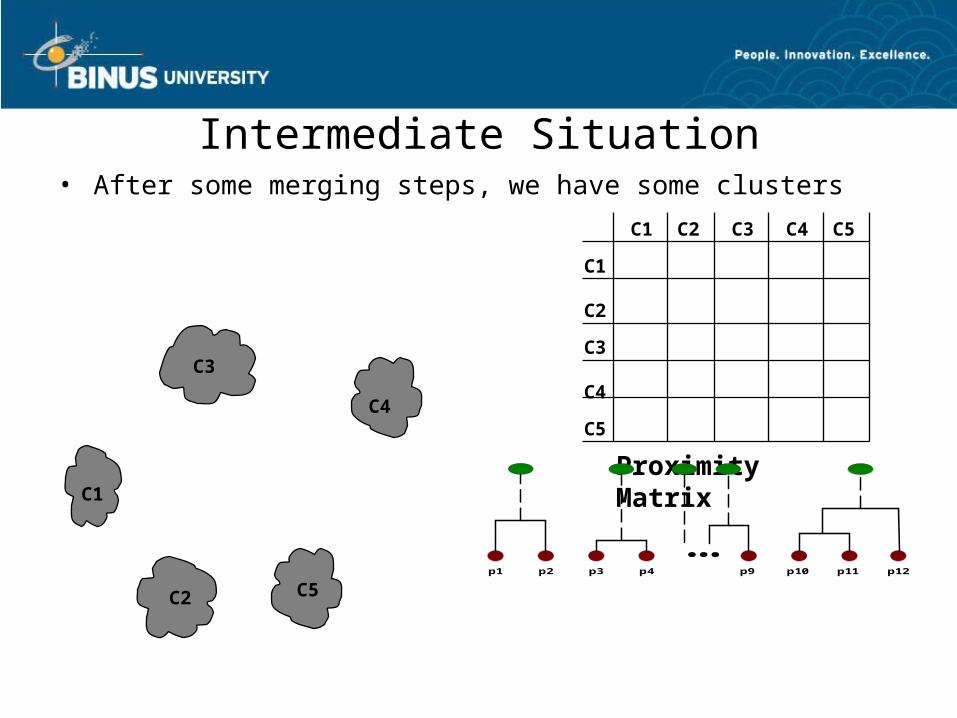
Intermediate Situation• After some merging steps, we have some clusters
C1
C4
C2 C5
C3
C2C1
C1
C3
C5
C4
C2
C3 C4 C5
Proximity Matrix
...p1 p2 p3 p4 p9 p10 p11 p12
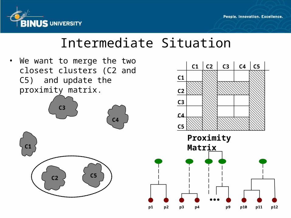
Intermediate Situation• We want to merge the two
closest clusters (C2 and C5) and update the proximity matrix.
C1
C4
C2 C5
C3
C2C1
C1
C3
C5
C4
C2
C3 C4 C5
Proximity Matrix
...p1 p2 p3 p4 p9 p10 p11 p12
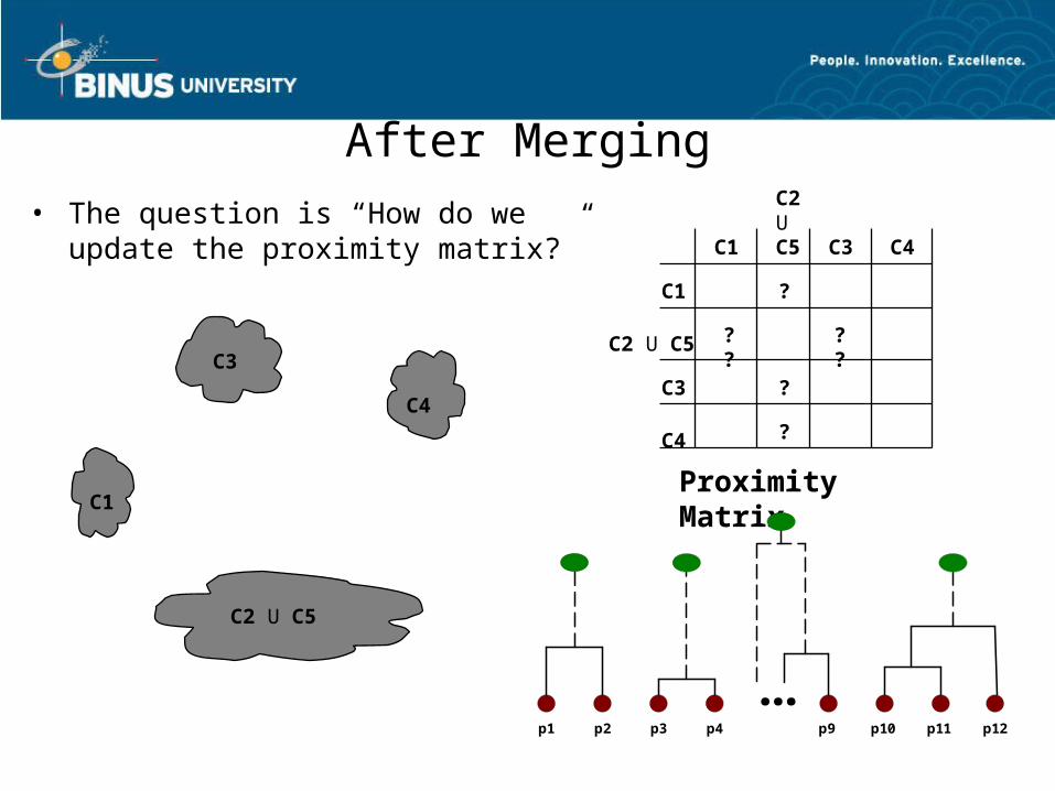
After Merging• The question is “How do we update
the proximity matrix?”
C1
C4
C2 U C5
C3? ? ? ?
?
?
?
C2 U C5C1
C1
C3
C4
C2 U C5
C3 C4
Proximity Matrix
...p1 p2 p3 p4 p9 p10 p11 p12
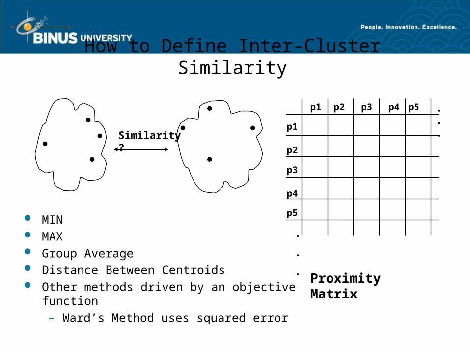
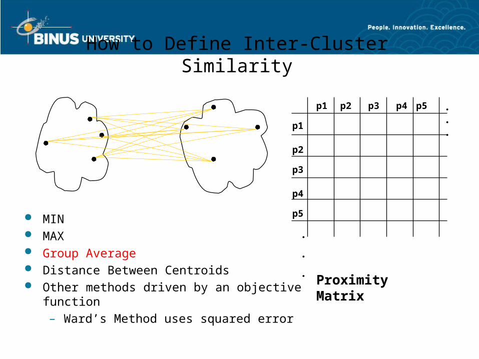
How to Define Inter-Cluster Similarity
p1
p3
p5
p4
p2
p1 p2 p3 p4 p5 . . .
.
.
.
Similarity?
MIN MAX Group Average Distance Between Centroids Other methods driven by an objective function
– Ward’s Method uses squared error
Proximity Matrix
How to Define Inter-Cluster Similarity
p1
p3
p5
p4
p2
p1 p2 p3 p4 p5 . . .
.
.
.Proximity Matrix
MIN MAX Group Average Distance Between Centroids Other methods driven by an objective function
– Ward’s Method uses squared error
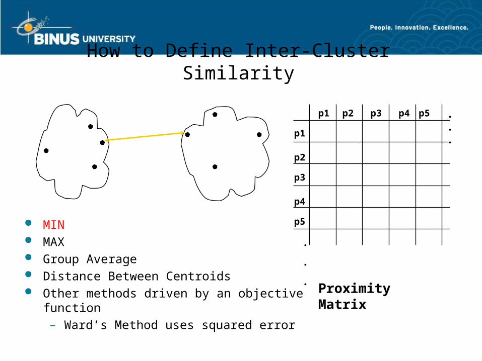
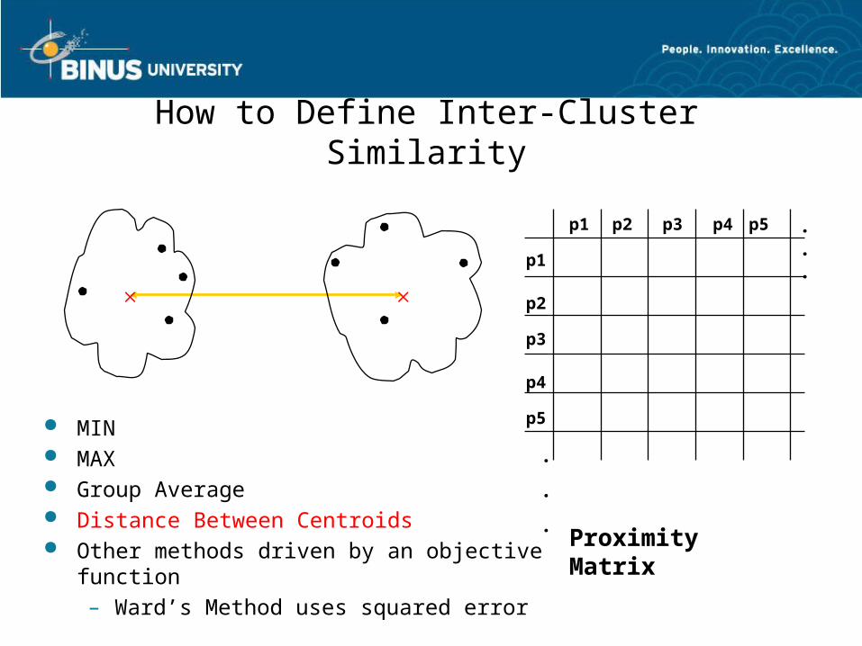
How to Define Inter-Cluster Similarity
p1
p3
p5
p4
p2
p1 p2 p3 p4 p5 . . .
.
.
.Proximity Matrix
MIN MAX Group Average Distance Between Centroids Other methods driven by an objective function
– Ward’s Method uses squared error
How to Define Inter-Cluster Similarity
p1
p3
p5
p4
p2
p1 p2 p3 p4 p5 . . .
.
.
.Proximity Matrix
MIN MAX Group Average Distance Between Centroids Other methods driven by an objective function
– Ward’s Method uses squared error
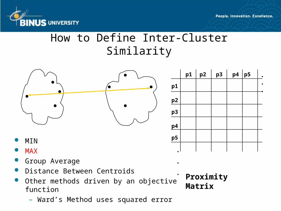
How to Define Inter-Cluster Similarity
p1
p3
p5
p4
p2
p1 p2 p3 p4 p5 . . .
.
.
.Proximity Matrix
MIN MAX Group Average Distance Between Centroids Other methods driven by an objective function
– Ward’s Method uses squared error
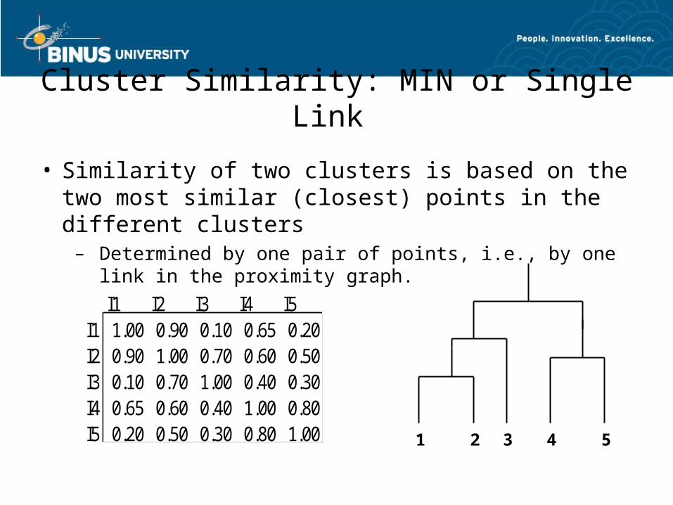
Cluster Similarity: MIN or Single Link
• Similarity of two clusters is based on the two most similar (closest) points in the different clusters
– Determined by one pair of points, i.e., by one link in the proximity graph.
I1 I2 I3 I4 I5I1 1.00 0.90 0.10 0.65 0.20I2 0.90 1.00 0.70 0.60 0.50I3 0.10 0.70 1.00 0.40 0.30I4 0.65 0.60 0.40 1.00 0.80I5 0.20 0.50 0.30 0.80 1.00 1 2 3 4 5
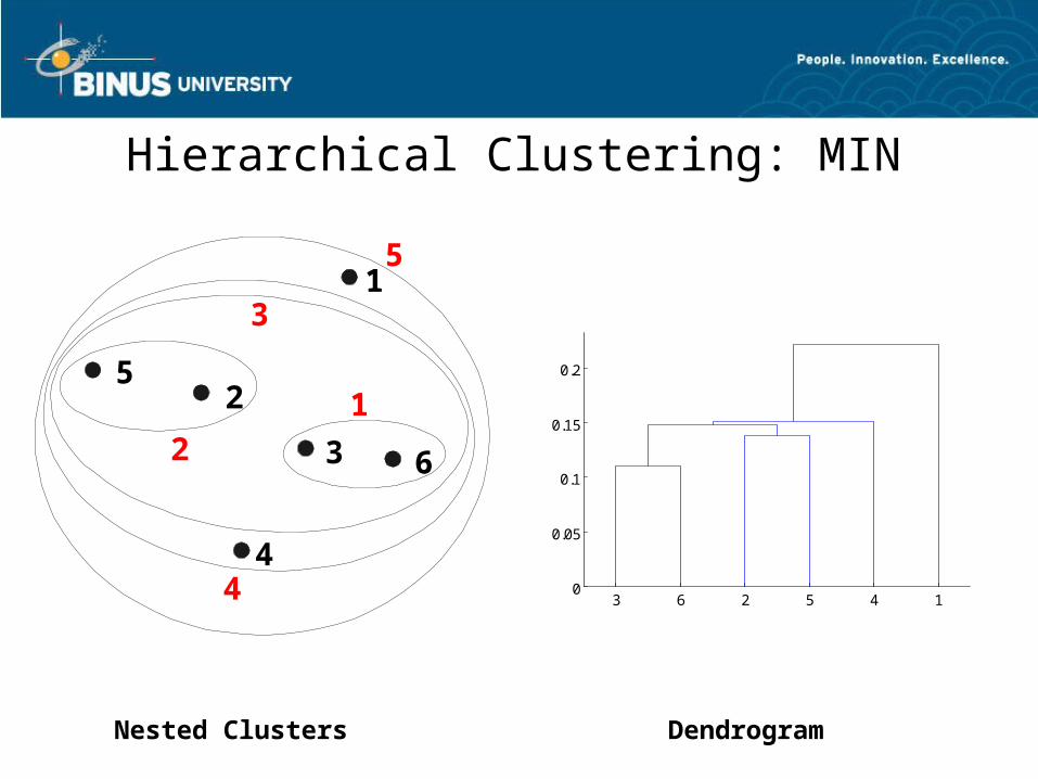
Hierarchical Clustering: MIN
Nested Clusters Dendrogram
1
2
3
4
5
6
1
2
3
4
5
3 6 2 5 4 10
0.05
0.1
0.15
0.2
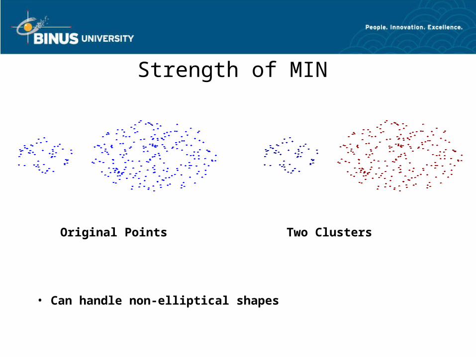
Strength of MIN
Original Points Two Clusters
• Can handle non-elliptical shapes
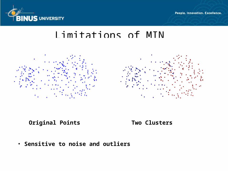
Limitations of MIN
Original Points Two Clusters
• Sensitive to noise and outliers
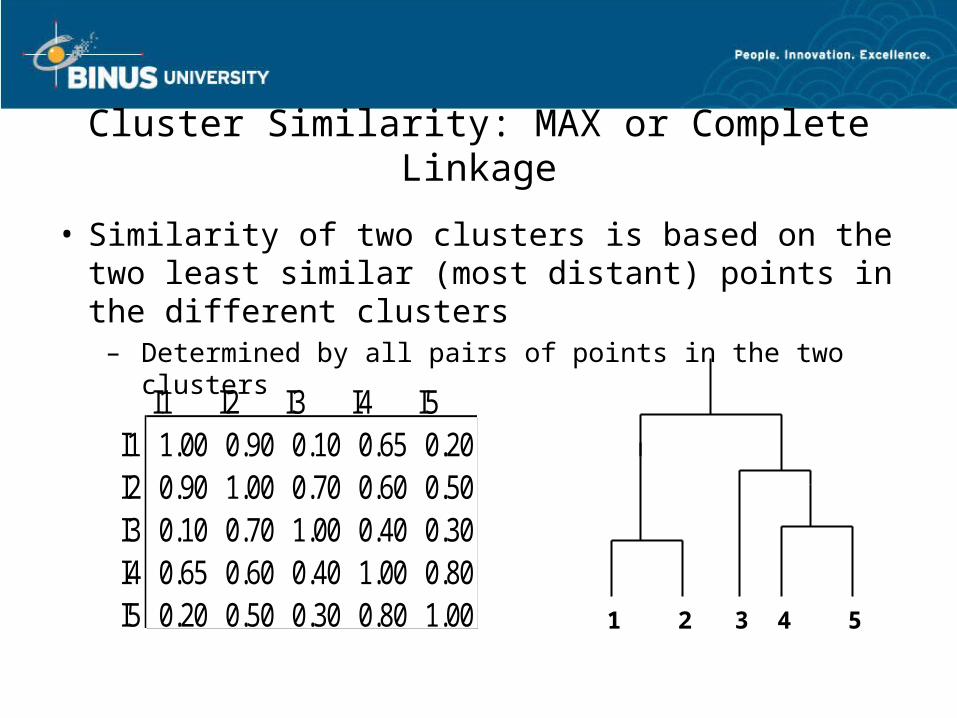
Cluster Similarity: MAX or Complete Linkage
• Similarity of two clusters is based on the two least similar (most distant) points in the different clusters
– Determined by all pairs of points in the two clusters
I1 I2 I3 I4 I5I1 1.00 0.90 0.10 0.65 0.20I2 0.90 1.00 0.70 0.60 0.50I3 0.10 0.70 1.00 0.40 0.30I4 0.65 0.60 0.40 1.00 0.80I5 0.20 0.50 0.30 0.80 1.00 1 2 3 4 5
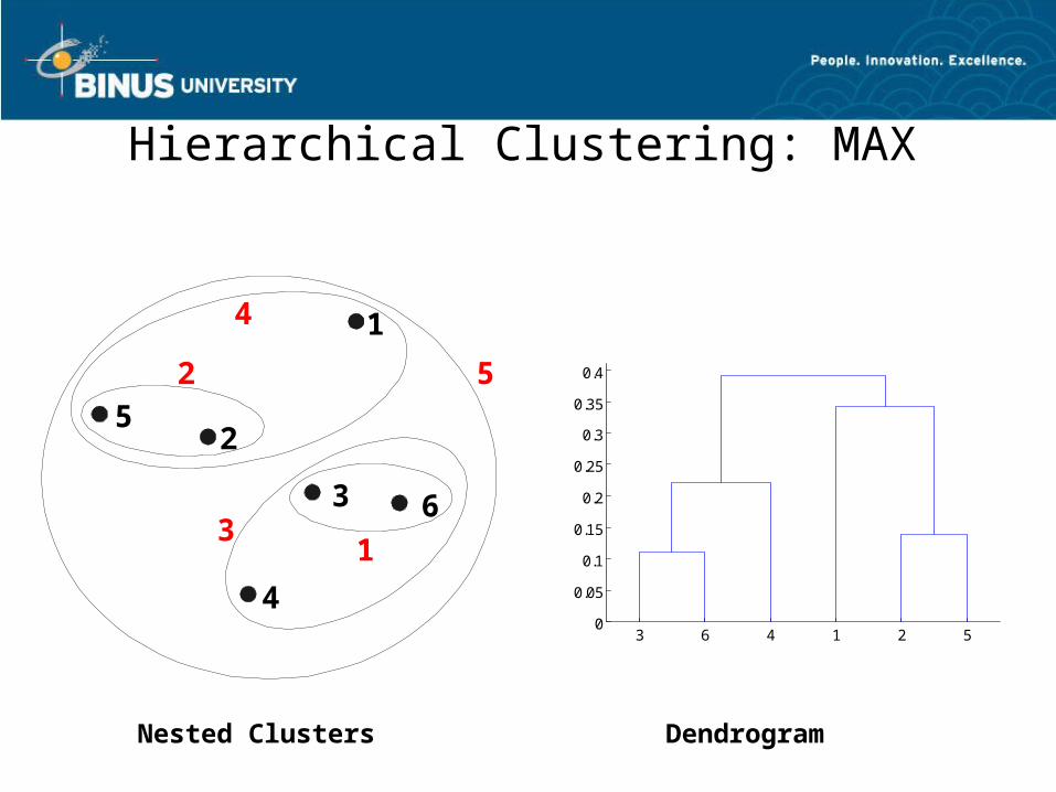
Hierarchical Clustering: MAX
Nested Clusters Dendrogram
3 6 4 1 2 50
0.05
0.1
0.15
0.2
0.25
0.3
0.35
0.4
1
2
3
4
5
6
1
2 5
3
4
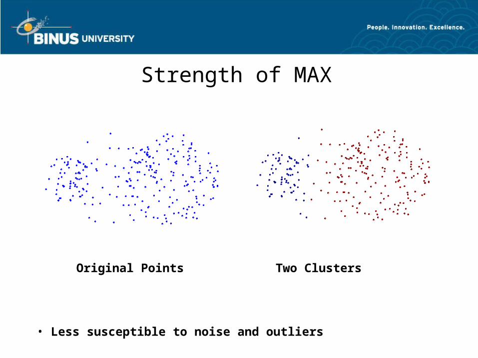
Strength of MAX
Original Points Two Clusters
• Less susceptible to noise and outliers
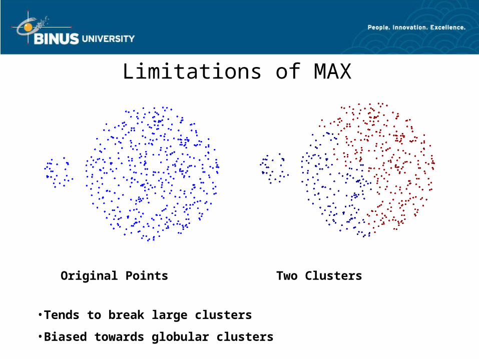
Limitations of MAX
Original Points Two Clusters
•Tends to break large clusters
•Biased towards globular clusters
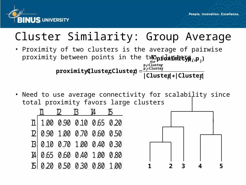
Cluster Similarity: Group Average• Proximity of two clusters is the average of pairwise
proximity between points in the two clusters.
• Need to use average connectivity for scalability since total proximity favors large clusters
||Cluster||Cluster
)p,pproximity(
)Cluster,Clusterproximity(ji
ClusterpClusterp
ji
jijjii
I1 I2 I3 I4 I5I1 1.00 0.90 0.10 0.65 0.20I2 0.90 1.00 0.70 0.60 0.50I3 0.10 0.70 1.00 0.40 0.30I4 0.65 0.60 0.40 1.00 0.80I5 0.20 0.50 0.30 0.80 1.00 1 2 3 4 5
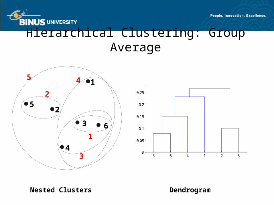
Hierarchical Clustering: Group Average
Nested Clusters Dendrogram
3 6 4 1 2 50
0.05
0.1
0.15
0.2
0.25
1
2
3
4
5
6
1
2
5
3
4
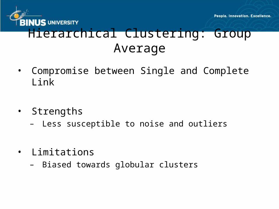
Hierarchical Clustering: Group Average
• Compromise between Single and Complete Link
• Strengths– Less susceptible to noise and outliers
• Limitations– Biased towards globular clusters
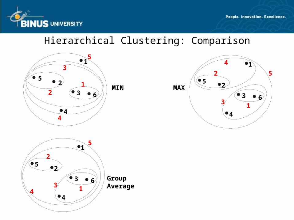
Hierarchical Clustering: Comparison
Group Average
MIN MAX
1
2
3
4
5
61
2
5
34
1
2
3
4
5
61
2 5
3
41
2
3
4
5
6
12
3
4
5
Hierarchical Clustering: Problems and Limitations
• Once a decision is made to combine two clusters, it cannot be undone
• No objective function is directly minimized
• Different schemes have problems with one or more of the following:
– Sensitivity to noise and outliers– Difficulty handling different sized clusters and convex shapes– Breaking large clusters
April 21, 2023Data Mining: Concepts and
Techniques 34
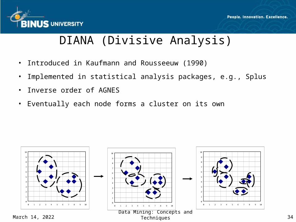
DIANA (Divisive Analysis)
• Introduced in Kaufmann and Rousseeuw (1990)
• Implemented in statistical analysis packages, e.g., Splus
• Inverse order of AGNES
• Eventually each node forms a cluster on its own
0
1
2
3
4
5
6
7
8
9
10
0 1 2 3 4 5 6 7 8 9 100
1
2
3
4
5
6
7
8
9
10
0 1 2 3 4 5 6 7 8 9 10
0
1
2
3
4
5
6
7
8
9
10
0 1 2 3 4 5 6 7 8 9 10
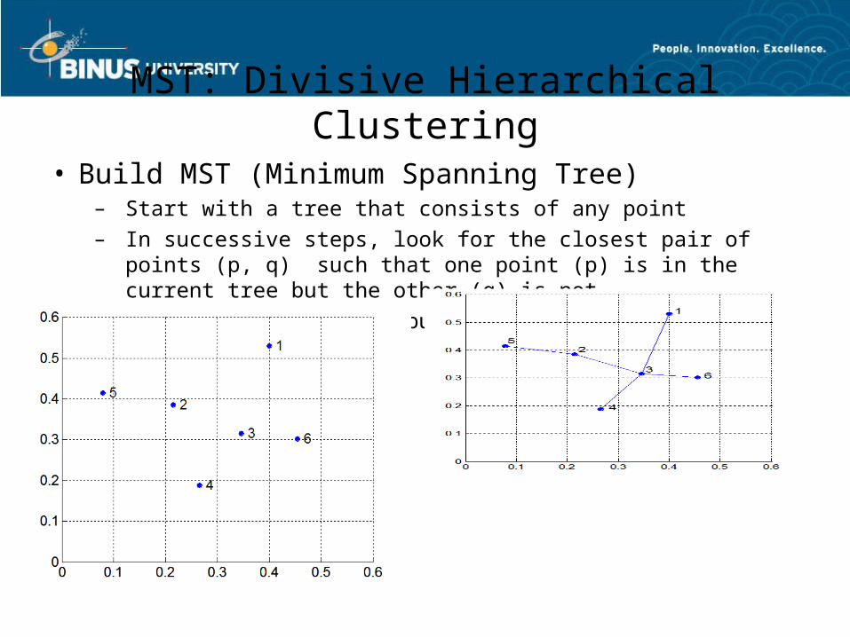
MST: Divisive Hierarchical Clustering• Build MST (Minimum Spanning Tree)
– Start with a tree that consists of any point– In successive steps, look for the closest pair of points (p, q)
such that one point (p) is in the current tree but the other (q) is not
– Add q to the tree and put an edge between p and q
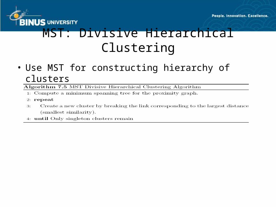
MST: Divisive Hierarchical Clustering
• Use MST for constructing hierarchy of clusters
April 21, 2023Data Mining: Concepts and
Techniques 37
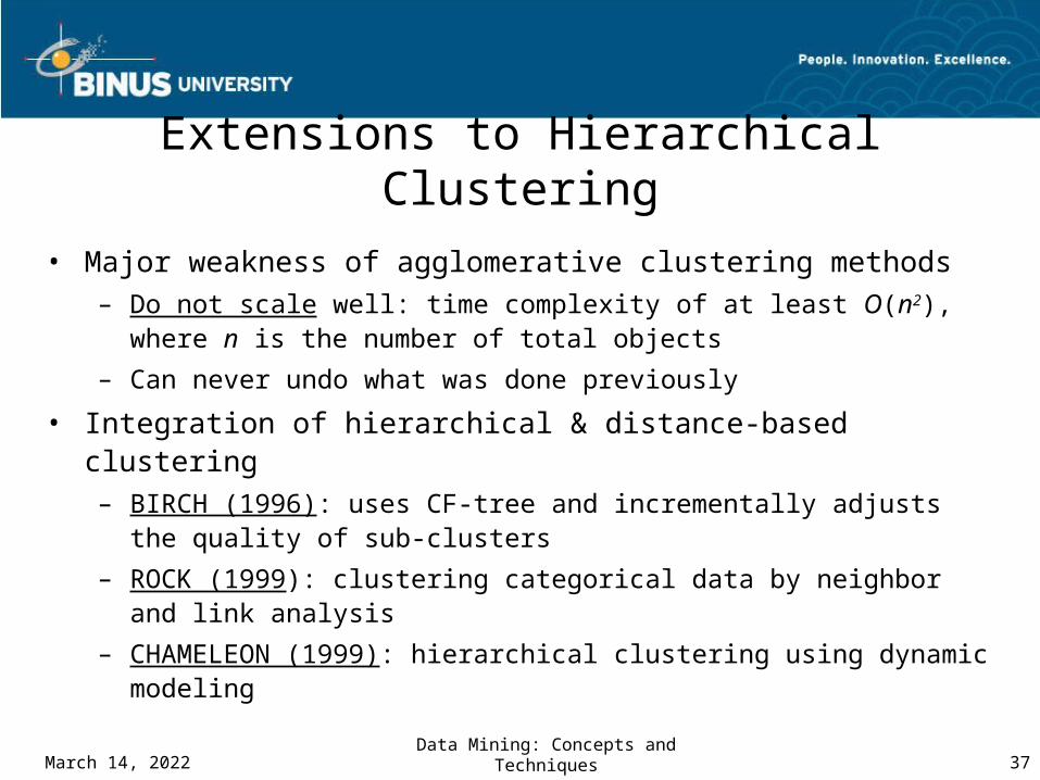
Extensions to Hierarchical Clustering
• Major weakness of agglomerative clustering methods– Do not scale well: time complexity of at least O(n2), where n is
the number of total objects
– Can never undo what was done previously
• Integration of hierarchical & distance-based clustering– BIRCH (1996): uses CF-tree and incrementally adjusts the quality
of sub-clusters
– ROCK (1999): clustering categorical data by neighbor and link analysis
– CHAMELEON (1999): hierarchical clustering using dynamic modeling
April 21, 2023Data Mining: Concepts and
Techniques 38
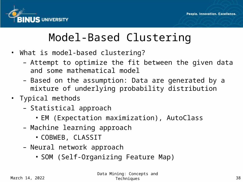
Model-Based Clustering• What is model-based clustering?
– Attempt to optimize the fit between the given data and some mathematical model
– Based on the assumption: Data are generated by a mixture of underlying probability distribution
• Typical methods– Statistical approach
• EM (Expectation maximization), AutoClass– Machine learning approach
• COBWEB, CLASSIT– Neural network approach
• SOM (Self-Organizing Feature Map)
April 21, 2023Data Mining: Concepts and
Techniques 39
EM — Expectation Maximization
• EM — A popular iterative refinement algorithm
• An extension to k-means– Assign each object to a cluster according to a weight (prob. distribution)
– New means are computed based on weighted measures
• General idea– Starts with an initial estimate of the parameter vector
– Iteratively rescores the patterns against the mixture density produced by the parameter vector
– The rescored patterns are used to update the parameter updates
– Patterns belonging to the same cluster, if they are placed by their scores in a particular component
• Algorithm converges fast but may not be in global optima
April 21, 2023Data Mining: Concepts and
Techniques 40
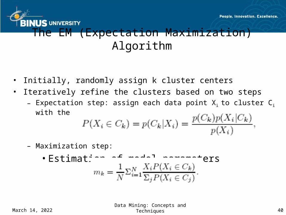
The EM (Expectation Maximization) Algorithm
• Initially, randomly assign k cluster centers• Iteratively refine the clusters based on two steps
– Expectation step: assign each data point Xi to cluster Ci with the following probability
– Maximization step:
• Estimation of model parameters
April 21, 2023Data Mining: Concepts and
Techniques 41
Conceptual Clustering
• Conceptual clustering– A form of clustering in machine learning– Produces a classification scheme for a set of unlabeled objects– Finds characteristic description for each concept (class)
• COBWEB – A popular a simple method of incremental conceptual learning– Creates a hierarchical clustering in the form of a classification tree– Each node refers to a concept and contains a probabilistic
description of that concept
April 21, 2023Data Mining: Concepts and
Techniques 42
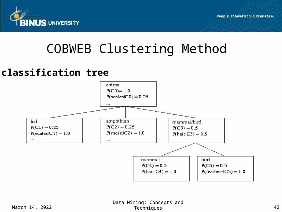
COBWEB Clustering Method
A classification tree
April 21, 2023Data Mining: Concepts and
Techniques 43
More on Conceptual Clustering• Limitations of COBWEB
– The assumption that the attributes are independent of each other is often too strong because correlation may exist
– Not suitable for clustering large database data – skewed tree and expensive probability distributions
• CLASSIT
– an extension of COBWEB for incremental clustering of continuous data
– suffers similar problems as COBWEB
• AutoClass
– Uses Bayesian statistical analysis to estimate the number of clusters
– Popular in industry
April 21, 2023Data Mining: Concepts and
Techniques 44
Neural Network Approach
• Neural network approaches– Represent each cluster as an exemplar, acting as a
“prototype” of the cluster– New objects are distributed to the cluster whose
exemplar is the most similar according to some distance measure
• Typical methods– SOM (Soft-Organizing feature Map)– Competitive learning
• Involves a hierarchical architecture of several units (neurons)
• Neurons compete in a “winner-takes-all” fashion for the object currently being presented
April 21, 2023Data Mining: Concepts and
Techniques 45
Self-Organizing Feature Map (SOM)
• SOMs, also called topological ordered maps, or Kohonen Self-Organizing Feature Map (KSOMs)
• It maps all the points in a high-dimensional source space into a 2 to 3-d target space, s.t., the distance and proximity relationship (i.e., topology) are preserved as much as possible
• Similar to k-means: cluster centers tend to lie in a low-dimensional manifold in the feature space
• Clustering is performed by having several units competing for the current object– The unit whose weight vector is closest to the current object wins
– The winner and its neighbors learn by having their weights adjusted
• SOMs are believed to resemble processing that can occur in the brain
• Useful for visualizing high-dimensional data in 2- or 3-D space
April 21, 2023Data Mining: Concepts and
Techniques 46
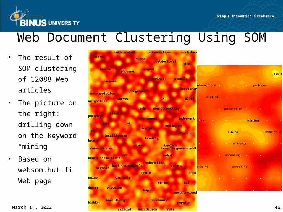
Web Document Clustering Using SOM• The result of
SOM clustering
of 12088 Web
articles
• The picture on
the right:
drilling down on
the keyword
“mining”
• Based on
websom.hut.fi
Web page

April 21, 2023Data Mining: Concepts and
Techniques 47
User-Guided Clustering
name
office
position
Professorcourse-id
name
area
course
semester
instructor
office
position
Studentname
student
course
semester
unit
Register
grade
professor
student
degree
Advise
name
Group
person
group
Work-In
area
year
conf
Publicationtitle
title
Publishauthor
Target of clustering
User hint
CourseOpen-course
• User usually has a goal of clustering, e.g., clustering students by research area
• User specifies his clustering goal to CrossClus
April 21, 2023Data Mining: Concepts and
Techniques 48
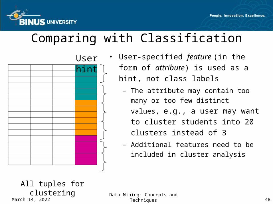
Comparing with Classification• User-specified feature (in the form of
attribute) is used as a hint, not class labels
– The attribute may contain too many
or too few distinct values, e.g., a user may want to cluster students into 20 clusters instead of 3
– Additional features need to be included in cluster analysis
All tuples for clustering
User hint
April 21, 2023Data Mining: Concepts and
Techniques 49
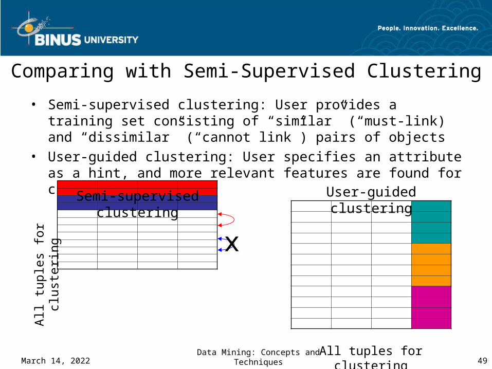
Comparing with Semi-Supervised Clustering
• Semi-supervised clustering: User provides a training set consisting of “similar” (“must-link) and “dissimilar” (“cannot link”) pairs of objects
• User-guided clustering: User specifies an attribute as a hint, and more relevant features are found for clustering
All
tupl
es f
or c
lust
erin
g
Semi-supervised clustering
All tuples for clustering
User-guided clustering
x
April 21, 2023Data Mining: Concepts and
Techniques 50
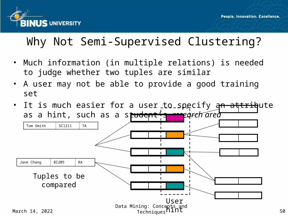
Why Not Semi-Supervised Clustering?
• Much information (in multiple relations) is needed to judge whether two tuples are similar
• A user may not be able to provide a good training set• It is much easier for a user to specify an attribute as a hint,
such as a student’s research area
Tom Smith SC1211 TA
Jane Chang BI205 RA
Tuples to be compared
User hint
April 21, 2023Data Mining: Concepts and
Techniques 51
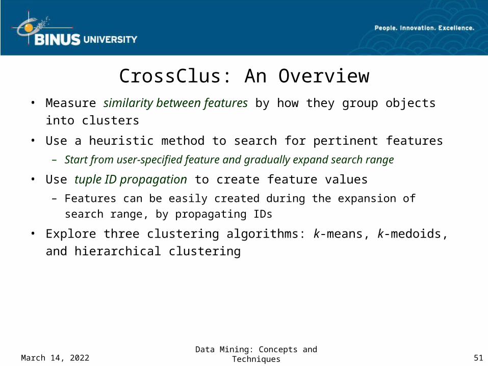
CrossClus: An Overview• Measure similarity between features by how they group objects
into clusters
• Use a heuristic method to search for pertinent features
– Start from user-specified feature and gradually expand search range
• Use tuple ID propagation to create feature values
– Features can be easily created during the expansion of search range, by propagating IDs
• Explore three clustering algorithms: k-means, k-medoids, and hierarchical clustering
April 21, 2023Data Mining: Concepts and
Techniques 52
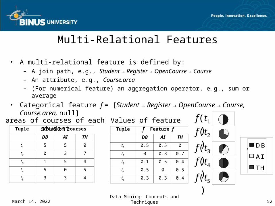
Multi-Relational Features
• A multi-relational feature is defined by: – A join path, e.g., Student → Register → OpenCourse → Course– An attribute, e.g., Course.area– (For numerical feature) an aggregation operator, e.g., sum or average
• Categorical feature f = [Student → Register → OpenCourse → Course, Course.area, null]
Tuple Areas of courses
DB AI TH
t1 5 5 0
t2 0 3 7
t3 1 5 4
t4 5 0 5
t5 3 3 4
areas of courses of each studentTuple Feature f
DB AI TH
t1 0.5 0.5 0
t2 0 0.3 0.7
t3 0.1 0.5 0.4
t4 0.5 0 0.5
t5 0.3 0.3 0.4
Values of feature f f(t1)
f(t2)
f(t3)
f(t4)
f(t5)
DB
AI
TH
April 21, 2023Data Mining: Concepts and
Techniques 53
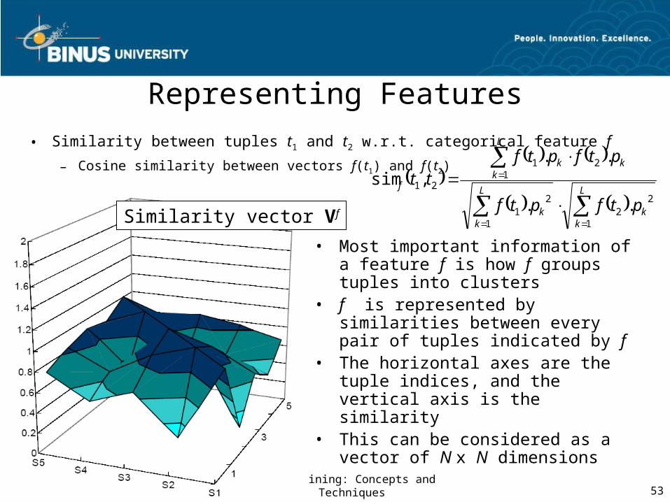
Representing Features
• Similarity between tuples t1 and t2 w.r.t. categorical feature f
– Cosine similarity between vectors f(t1) and f(t2)
• Most important information of a feature f is how f groups tuples into clusters
• f is represented by similarities between every pair of tuples indicated by f
• The horizontal axes are the tuple indices, and the vertical axis is the similarity
• This can be considered as a vector of N x N dimensions
Similarity vector Vf
L
kk
L
kk
L
kkk
f
ptfptf
ptfptftt
1
22
1
21
121
21
..
..,sim
April 21, 2023Data Mining: Concepts and
Techniques 54
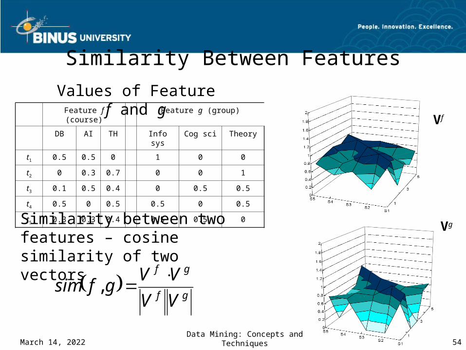
Similarity Between Features
Feature f (course) Feature g (group)
DB AI TH Info sys Cog sci Theory
t1 0.5 0.5 0 1 0 0
t2 0 0.3 0.7 0 0 1
t3 0.1 0.5 0.4 0 0.5 0.5
t4 0.5 0 0.5 0.5 0 0.5
t5 0.3 0.3 0.4 0.5 0.5 0
Values of Feature f and g
Similarity between two features – cosine similarity of two vectors
Vf
Vg
gf
gf
VV
VVgfsim
,
April 21, 2023Data Mining: Concepts and
Techniques 55
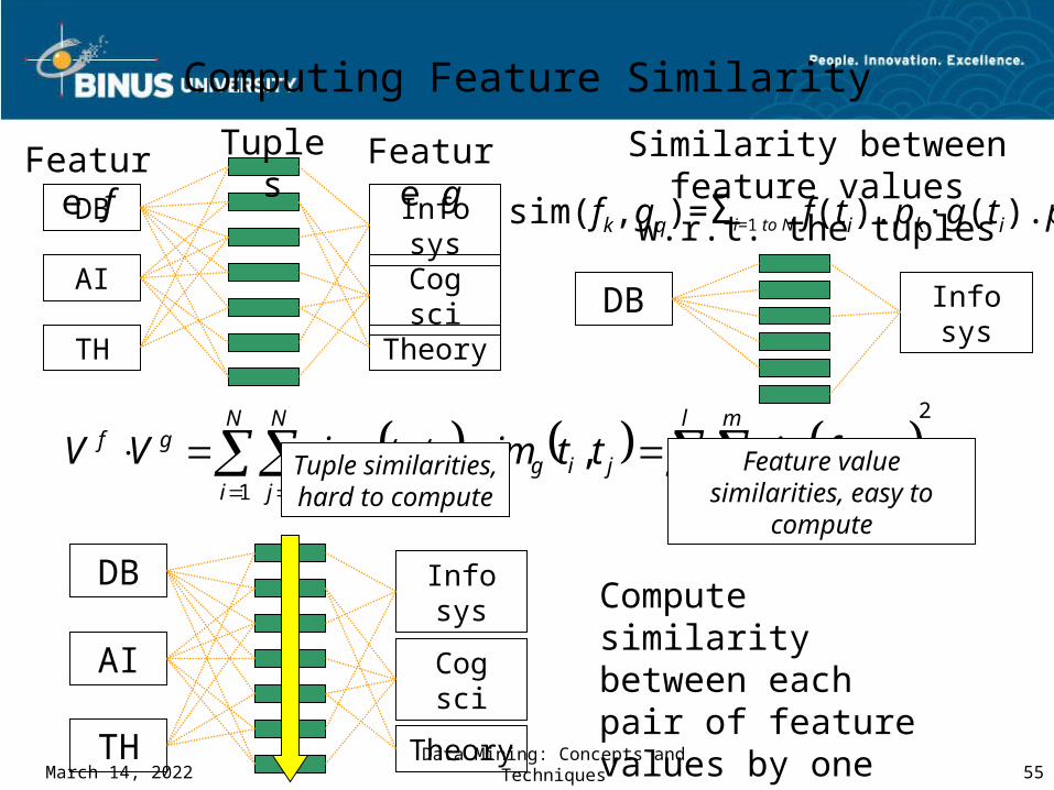
Computing Feature Similarity
TuplesFeature f Feature g
DB
AI
TH
Info sys
Cog sci
Theory
Similarity between feature values w.r.t. the tuples
sim(fk,gq)=Σi=1 to N f(ti).pk∙g(ti).pq
DB Info sys
2
1 11 1
,,,
l
k
m
qqk
N
i
N
jjigjif
gf gfsimttsimttsimVV Tuple similarities, hard to compute
Feature value similarities, easy to compute
DB
AI
TH
Info sys
Cog sci
Theory
Compute similarity between each pair of feature values by one scan on data
April 21, 2023Data Mining: Concepts and
Techniques 56
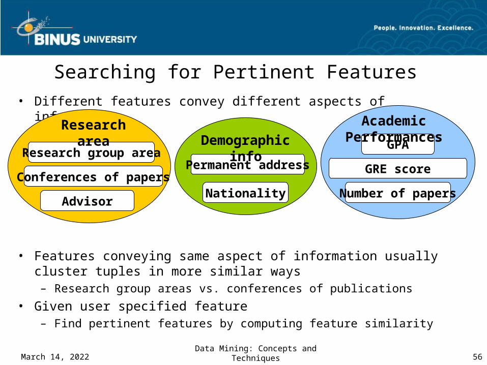
Searching for Pertinent Features• Different features convey different aspects of information
• Features conveying same aspect of information usually cluster tuples in more similar ways– Research group areas vs. conferences of publications
• Given user specified feature– Find pertinent features by computing feature similarity
Research group area
Advisor
Conferences of papers
Research area
GPA
Number of papers
GRE score
Academic Performances
Nationality
Permanent address
Demographic info
April 21, 2023Data Mining: Concepts and
Techniques 57
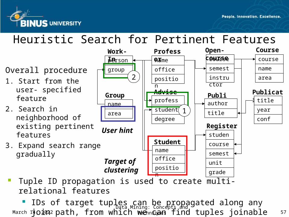
Heuristic Search for Pertinent Features
Overall procedure1. Start from the user-
specified feature2. Search in neighborhood
of existing pertinent features
3. Expand search range gradually
name
office
position
Professor
office
position
Studentname
student
course
semester
unit
Register
grade
professor
student
degree
Advise
person
group
Work-In
name
Group
areayear
conf
Publicationtitle
title
Publishauthor
Target of clustering
User hint
course-id
name
area
Coursecourse
semester
instructor
Open-course
1
2
Tuple ID propagation is used to create multi-relational features IDs of target tuples can be propagated along any join path, from
which we can find tuples joinable with each target tuple
April 21, 2023Data Mining: Concepts and
Techniques 58
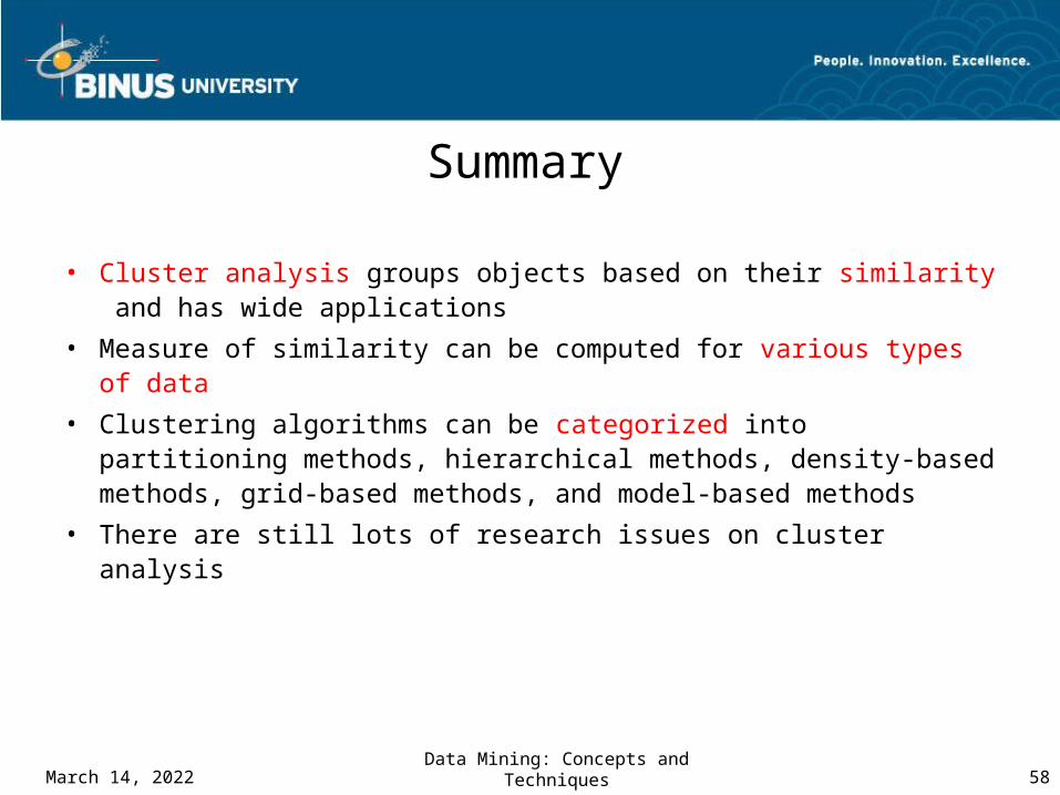
Summary
• Cluster analysis groups objects based on their similarity and has wide applications
• Measure of similarity can be computed for various types of data
• Clustering algorithms can be categorized into partitioning methods, hierarchical methods, density-based methods, grid-based methods, and model-based methods
• There are still lots of research issues on cluster analysis
Bina Nusantara
Dilanjutkan ke pert. 13Applications and Trends in Data Mining